Deep Dive Into Visual Representation and Interrater Agreement Using Data From a High-School Diving Competition

Abstract

In several sporting events, the winner is chosen on the basis of a subjective score. These sports include gymnastics, ice skating, and diving. Unlike for other subjectively judged sports, diving competitions consist of multiple rounds in quick succession on the same apparatus. These multiple rounds lead to an extra layer of complexity in the data, and allow the introduction of graphical constructs and interrater-agreement methods to statistics students. The data are sufficiently easy to understand for students in introductory statistics courses, yet sufficiently complex for upper level students. In this article, I present data from a high-school diving competition that allows for investigation in graphical methods, data manipulation, and interrater agreement methods. I also provide a list of questions for exploration at the end of the document to suggest how an instructor can effectively use the data with students. These questions are not meant to be exhaustive, but rather generative of ideas for an instructor using the data in a classroom setting. Supplementary materials for this article are available online.

Keywords:

• Data visualization
• Intermediate statistics
• Interrater agreement
• Introductory statistics
• Pedagogy
• Statistics in sports

1 Introduction

These data were collected from a regional high school diving competition, originally gathered because the author has a child that has been in competitive diving for almost 10 years. The main reason for collecting the data was to determine whether it is better, in terms of placement in the competition, to do easier dives well or to do more difficult dives less well. Obviously, the best scores will go to those divers who do both easy and difficult dives and do them well. However, if an athlete wants to gain an edge in the competition, should that diver concentrate on doing excellent easy dives or doing less excellent difficult dives?

Every dive performed in competition has an associated “degree of difficulty” (DD) that is determined by the Fédération Internationale de Natation (FINA) (Franklin 2017). Each dive has several elements that make it more or less difficult to perform. Some of the elements include

• number of somersaults (usually 2 or fewer at the high school level);

• position in which the dive is performed (tuck, pike, straight, or free);

• number of twists performed (usually no more than two in high school);

• approach of the dive (forward, back, reverse, or inward);

• height from which the dive is performed (1 m at the high school level);

• type of entry (natural vs. unnatural).

FINA has established a set of formulas and tables that assign DD to each dive based on these elements (Franklin 2017). These data can be used for exercises in introductory statistics courses for students who are learning statistical analysis. Specific exercises are suggested throughout the article.

1.1 The Data

The data were gathered by hand by the author during a high-school regional diving competition. Each of five judges entered a score for each diver and each dive into an electronic system, and those scores were then published onto a large electronic board that all spectators could easily see. As the data were published, the investigator documented each diver’s name, school affiliation, gender, grade, name of dive, position of dive, DD, and scores for each judge on paper scoresheets, which the investigator later transposed into an Excel spreadsheet. The investigator did not obtain information on the affiliation of the judges; therefore, judge bias with regard to school affiliation is not questioned.

In the competition, 13 girls and 12 boys competed. The top three boys and top three girls qualified for the state diving competition. Each judge assigned a score to each dive on a scale of 0 (failed dive) to 10 (perfect dive), in increments of 0.5. In reality, most of the dives were scored between 2.0 and 7.0. Divers performed one dive from the 1-m board in each of 11 rounds, which translates into an average wait time of 15 min between each dive. For each round, the round score was computed by totaling the middle three scores (the maximum and minimum rating are dropped) and multiplying the total by the DD for that dive (Franklin 2018). The final score was the total of the 11 round scores. In the case of a failed dive, the judges were required to agree that the diver did not complete the dive, and all judges assigned a failed dive a score of 0.

Competitive diving at the high-school level requires that a diver complete 11 dives. Five dives are prescribed dives, one from each category of forward, backward, inward, reverse, and twist; another five dives must be from each category, but the diver chooses the dives performed. The eleventh dive is the diver’s choice from any category (Franklin 2018). The dives can be performed in any order, and divers and their coaches can apply several strategies for ordering dives to improve the diver’s overall score. In this particular competition, the easiest dive performed by any diver was a forward dive in a tuck position (DD = 1.2) and the hardest was an inward dive with two-and-one-half somersaults in the tuck position (DD = 2.8). All dives were performed from the 1 m springboard.

The data are given in the file DivingData2018.xlsx, in the supplementary materials, which also includes R Code for data manipulation, visual representation, calculation, regression, and interrater agreement. R packages employed in this article include tidyverse (Wickham 2017), irr (Gamer et al. 2012), and ggplot2 (Wickham 2016), along with their dependencies. The data given in the supplementary materials do not contain divers’ names, grades, and school affiliations, as these variables could easily lead to identification of the diver. Because the data collection involved only observation of public behavior without participation by the investigator in the activities being observed, it is exempt from IRB approval under 45 CFR 46.101(b)(2).

1.2 Questions for Analysis

Originally, the data were collected to answer a question about preferences for easy or difficult dives in terms of final score. Other questions that the diving dataset can illuminate are included below. After each question, the section in which it is discussed is noted.

• In terms of the final score, is it better to perform easier dives well and perform more difficult dives less well, or vice versa? (Section 4)

• To what extent do judges agree on scores for boys? Is the extent the same for girls? (Section 6)

• Which judges, if any, are more lenient than the others? (Section 6)

• How does the DD affect the final score? Is the effect different for boys and girls? (Sections 4 and 5)

• What is the effect of rounding error in score calculation on the final ranking of the divers? (Section 5)

Other questions can direct the exploration of these data, and students can apply many other methods. Other questions relating to these data are listed in the appendix.

Before calculating descriptive statistics and creating visuals, instructors and students need to discuss the nature of the data. Basic discussions—such as whether the data constitute a sample or a population—can help students to understand the concepts of sample and population. In addition, the instructor can ask students to list the variables and the level of measurement for each variable.

Sample Versus Population: The diving data could be viewed as both a sample and as a population. Although they were not collected at random, one could argue that the divers in this sample are representative of all high school divers, at least in the state in which the data were gathered. As such, students could argue that the data are a sample, and they can make inferences from these data about all high-school divers in the state. One could also think of these divers as the population of all divers at the regional contest. In such a case, inferences about these data do not make sense; instead, one can explore the data for relationships using descriptive statistics and visual representation of the data, but hypothesis tests and confidence intervals are irrelevant because an inference about the population is unnecessary when the data reflect the entire population. If students decide that these data are a population, they may also better understand that populations do not need to be large.

Levels of Measurement: Students in introductory courses are often confused by the distinction between levels of measurement (Velleman and Wilkinson 1993). In this dataset, although the judges’ scores can be decimal values, the scores’ range is finite with distinct gaps between possible scores (Lane 2018). The range is 0–10, and the scores occur in increments of 0.5 along that range. Therefore, the scores are discrete. Furthermore, the difference of dive quality between a 5.0 and a 5.5 is not necessarily the same as the difference in quality between a 5.5 and a 6.0. Whereas a score of 5.5 is better than a 5.0, the “quality” of the difference of 0.5 is unclear, and may have different meanings for different judges. Therefore, students must think of the judges’ scores as ordinal measurements. Because the scores are ordinal, summary measures based on percentiles and quartiles are the best measures to describe these data. For most data and situations, simulation studies show that the distinction between ordinal and interval variables is not critical; however, the distinction between categorical and ordinal is important, and missing this distinction can lead to nonsensical results (Baker, Hardyck, and Petrinivic 1966). The level of measurement will be important when examining interrater agreement in Section 6. Table 1 gives details for each variable, including the level of measurement.

Table 1 Table of variables in the diving dataset.

Variable name	Description	Level of measurement	Range
Meet score	Official final score for each diver after 11 dives	Interval	174.7–467.1
Place	Final rank in the competition	Ordinal	1–13 for girls, 1–12 for boys
Gender	Gender of the diver	Categorical	Male or female
Order	Diving order for the competition	Categorical	1–13 for girls, 1–12 for boys
Seed	Placement of diver prior to competition	Ordinal	1–13 for girls, 1–12 for boys
Round	Round of the competition	Categorical	1–11
Dive	FINA number indicating the dive performed	Categorical	103–5223
Position	Position of the diver’s body in the dive	Categorical	Tuck, pike, straight, or free
Approach	Direction of the dive	Categorical	Forward, backward, reverse, inward, twist
DD	FINA degree of difficulty (DD) of the dive	Ordinal	1.2–2.8
Judge 1	Scores from Judge 1	Ordinal	0–10
Judge 2	Scores from Judge 2	Ordinal	0–10
Judge 3	Scores from Judge 3	Ordinal	0–10
Judge 4	Scores from Judge 4	Ordinal	0–10
Judge 5	Scores from Judge 5	Ordinal	0–10
Round score	Score for each diver in each round	Interval	0.0–52.00
Running total	Cumulative score in each round	Interval	13.6–468.4

The “Round Score” for each diver was calculated using the following R Code (also given in DivingDataRCode.txt,) dropping the minimum and maximum judge ratings and totaling the remaining ratings (as described in Franklin (2018)). The code makes use of some syntax specific to tidyverse, such as the “pipe” operator (% >%) for placing the output of one function into another function, and the verb mutate, which allows the user to compute a new variable from a combination of existing variables. The code calculates three new columns in the dataset. The first is the MeanScore, which is the mean of judges’ scores for each round once the maximum and minimum scores have been dropped. The second is a RoundScore, which is the MeanScore times 3 times the DD for each round. The third column is called CumScore. It is the cumulative round score, resulting in the final score for each diver after 11 rounds.

girls <- read.xls(“DivingScores Redacted.xlsx”,sheet = 1) boys <- read.xls(“DivingScores Redacted.xlsx”,sheet = 2) dg <- girls %>% rowwise() %>% mutate(MeanScore = mean (c(Judge1,Judge2,Judge3,Judge4, Judge5),trim = 0.2)) dg2 <- dg %>% rowwise() %>% mutate(RoundScore = round(MeanScore DD 3,3)) dg2 <- as.data.frame(dg2) dive_girls <- dg2%>% group_by (Diver) %>% mutate(CumScore = cumsum(RoundScore)) db <- boys %>% rowwise() %>% mutate(MeanScore = mean (c(Judge1,Judge2,Judge3,Judge4, Judge5),trim = 0.2)) db2 <- db %>% rowwise() %>% mutate(RoundScore = round(MeanScore DD 3,3)) db2 <- as.data.frame(db2) dive_boys <- db2%>% group_by (Diver) %>% mutate(CumScore = cumsum(RoundScore)) # Put boys and girls scores together allDives <- bind_rows(“Girls”=dive_girls,”Boys”=dive_boys,.id=“Gender”) # Coerce Gender into a factor because it appears as class character allDives$Gender <- as.factor (allDives$Gender) allDives$Diver <- as.factor (allDives$Diver) # Check to see that all variables have the expected R class str(allDives)

During the meet, the round scores were rounded off before calculation of successive round scores. This leads to round-off error in the official final “Meet Score.” However, the cumulative score, as calculated above, was not rounded prior to summation. The difference in calculation method explains the discrepancy in the meet score and the cumulative score (e.g., 467.1 vs. 468.4).

Many times, students dismiss round-off error as something of little consequence; however, in competition, round-off error in final scores can mean an inaccurate place for a diver, especially if two divers have similar scores. For the competition where these scores were collected, there is an important implication for the scores between places three and four. The third place diver qualifies for the state competition. The fourth place diver does not proceed to the next level. We will explore round off error and placement of divers in Section 4.

2 Diving Into Exploratory Data Analysis

Exploratory data analysis, including both visual representation and descriptive statistics, should be the first step that an analyst takes when working with a new dataset. Students need to practice this in studying statistical analysis. Students can begin to examine the diving scores without regard to round of dives, judge, or gender of the divers. Students can use the str or summary function to obtain basic information about each variable, as shown in Table 2. For example, students can see that the median of the individual dive scores for four of the judges is the same, at 4.5, and the median score for Judge 2 is 5.0.

Table 2 Table of summary data for the diving dataset.

Gender	MeetScore	Position	Approach	DD	Judge1	Judge2	Judge3	Judge4	Judge5	RoundScore
Boys:132	Min.:174.7	Free: 57	Backward:50	Min.:1.200	Min.:0.000	Min.:0.000	Min.:0.000	Min.:0.000	Min.:0.000	Min.: 0.00
Girls:143	1st Qu.:235.9	Pike: 66	Forward:58	1st Qu.:1.600	1st Qu.:4.000	1st Qu.:4.000	1st Qu.:4.000	1st Qu.:4.000	1st Qu.:4.000	1st Qu.:20.90
	Median:271.1	Straight: 29	Inward:50	Median:1.700	Median:4.500	Median:5.000	Median:4.500	Median:4.500	Median:4.500	Median:24.00
	Mean:272.8	Tuck:122	Reverse:53	Mean:1.832	Mean:4.387	Mean:4.555	Mean:4.524	Mean:4.524	Mean:4.597	Mean:24.71
	3rd Qu.:310.1	NA’s: 1	Twist:63	3rd Qu.:2.200	3rd Qu.:5.000	3rd Qu.:5.000	3rd Qu.:5.000	3rd Qu.:5.000	3rd Qu.:5.000	3rd Qu.:27.57
	Max.:467.1		NA’s: 1	Max.:2.800	Max.:8.000	Max.:7.500	Max.:7.500	Max.:8.000	Max.:7.500	Max.:52.00
				NA’s:1	NA’s:1	NA’s:1	NA’s:1	NA’s:1	NA’s:1	NA’s:1

NOTE: Ordinal variables, such as place, order, and seed, have been deleted from the table. For numeric variables, the five-number summary plus the mean is given. For categorical variables, the count of reach category is given.

Students also should note is that Table 2 lists 132 boys and 143 girls; however, only 13 girls and 12 boys participated in the diving meet. In tidyverse parlance, data can be in long format or wide format. In wide format, each row generally represents a case and each column a variable. For the diving data, each judge’s score would be in a different variable and the cases would be the divers. In the long representation of the data, there are multiple rows for a single case (e.g., diver) and columns contain a value for each separate row. Table 2 is a summary of data are in long format. In other words, because there are 11 rounds, there can appear to be 11 times as many individuals as there are in the dataset.

For some variables—such as the judges, position, and approach—these calculations make sense. For example, Table 2 shows that Judge 4’s mean score given to any diver was 4.524 and his maximum score given to any diver was 8.0. These data can also help students to determine that the most popular dive position was the tuck position, and that most divers performed a full twist when twisting, but the approach positions are almost uniformly distributed. The uniform distribution of the approach positions is due to the structure of the competition more than it is due to the divers’ choices. However, for variables such as gender and the running total, the values in the table do not make sense if they are used to examine the distribution of the data per diver.

Discussing the choice of unit of observation (or whether students have a choice of unit) leads students into a conversation about experimental design and the impact that the choice of design makes on the appropriate analysis method. In the case of the diving data, when each round is treated as the unit of observation, the sample size is 275 instead of a sample size of 25. The increase in sample size is an advantage; however, in this scenario, students need to understand that they are making the implicit assumption that every round is independent of the other rounds. The rounds are not truly independent; therefore, the increase in sample size may be misleading. When each diver is considered as the unit of observation, the analysis is complicated. In reality, the rounds are nested within divers, and, once students understand the concept of nesting, the instructor can talk about methods of analysis for nested designs.

3 Diving Into Tidying

Table 2 brings to light an important topic in data manipulation, which is the formatting of the data. In this case, the data are in long format, except for the judges’ scores. The data would be “tidy” if the judge’s scores were in one column with a separate column indicating the judge that gave each score (Wickham 2014). Creating tidy datasets is a good exercise for students, to give them practice with data manipulation.

Two main functions exist to manipulate data in the package tidyverse (Wickham 2017). One function is gather and the other function is spread. The functions melt and cast are also available in the reshape2 package. If the data frame object in R that is imported from the file “DivingData2018.xlsx” is called “allDives,” then, when imported directly from the Excel spreadsheet, the data exists in still five columns for the judges’ scores. A tidy dataset would have one column for the scores and one column indicating the judge. We can “melt” the columns for the judges from five to two columns with the following code:

allDives_melt <- melt(allDives, measure.vars = c(“Judge1”,”Judge2”,**”Judge3”,”Judge4”,”Judge5”), variable.name=“Judge”,value.name=**”Award”)

This code takes the five columns containing scores from each judge for each round (Judge1 to Judge5) and creates one column called “Judge” that has the values 1–5 to indicate the judge. Another column, called “Award,” is created to house the scores for each judge and each diver in each round. The word award is used instead of score because customarily, at a diving meet, the meet announcer asks judges for awards (rather than scores) once a dive is finished. Melting produces data in long format, which means that all observations are in rows and all variables are in columns. Long format makes sense as a starting point for most analyses, particularly for analyses done by group membership (e.g., divers, judges, gender). As a specific example of the use of long format, all of the graphics in Section 4 with the package ggplot2 require that the data are in long format to use the facilities in that package for marking or coloring data points by group.

Manipulating the data into wide format (“casting” the data) can be tricky. First, the instructor should begin with a tidy dataset, like the dataset allDives_melt (noted above). Then, the class decides what variable will be cast, or taken from one column into multiple columns (e.g., “dcast” below). In the following code, the function “dcast” casts the data so that the judges’ scores from the variable “Award” are listed in five different columns, one for each judge. In effect, the code reverses the previous melting operation. Other variables in the dataset are “Round,” “Diver,” “Position,” and “Approach.” Wide format is useful for obtaining data summaries in the base instantiation of R. When the data are in wide format, it is easy to use the apply function to obtain column or row summaries of the variables.

dcast(allDives_melt, Round + Diver + Dive + Position + Approach ∼ Judge, mean,value.var=“Award”)

This second piece of code (next column) takes the variables diver and round and spreads them out by judge. Again, awards are assigned in separate columns to each judge instead of two columns: one for the judge and one for the award.

dcast(allDives_melt,Diver + Round ∼ Judge,mean,value.var=“Award”)

The use of wide or long format often depends on the goal of the analyst and the employed function or method. It is best to read the help pages or to examine online resources and examples to determine the data format that will suit the analysis best Prabhakaran 2019; R Studio 2019. Other examples of melting and casting the data are given in the file DivingDataRCode.txt in the supplementary materials for this manuscript. These examples are given in the context of visualization or numerical summaries that require either long or wide format.

4 Diving Into Graphics

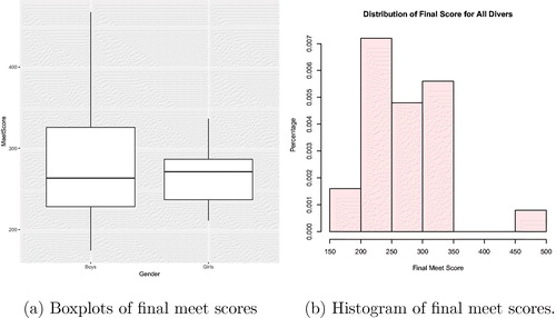
The diving data are a rich source of examples for visual representation, and two simple ways to explore the data are boxplots and histograms. Figure 1(a) shows a boxplot for the final scores separated by boys and girls, and Figure 1(b) is a histogram of the final meet scores. Even with data as complex as the diving data, analysts can learn from simple plots. In Figure 1(a), the side-by-side boxplots for the final meet scores for boys and girls show that the scores for boys vary more than those for girls. In addition, the median final meet score for the girls is slightly greater than that for the boys. The histogram (Figure 1(b)) indicates that most of the scores are clustered between 250 and 300. Figure 1(b) also illuminates a large outlier on the upper end of the scale. This outlier is due to the score of the boy who won the competition. His score was 467.1, which was more than 100 points better than the next highest score for both boys and girls.

Fig. 1 Visual representations of the final meet score.

The code that generated Figures 1(a) and (b) is given in the supplementary materials. All visual aids use the graphical package ggplot2 (Wickham 2016). Boxplots and histograms help analysts understand the overall distribution of the data. In addition, more complicated graphics can inform expectations for the results of an analysis, or on their own can answer questions about the data.

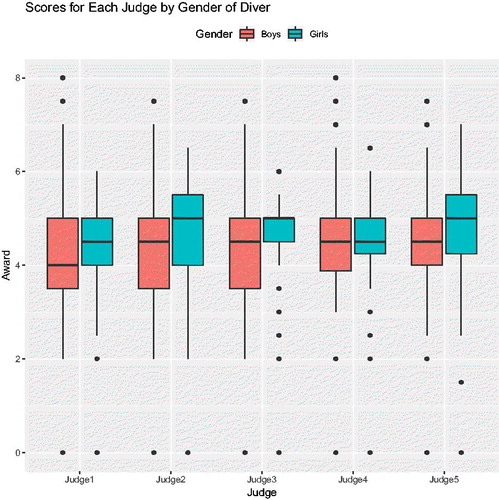
Boxplots of scores by gender and judge can also be helpful in exploring the data. Figure 2 shows the scores for each judge by gender of the diver. Scores for boys are shaded in coral, and scores for girls are shaded in teal. The boxes are grouped by judge, and each judge is labeled along the horizontal axis. In Figure 2, we can see that the pattern of having more variability in scores for boys is mainly due to judges 1, 2, and 3. Furthermore, judge 2 seems to have the most variability in scores. Except for judge 4, all judges give girls slightly higher median scores than they do for boys.

Fig. 2 Boxplots of judges’ scores by judge and gender of diver.

4.1 Creating Trajectory Plots

Because each round of dives represents a repeated measure for each diver, graphing the score by round for each diver may give more insight into the data than given in Figures 1 and 2. Figure 3 shows a plot for the score for each round on the vertical axis by the round number on the horizontal axis. Each diver is represented by a different line and color. Divers A to M are girl divers and divers N to Y are boy divers.

Fig. 3 Trajectories of round scores for each diver. Lines represent scores across rounds for each diver.

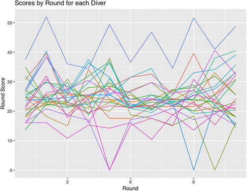
The plot in Figure 3 is aptly named a “spaghetti plot” because the lines resemble spaghetti in a bowl. The top diver, whose score corresponds to the outlier seen in Figure 1(b), stands out because his score is always above the score of every other diver. The figure also illuminates that four divers failed their respective dives (scores of 0) in different rounds. Furthermore, the dataset shows that rarely do divers score below 15 or above 35 for a given round. The trajectories of scores show no discernible pattern of increasing or decreasing between round 1 and round 11, although one could argue that there is a tendency for the last dive to be scored higher than the penultimate dive (“saving the best for last,” perhaps). Figure 3 also shows that round scores for girl divers tend to be lower than those of boy divers. Recall that DD is factored into the round score (Franklin 2018); therefore, differences may result from the DD for each dive.

Using Figure 3, it is difficult to use to follow the round score of a single diver. This difficulty is one of the limitations of a spaghetti plot. One way to simplify the plot and thus the process of following a single diver would be to separate the plots into facets, where each facet represents a value of a categorical variable. For this separation, an obvious variable to use is gender, as is done in Figure 4, which shows the trajectory plot from Figure 3 split by gender, with boys in the upper part of the graph and girls on the lower part.

Fig. 4 Trajectories of round scores for each diver by gender. Lines represent scores across rounds for each diver.

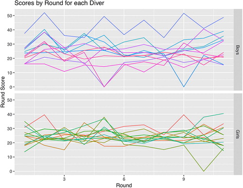
Whereas Figure 3 shows the range for all divers, the representation of the data in Figure 4 more clearly illustrates that the ranges for the boys’ scores are wider than those for the girls’ scores. The girls’ scores tend to be harder to distinguish in Figure 3 than are the boys’ scores.

Other ideas for plotting these data would be to plot cumulative scores for each gender, or to plot the round scores of the top half of the divers from each group, as determined by their final placement. The webpage (UCLA Statistical Consulting Group 2018) suggests more additions to trajectory plots for repeated measures data, including placement of average values for a group of variables.

4.2 Degree of Difficulty Versus Total Score

These data were originally gathered to answer the question of whether divers would score better if they perform easy dives well or more difficult dives less well. To answer this question with visual representation of the data, students need to add DD as a variable in the plots. The problem with DD is that not all divers perform dives with the same DD. Using only DD to separate the divers into facets, for example, could result in grids with only one diver represented. Students can solve this problem is by categorizing DD. For example, the following code creates a new variable called “DDfactor” that equals “High” if the DD for a dive is greater than or equal the median DD for all dives, which is 1.7, and “Low” otherwise. Mathematically, (1) $$\text{DDfactor}=\{\begin{array}{cc}\text{High}\hfill & \text{if}\text{DD}>1.7,\hfill \\ \text{Low}\hfill & \text{if}\text{DD}\le 1.7.\hfill \end{array}$$(1)

Students can experiment with various cutoffs, or even multiple cut-offs, in class to determine which cutoff renders the most interpretable results.

Figure 5 shows the final ranking of divers on the horizontal axis with the trimmed mean for the judges’ score for each round on the vertical axis. Figure 5(a) shows the girls’ scores and Figure 5(b) shows the boys’ scores. The trimmed mean was calculated by dropping the greatest and least judges’ scores for each round, and averaging the three middle scores. Each score is colored with gold for a difficult dive or blue for an easy dive.

Fig. 5 Average of middle three judges’ scores for each dive by place of the diver. Girls scores are on the left, boys on the right. Each dot represents a different judge’s score for a particular dive. Low DD dives ($\text{DD}\le 1.7$) are colored blue while high DD dives are colored gold.

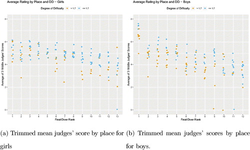
Each place corresponds exactly to one and only one diver; therefore, each point represents a different judge’s ranking for a given diver. The ordering of the scores by place allows for easier interpretation of the plot. In a first attempt of this plot, the ordering was done by diver instead of by place. This made the question of the effect of DD on place more difficult to answer. After discussing the problem of determining the effect of DD with diver on the x-axis, the students considering this dataset decided to use place on the x-axis instead, resulting in a cleaner interpretation for the plot. In this plot, we see that the top finishers received higher scores on easy divers than on difficult ones; however, they also attempted more difficult dives than those finishing in the bottom third of the competition.

Figure 5(b) illustrates that the boys’ best scores were for dives with low DDs. The scores for the first place diver are different, as he obtained high scores on all dives, regardless of DD. The diver in 10th place performed one high DD dive moderately well, but failed a dive and did not do as well on his lower difficulty dives. The 11th and 12th place divers had few difficult dives. These data highlight that difficult dives are important for doing well in the competition. However, the best divers seemed to perform their low DD dives better than their high DD dives. From Figure 5(b), the conclusion about DD and place is that a diver should concentrate on performing extremely well on low DD dives.

Results for girls (Figure 5(a)) are more mixed. For the top five girls, the dives are rated equally, regardless of the degree of difficulty. For girls in 7th place and below, the more difficult dives received lower ratings. Perhaps this reflects the fact that these particular girls were trying dives that stretched their ability. For both boys and girls, high DD dives are important, but the diver does not have to perform them as well as the lower DD dives to earn a high score in the competition.

4.3 Round Off Error in Final Scores

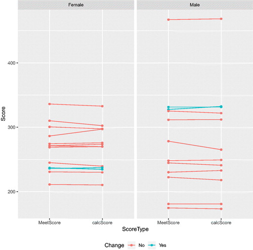
As stated earlier, the score for each diver in each round is the sum of the middle three judges’ ratings multiplied by the DD for that dive, and the final score is the sum of the 11 round scores, which have been rounded off before being added. To explore the effect of round-off error on final placement, the official meet score for close scores should be compared without being rounded off. In Figure 6, MeetScore was plotted versus the calculated meet score (calcScore) for both boys and girls. The score is connected by lines that represent the final ranking of the diver to which the scores correspond. Teal lines within the plot indicate a change in placement for those divers. For girls in the left panel of Figure 6, the fourth-place diver has a calculated score that is almost the same as the third-place diver. In fact, the third-place diver is still in third place, but only by 0.55 points (297.60–297.05). The calculated scores for the seventh- and eighth-place divers are separated by only 0.1 points (269.95–269.85) and the tenth- and eleventh-place divers change places when the score calculation is taken out to sixteen digits. For the boys, the second- and third-place divers exchange places, but this exchange does not affect whether these two divers are eligible to move to the next level; however, it does effect which diver obtains a silver medal and which the bronze. For this competition, the round-off error does not affect advancement to the next level, but the final scores are close and they give students an example of the impact of round-off error when making decisions.

Fig. 6 Official meet scores (with round off error) on the left versus calculated scores (no round off error) on the right for male and female divers. The lines connect scores corresponding to the same diver.

5 Diving Into Regression and Correlation

This section addresses regression and correlation to answer questions about the relationship of the DD to the final meet score and the effect of round-off error on the final placement and also to examine whether this effect is the same for boys and girls. To create a regression model, the first step is to examine the relationship between two quantitative variables via a scatterplot. From there, the analyst can determine the appropriate type of regression model for the data. This dataset has only one final meet score per participant (i.e., there are 25 final meet scores), yet the dataset potentially has 25 × 11 distinct values of DD for each diver. The word “potentially” is used because some divers may perform two or more dives that have the same DD. To examine the relationship between DD and final score, one solution is to obtain the mean (or median) DD for each diver and find its correlation with the final score. Another solution is to use all DD values and to calculate the correlation with the total score for each round and each diver. Yet another solution is to calculate the correlation of each DD with the average of the 20% trimmed mean of the judges’ scores for each round, as was used in Figure 5(b). Table 3 shows the Pearson and Spearman correlation coefficients of mean DD and final scores median DD and final score, and all DD values versus trimmed mean scores for both genders.

Table 3 Pearson and Spearman correlations for average DD and median DD versus 20% trimmed mean judges’ scores.

	Mean DD versus trimmed mean score		Median DD versus trimmed mean score		Rounds as Independent
Correlation	Boys	Girls	Boys	Girls	Boys	Girls
Pearson	0.669	–0.261	0.774	–0.461	–0.002	–0.311
Spearman	0.764	–0.401	0.781	–0.543	–0.044	–0.289

Interestingly, both the Pearson and Spearman correlation for all girls’ scores (in all three situations in Table 3) with DD are moderately negative. This would indicate that judges tend to give girls higher marks for less difficult dives. There are several ways to interpret these findings. One is that the judges tend to rate girls more harshly on difficult dives. It is also possible that the girls are better at easier dives. Finally, girls may be performing more difficult dives on average. The instructor should encourage the students to use to the data to determine which of these is most plausible.

The judge’s scores and the dives’ DD are on ordinal scales; technically, only the Spearman’s coefficient is appropriate for ordinal scales. However, theorists (Zumbo and Zimmerman 1993) have found that using measures meant for ratio or interval data, such as Pearson’s correlation coefficient, on ordinal data usually results in interpretable and useful values. An issue that arises from this calculation is if outliers are present in the data, indicated per the differences between the values of the coefficients. For example, the Pearson coefficient for the mean DD versus the final score for boys is 0.669 and the Spearman coefficient is 0.764. The smaller Pearson correlation coefficient could be due to an outlier. In analyzing the data, the Spearman’s correlation coefficient is more appropriate in the presence of outliers and data with nonlinear relationships.

To determine whether any differences are due to outliers or nonlinearity, a scatterplot is necessary. Scatterplots for all three pairs of variables are shown in Figure 7. Scatterplot matrices typically are difficult for students to interpret at first sight. However, once the plots are explained, students appreciate them for the amount of information that they display in a compact space. In Figure 7, the top row shows scatterplots with mean DD for all divers on the vertical axis, and the middle row shows two plots in which the median DD for each diver is represented on the vertical axis. The two plots in the bottom row each have the trimmed mean score on their vertical axes. Additionally, in Figure 7, values for the girls are depicted with coral circles, and values for boys are depicted using cyan squares.

Fig. 7 Average DD (top row), median DD (middle row), and final score (bottom row) for each diver. Boys’ scores are labeled with cyan squares and girls’ scores are labeled with coral circles.

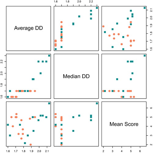
The bottom row of Figure 7 is the relevant row in this matrix, as it shows the relationships between the trimmed mean score and the mean or median DD. The bottom left and middle plots do not show much spread in the mean or median DD for girl divers. However, mean DDs for boy divers have more spread. Furthermore, the Pearson correlation is less than the Spearman correlation for boys because of the diver with the high DD and high score. This diver’s point lies outside the trajectory of the other points; thus increasing the variance in the denominator of the Pearson correlation coefficient and decreasing the overall correlation coefficient.

Students can use these data to obtain a model for the relationship between DD and final score.

6 Diving Into Interrater Agreement

Interrater agreement and rater bias have been explored many times in the literature (Emerson, Seltzer, and Lin 2009; Morgan and Rotthoff 2014; Kramer 2017; Looney 2012), particularly with respect to figure skating and gymnastics. In fact, the findings of judging bias have lead to changes in the scoring mechanisms used in both sports. The diving data do not lend themselves to exploration of judge bias because the affiliations of the judges and the affiliations of the divers are not known.

One of the first measures of interrater agreement was Cohen’s kappa (Cohen 1960), which measures the observed agreement between two raters, each of whom classify N participants into C categories. Cohen’s kappa is calculated using the simple formula (2) $$\widehat{\kappa }=\frac{p_0-p_c}{1-p_c},$$(2) where $p_{i·}={\sum }_{j=1}^C{p}_{\mathit{ij}}$ is the proportion of subjects classified into category $ı$ by rater one and $p_{·j}={\sum }_{i=1}^C{p}_{\mathit{ij}}$ denotes the proportion of subjects classified by rater two into category $\mathit{ȷ},i,j=1,\dots ,C$. Then, $p_o={\sum }_{i=1}^C{p}_{\mathit{ii}}$, which measures the proportion of times that the raters agree and $p_c={\sum }_{i=1}^C{p}_{i·}{p}_{·i}$, which measures the proportion of times agreement would occur by chance. Cohen’s kappa was originally meant for nominal data with a comparison of only two raters.

As a first step, students can take all of the judges’ scores (all 24 times 5 times 11 of them) and compute a kappa statistic for each of the 10 possible pairings of judges. However, there are some additional decisions to make before the kappa statistic can be computed. Because the kappa statistic is meant for nominal data, students will have to decide on a method for categorizing the ratings. For example, a ratings could be assigned for each round and each judge according to Table 4.

Table 4 Example method of assigning categories for computation of Cohen’s kappa.

Category	Low quality	Medium quality	High quality	Excellent
Judge’s rating	<3.5	4–5	5.5–6.5	>7

Students will likely discover that not all categories will have entries; therefore, the class will have to discuss issues of missing data. In addition, there will be tied observations (e.g., Judge 5 assigns several 5.5’s in Round 1). There are several common ways to deal with ties, such as use of mid-ranks (Kendall 1945) or omitting ties (Wilcoxon 1945). Class discussion can be centered around the merits and demerits of each method, and advanced classes can discuss less well-known methods of dealing with ties, such as those given in Student (1921) and Woodbury (1940).

In addition, once computed the kappa statistics will be difficult to interpret, due to the many comparisons to be made. The course instructor can then discuss the validity of the statistic and of the p-value that results from the test. This step is a good way to discuss assumptions of hypothesis tests and is also a segue into multiple comparison methods. From this discussion, students will identify that there are multiple raters, and that data are simply not suited for the kappa statistic, which leads into a discussion of measurement of agreement for multiple raters using ordinal or interval data.

Fleiss’ kappa was developed to examine agreement between multiple raters (Banerjee et al. 1999). Fleiss’ kappa is calculated with the following equation (3) $$\widehat{\kappa }=\frac{\sum _{i=1}^n\sum _{j=1}^m{K}_{\mathit{ij}}^2-K_n[1+(K+1)]\sum _{j=1}^m{p}_j^2}{\mathit{nK}(K-1)(1-\sum _{j=1}^m{p}_j^2)},$$(3) where $p_j=\frac{1}{K_n}{\sum }_{i=1}^n{K}_{\mathit{ij}}$, and K_ij is the number of raters who assigned the ith subject to the jth category, $i=1,\dots ,n,j=1,\dots ,m$.

Fleiss’ kappa is meant for nominal data. Therefore, with the diving data, the fact that the judges are giving measures on an ordinal scale leads to new levels of complexity, in terms of agreement, for ordinal and interval level data. One statistic that measures agreement for ordinal or interval data is the intraclass correlation coefficient (ICC). Let k be a fixed number of raters who judge n subjects. There are many different versions of ICC (Shrout and Fleiss 1979). ICC₃ is the version of ICC that is relevant for the diving study. It is given by (4) $${\text{ICC}}_3=\frac{\text{MSB}-\text{MSE}}{\text{MSB}+(\mathit{nk}-1)\text{MSE}},$$(4) where n = the number of participants, k = the number of judges. If we think of the calculation of judge agreement in terms of a two-way mixed ANOVA model with the random effect as judges (for one round) and divers as the fixed effect, MSB refers to the mean squared difference in scores between judges. In other words, it is the mean squared difference of each diver’s score for each judge from the mean score for each judge. MSE refers to the mean squared error. It is important to understand that the ICC₃ measures agreement between judges for each round separately. Therefore, for the diving data, we would have to calculate 11 ICC₃ values.

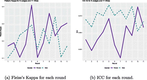
While measures of agreement for multiple raters exist, all of them assume that there is only one measured characteristic per subject. The diving data are different from other datasets used as examples for judge agreement in that the diving data involve multiple rounds of measurements in addition to multiple raters; however, this presents a valuable learning experience for students. Students can make their first attempt at dealing with multiple rounds by computing the statistic for each round and plotting the results. For example, in Figure 8(a), Fleiss’ kappa is plotted for each round and ICC is plotted for each round in Figure 8(b). In Figure 8, the solid purple line represents scores for girls and the green dashed line represents scores for boys; regardless of the measure of agreement, the figure shows that agreement is less variable and greater for boys than for girls. Students can also explore judges’ agreement for different DDs. Other questions for exploration with respect to rater agreement are given in the Appendix.

Fig. 8 Measures of agreement for each round. Agreement for girls is represented by the solid purple line and agreement for boys is represented by the green dashed line in both figures.

7 Diving Into Advanced Topics

The diving data are inherently multivariate due to the multiple rounds of scores for each diver. Therefore, the data lend themselves for students to use in multivariate statistics or in log-linear or ordinal modeling. The students could also discuss methods of including the multiple rounds of scores in an agreement measure, and adjusting that measure for covariates, such as gender of the diver, seed within the competition, and dive difficulty.

The data provide students with many kinds of bias to explore with regard to subjective ratings. Such biases include order bias (primacy and recency), reference bias, and difficulty bias (Kramer 2017; Morgan and Rotthoff 2014). Order bias is the notion that the order in which participants perform in a competition has an effect on the outcome. Reference bias is present when judges give favorable ratings to those contestants they recognize; the recognition may be due to diver reputation or shared affiliation. Difficulty bias involves judging more difficult routines (or dives) more favorably. Although none of these biases have been investigated in the diving dataset, more advanced students may find the investigation of these biases interesting and rewarding.

In addition to order bias in terms of the participants, in diving even the required dives are not required to be performed in a given order. For example, one diver may choose to perform a forward 1.5 in a pike position in the first round, whereas another diver may perform the same dive in the sixth round, and another diver may do the dive in a tuck position instead of a pike. Therefore, the judges are not actually scoring the same dive in each round for each diver; the round and the dive and the order are confounded. As a result, advanced students could also explore the effect of dive order on score.

As mentioned earlier, measures of agreement for multiple raters are available, yet none of them allow for multiple observations per subject in addition to multiple raters. One notable exception is Kraemer’s kappa (Kraemer 1980), which is not ideal for these data because its calculation requires ranking the response categories of the m_i measures for each subject i, with appropriate consideration of ties. The diving data includes many ties in the data, and not all of the possible “categories” of scores, from 0 to 10 by 0.5, are used (for 21 possible categories). These ties result in sparse data and an inaccurate measure of agreement. Furthermore, Kraemer’s kappa assumes that the m_i measures are independent, which is not true of the diving data. Nevertheless, advanced students can either code Kraemer’s kappa or modify it—for example, by grouping the 21 possible scores into three or four categories (e.g., high, medium, low, and fail) to calculate Kraemer’s kappa.

Advanced students can also consider various methods that explore the patterns of agreement in the dataset rather than a simple agreement statistic. Methods such as log-linear models (Graham 1995), latent class models (Agresti 1992), ordinal generalized linear mixed models (Nelson and Edwards 2015) and Bayesian ordinal models (Cao 2014) are all advanced models that can yield insight into not only whether the judges agree, but how they do so. Bayesian ordinal models and ordinal GLMMs were previously used on these data (unpublished analysis). The results indicated that Judge 1 tended to be stricter than the other judges and that all judges were better able to discriminate among male divers than they were among female divers.

Another advanced topic to explore is the effect of serial correlation on ratings and/or performance, and its consequences for measures of agreement. The effect of serial correlation has been considered in simulation studies, which indicate that the presence of dependence among observations has a detrimental effect on Type I and Type II error in ANOVA settings (Warner 2013). Students in an advanced course in statistical methods or statistical computation can explore the question of the effect of dependence among judges on the validity and reliability of hypothesis tests for various measures of agreement.

8 Conclusion

Students benefit when they use real data in statistical analysis. They also need to realize that not all data can be analyzed by “textbook” statistical methods. Students then can learn from the diving data, which gives them an opportunity to analyze a rich dataset through visual representation and nonstandard statistical methods.

Supplementary Materials

DivingData2018.xlsx data set of dives performed and scores for each diver for each of 11 rounds from a high school regional diving competition. These are the data used for this article. DivingDataRCode.txt: plain text file containing all R functions for the analysis, tables, and figures given in the paper.

Appendix: Questions for Further Consideration

1. Discuss whether the data constitute a sample or a population. What are the implications for analysis of each?

2. Discuss the level of measurement for the judges’ ratings. What statistical methods lend themselves to this level of measurement?

3. Explain the difference between treating each round as an observation and each diver as an observation. How does the choice impact the statistical analysis?

4. Are the diving data as entered “tidy,” as defined by Wickham (2014)? If so, explain why. If not, determine how they could be made “tidy.”

5. Plot the data for the girls and boys and determine if the relationship between DD and final placement are the same for the two groups.

6. Many researchers use Pearson’s or Spearman’s correlation coefficients to measure agreement between two measures gathered on an interval or ratio scale. Discuss the advantages and disadvantages of these approaches for the diving data.

7. Use scatterplots to interpret the correlation coefficient. Draw a scatterplot matrix of the relationships depicted in Table 3.

8. Discuss other categorical variables, or groupings of ordinal variables, that can be created to help answer specific questions about the round scores, final scores, or judges’ ratings.

9. Ask students to research interrater agreement in sports by looking at the controversies that led to changes in the scoring of figure skating and gymnastics competitions. Some helpful references are Brennan (2018), Pilon et al. (2018), Zaccardi (2012), and Smith (2018). Students may also want to examine interrater agreement in food competitions, such as wine tasting and chili cook-offs.

10. Examine whether interrater agreement differs by dive difficulty.

11. Most interrater agreement calculations assume that the raters (judges) are making their assessments independently of one another. In diving competitions, the judges sit in close proximity to one another, and scores are posted to the pool score board as they are entered into the electronic scoring system. Students can discuss if this method of displaying scores affects the assumption of independence.

References

- Agresti, A. (1992), “Modeling Patterns of Agreement and Disagreement,” Statistical Methods in Medical Research, 1, 201–218. DOI:10.1177/096228029200100205.
- Baker, B. O., Hardyck, C., and Petrinivic, L. F. (1966), “Weak Measurements vs Strong Statistics: An Empirical Critique of S.S. Stevens’ Proscriptions on Statistics,” Educational and Psychological Measurement, 26, 291–309. DOI:10.1177/001316446602600204.
- Banerjee, M., Capozzoli, M., McSweeney, L., and Sinha, D. (1999), “Beyond Kappa: A Review of Interrater Agreement Measures,” The Canadian Journal of Statistics, 27, 3–23. DOI:10.2307/3315487.
- Brennan, C. (2018), “U.S. Figure Skating Committee Picks Olympic Stars but Leaves Heartbreak in Its Wake,” USA Today, available at https://www.usatoday.com/story/sports/christinebrennan/2018/01/07/us-figure-skating-pyeongchang-controversy-ross-miner-adam-rippon/1011464001/.
- Cao, J. (2014), “Quantifying Randomness Versus Consensus in Wine Quality Ratings,” Journal of Wine Economics, 9, 202–213. DOI:10.1017/jwe.2014.8.
- Cohen, J. (1960), “A Coefficient of Agreement for Nominal Scales,” Educational and Psychological Measurement, 20, 37–46. DOI:10.1177/001316446002000104.
- Emerson, J. W., Seltzer, M., and Lin, D. (2009), “Assessing Judging Bias: An Example From the 2000 Olympic Games,” The American Statistician, 63, 124–131. DOI:10.1198/tast.2009.0026.
- Franklin, W. (2017), Calculating Degree of Difficulty for Dives: DD Formula in Springboard and Platform Diving, New York, NY: ThoughtCo, Inc.
- Franklin, W. (2018), High School Diving Competition Requirements, New York, NY: ThoughtCo, Inc.
- Gamer, M., Lemon, J., Fellows, I., and Sigh, P. (2012), “irr: Various Coefficients of Interrater Reliability and Agreement,” R Package Version 0.84 Edition.
- Graham, P. (1995), “Modeling Covariate Effects in Observer Agreement Studies: The Case of Nominal Scale Agreement,” Statistics in Medicine, 14, 299–310. DOI:10.1002/sim.4780140308.
- Kendall, M. G. (1945), “The Treatment of Ties in Ranking Problems,” Biometrika, 33, 239–251. DOI:10.1093/biomet/33.3.239.
- Kraemer, H. C. (1980), “Extension of the Kappa Coefficient,” Biometrics, 36, 207–216.
- Kramer, R. S. S. (2017), “Sequential Effects in Olympic Synchronized Diving Scores,” Royal Society Open Science, 4, 160812, 2017. DOI:10.1098/rsos.160812,.
- Lane, D. M. (2018), Online Statistics Education: A Multimedia Course of Study, Houston, TX: Rice University, available at http://onlinestatbook.com/.
- Looney, M. A. (2012), “Juding Anomalies at the 2010 Olympics in Men’s Figure Skating,” Measurement in Physical Education and Exercise Science, 16, 55–68. DOI:10.1080/1091367X.2012.639602.
- Morgan, H. N., and Rotthoff, K. W. (2014), “The Harder the Task, the Higher the Score: Findings of a Difficulty Bias,” Economic Inquiry, 52, 1014–1026, DOI:10.2139/ssrn.1555094.
- Nelson, K., and Edwards, D. (2015), “Measures of Agreement Between Many Raters for Ordinal Classification,” Statistics in Medicine, 34, 3116–3132. DOI:10.1002/sim.6546.
- Pilon, M., Lehren, A. W., Gosk, S., Sigel, E. R., and Abou-Sabe, K. (2018), “Think Olympic Figure Skating Judges Are Biased? The Data Says They Might Be,” Technical Report, NBC News.
- Prabhakaran, S. (2019), “Top 50 ggplot2 Visualizations—The Master List,” available at http://r-statistics.co/Top50-Ggplot2-Visualizations-MasterList-R-Code.html.
- R Studio (2019), “Tidyverse: R Packages for Data Science,” available at https://www.tidyverse.org/.
- Shrout, P. E., and Fleiss, J. L. (1979), “Intraclass Correlations: Uses in Assessing Rater Reliability,” Psychological Bulletin, 86, 420–428. DOI:10.1037/0033-2909.86.2.420.
- Smith, J. (2018), “Olympic Judging: Fair or Biased?,” Technical Report, Minitab.
- Student (1921), “An Experimental Determination of the Probable Error of Dr Spearman’s Correlation Coefficient,” Biometrika, 29, 322.
- UCLA Statistical Consulting Group (2018), “How Can I Visualize Longitudinal Data in ggplot2?,” available at https://stats.idre.ucla.edu/r/faq/how-can-i-visualize-longitudinal-data-in-ggplot2/.
- Velleman, P., and Wilkinson, L. (1993), “Nominal, Ordinal, Interval, and Ratio Typologies Are Misleading,” The American Statistician, 47, 65–72. DOI:10.2307/2684788.
- Warner, R. M. (2013), Applied Statistics: From Bivariate Through Multivariate Techniques (2nd ed.), Thousand Oaks, CA: Sage Publications, Inc.
- Wickham, H. (2014), “Tidy Data,” The Journal of Statistical Software, 59, 1–23. DOI:10.18637/jss.v059.i10.
- Wickham, H. (2016), ggplot2: Elegant Graphics for Data Analysis, New York: Springer-Verlag.
- Wickham, H. (2017), tidyverse: Easily Install and load the tidyverse.
- Wilcoxon, F. (1945), “Individual Comparisons by Ranking Methods,” Biometrics, 1, 80–83. DOI:10.2307/3001968.
- Woodbury, M. A. (1940), “Rank Correlation When There Are Equal Variates,” Annals of Mathematical Statistics, 11, 358. DOI:10.1214/aoms/1177731875.
- Zaccardi, N. (2012), “Scoring Controversy Takes Center Stage at Men’s Gymnastics Final,” Technical Report, Sports Illustrated.
- Zumbo, B. D., and Zimmerman, D. W. (1993), “Is the Selection of Statistical Methods Governed by Level of Measurement?,” Canadian Psychology, 34