Reading Versus Doing: Methods of Teaching Problem-Solving in Introductory Statistics

Abstract

Practice problems and worked examples are both well-established teaching techniques. Research in math and physics suggests that having students study worked examples during their first contact with new material, instead of solving practice problems, can be beneficial to their subsequent performance, possibly due to the reduced cognitive load required to study examples compared to generating solutions. However, there is minimal research directly comparing these teaching methods in introductory statistics. In this study, we chose six pairs of introductory statistics topics of approximately equal difficulty from throughout the semester. After an initial mini-lecture, one topic from each pair was taught using practice problems; the other was taught by having students read worked examples. Using Bayesian and frequentist analyses, we find that student performance is better after reading worked examples. This may be due to worked examples slowing the process of forgetting. Surprisingly, there is also strong evidence from in-class surveys that students experience greater frustration when reading worked examples. This could indicate that frustration is not an effective proxy for cognitive load. Alternatively, it could indicate that classroom supports during in-class problem-solving were effective in reducing the cognitive load of practice problems below that of interpreting written statistical explanations.

KEYWORDS:

• Cognitive load
• Practice problem
• Worked example

1 Introduction

Practice problems and worked examples are both well-established techniques for teaching problem-solving in statistics. Having students solve practice problems in class is a way to foster active learning, a key recommendation of the GAISE report (American Statistical Association 2016). Practice problems allow students to check their understanding of material, practice thinking statistically, and identify for themselves which aspects of a particular type of problem are most challenging. This can improve their interest in the material and their self-evaluation of their own understanding. In a study of 676 students, August et al. (2002) found that 91% of students from 4 departments at 7 institutions believed that they learned best through active participation. Titman and Lancaster (2011) found that graduate students in an epidemiology course reported that answering practice problems with a classroom response technology was an effective way to check their understanding. Zetterqvist (1997) reported that practice problems emphasizing real chemical data in a statistics course for chemistry majors improved students’ interest and motivation in the course. Similarly, Dexter et al. (2010) found that practice problems involving operating room management enhanced anesthesiologists’ perception that statistics was relevant to their careers. Carlson and Winquist (2011) found that a “workbook statistics” approach, in which students first solved problems individually or in groups, and then heard a brief summarizing lecture, increased students’ enjoyment of statistics and their self-evaluation of their own cognitive competence.

Practice problems have also been empirically associated with better performance. Giraud (1997) found that college students in an introductory applied statistics course who did practice problems in a group, in class, did better on exams than students who did the same problems individually outside of class. Vaughn (2009) found that graduate students in an introductory statistics course with a “balanced amalgamation” of mini-lectures and short active learning sessions performed better on the final examination than students in a lecture-only version of the course. They were also more likely to give the course an “excellent” rating for “communication of ideas,” “stimulation of interest,” and “facilitated my learning.” In mathematics, Rohrer (2009) reviewed a variety of articles that demonstrated higher exam scores among students from elementary school to college, who engaged in mixed practice of problems of multiple types and who spaced their practice over multiple days.

Having students read worked examples provides students with demonstrations of correct solution methods, which they can follow at their own pace. Worked examples allow students to compare and contrast problems that may be superficially similar, but structurally distinct, without the uncertainty of struggling to create a solution to a new type of problem. Quilici and Mayer (1996) found that college students who were given worked examples of t-tests, chi-square tests of independence, and correlation tests were more likely to sort new problems based on structural features (the type of test), while students who did not see the examples were more likely to sort problems based on surface similarities (the story context). Rinaman (1998) found that students at one school felt unsettled by the lack of worked examples in a workbook-style statistics textbook. Logically, the worked examples should be closely related to the desired educational outcomes: Layne and Huck (1981) found that providing examples of statistical computations to Master’s students in a research methods course did not improve students’ ability to interpret published research articles. Many textbooks are designed around the principle of providing students with worked examples (Atkinson and Renkl 2007). However, a common challenge is that students are reluctant to read the textbook outside of class, as Winquist and Carlson (2014) and Magalhães and Magalhães (2014) have noted in statistics, and others have noted in other fields (Clump, Bauer, and Bradley 2004; Berry et al. 2010). Moving the study of worked examples inside the class period could encourage students to take advantage of this learning opportunity.

Many studies have suggested that for problem-solving in math and physics, studying worked examples may be more effective than solving practice problems. Paas and Van Merriënboer (1994) found that Dutch college students who studied geometry problems and solutions simultaneously performed better on an immediate test of the material than students who were required to attempt to solve the problems before seeing the solutions. van Gog and Kester (2012) gave Dutch college students four problems involving electrical circuits, in either of two formats: alternating worked examples and practice problems, or four worked examples. They found no difference in performance on an immediate test, but found that the students who studied the worked examples performed better on a test one week later. Ringenberg and VanLehn (2006) found that for computerized homework assignments in introductory physics II, providing worked examples was more efficient than providing a series of hints which gradually increased in concreteness. Here, efficiency was measured by the number of problems a student needs to solve to achieve a given level of mastery on a post-test. Adaptive fading of worked examples, in which portions of the worked examples are converted to practice problems as students gain experience with the material, has been shown to provide benefits to performance in probability, geometry, and physics (electrical circuits) over practice problems alone (Renkl and Atkinson 2003; Salden et al. 2009).

Many researchers have hypothesized that superior performance using worked examples could be due to reduced cognitive load associated with studying the worked examples, compared to solving practice problems. Paas and Van Merriënboer (1994) found that students who studied worked examples reported significantly less perceived mental effort compared to students who attempted to solve problems. Tarmizi and Sweller (1988) found that when worked examples required students to divide their attention between two sources of information, students’ performance was no better than when solving practice problems without guidance. The cognitive load imposed by solving practice problems is higher for subject-matter novices than for experts, because experts typically possess schemas, complex memory structures that allow them to perceive complicated scenarios as a single unit (Atkinson et al. 2000). Therefore, researchers have hypothesized that the advantage of worked examples over practice problems is greater among novice learners. The term “novice learner” is somewhat vague; worked examples have been found to be superior to practice problems for learners as inexperienced as high school students (Paas 1992; Renkl and Atkinson 2003; Salden et al. 2009) up to college students as advanced as in the second semester of a 2-semester course sequence (Ringenberg and VanLehn 2006) or in their fourth year of vocational training (Paas and Van Merriënboer 1994). It may be more appropriate to classify students as novices based on their experience studying a particular topic or type of problem: In a study of Australian students in the first year of a trade course, Kalyuga et al. (2001) found that the advantage of worked examples diminished over a period as short as 2 or 3 weekly sessions of studying electrical relay circuits. This is consistent with the strategy of adaptive fading, as discussed by Renkl and Atkinson (2003) and Salden et al. (2009).

Despite extensive studies of worked examples versus practice problems in math and physics, these teaching methods have not been deeply compared in statistics. One study, by Paas (1992), found that high-school students who studied the concepts of mean, median, and mode via worked examples performed better on a subsequent test than students who studied by solving “conventional” problems, in which students were asked to generate the entire solution. This result agrees with results found in math and physics, but more research is needed to generalize it to college students and more challenging statistical concepts. In laboratory studies of college psychology students learning probability, Renkl et al. (2002) and Atkinson, Renkl, and Merrill (2003) compared the use of faded examples, with progressively more steps missing, to pairs of problems with one complete example and one practice problem. Both studies found that faded examples improved student performance later, on similar problems. While the topics of conditional probability and the general addition rule covered in these studies are important parts of many introductory statistics courses, we believe there is more to learn by comparing worked examples and practice problems across a range of topics in the introductory statistics curriculum. In addition, a study conducted in a semester-long statistics course complements laboratory studies, because it enables examination of students’ retention of material over a longer time period, in the context of the additional challenges of a typical course, such as students’ need to learn and retain a greater volume of related material.

In this study, conducted in a semester-long statistics course, we compared practice problems and worked examples for teaching a variety of introductory statistics topics. We chose six pairs of topics of approximately equal difficulty and randomly selected one topic from each pair to be taught using a combination of short lectures and reading worked examples. The other topic from each pair was taught using a combination of short lectures and problem-solving. We assessed student performance on selected quiz and exam questions, and we assessed students’ perceived learning, interest, and frustration using short questionnaires.

Below, in Section 2.1, we describe the data collection process. This includes the characteristics of the students and the overall structure of the course, as well as the specific practices used during class periods when practice problems or worked examples were employed as part of this study. To illustrate these practices, two of the lesson plans used in the study can be found in Appendix B. Section 2.2 explains our statistical methods. We conducted both a frequentist analysis (Section 2.2.1) and a Bayesian analysis (Section 2.2.2) of student performance, to investigate both the statistical significance of the effect size of worked examples, and its underlying distribution. Section 2.2.3 describes the statistical methods we used to analyze student perceptions of their learning, interest, and frustration. The results of our analyses are given in Section 3. Sections 3.1 and 3.2 correspond to the analyses described in Sections 2.2.1 and 2.2.2, respectively. Sections 3.3 and 3.4 contain the results of the analyses from Section 2.2.3. These results are divided into the relationship between the teaching method and the responses to each survey question separately (Section 3.3), and the relationships between responses to different survey questions (Section 3.4). In Section 4, we discuss how our findings relate to previous results from the literature on practice problems and worked examples. We also discuss limitations of this study, and suggest areas for further investigation.

The appendices contain examples of materials used in the data collection process. Appendix A contains the questionnaire used to assess students’ perceived learning, interest, and frustration. Appendix B provides detailed lesson plans for the topics from chapter 10 that were part of this study: the 1-proportion Z-test (taught by worked examples) and the 1-sample t-test (taught by practice problems). Appendix C contains the quiz and exam questions that were used to evaluate student performance for the topics from chapter 10. The worked examples and interpretation questions for all chapters are available at https://github.com/brisbia/Reading_vs_doing. The data and code used to conduct the analyses are also available at that site.

2 Methods

2.1 Data Collection

We compared two methods of teaching problem-solving in a single section of an introductory statistics course. The methods described below were approved by the University of Wisconsin-Eau Claire Institutional Review Board (application #BRISBIA44802015). We chose six pairs of topics, as shown in Table 1. Within each pair, the topics came from the same chapter of the course textbook, Statistics: Informed Decisions Using Data, 4th ed., by Michael Sullivan (Sullivan 2013). This textbook is required for the course; however, because pre-class reading is not assessed and homework is administered through WeBWorK (Gage, Pizer, and Roth 2002), many students rely primarily on their notes from class while studying. One topic from each pair was randomly chosen to be taught using practice problems, and the other topic was taught using worked examples. In three of the six chapters, the topics were covered in consecutive class periods; in the other three chapters, there was one class period between the coverage of the two topics. Because of weekends, the second topic was covered a maximum of four days after the first topic in the pair. These pairs of topics were chosen because we deemed them to be of approximately equal difficulty within each pair (as evidenced by their close proximity in the textbook and in the course schedule) and to involve similar types of problem-solving skills. For example, the topics in chapter 7 are both significantly reliant on effective use of calculators, while the topics in chapter 5 can both be solved using diagrams.

Table 1 Pairs of topics taught using practice problems and worked examples.

Chapter	Practice problems	Worked examples
5 (Probability)	General addition rule (Principle of inclusion-exclusion)	Conditional probability
7 (Probability distributions)	Computing probability from a normal distribution	Finding quantiles of a normal distribution
9 (Confidence intervals)	Confidence interval for a mean	Confidence interval for a proportion
10 (Hypothesis testing)	1-sample t-test	1-proportion Z-test
11 (Hypothesis tests for two samples)	2-sample Z-test of proportions	2-sample t-test
12 (Chi-squared tests)	Goodness-of-fit test	Chi-squared test of independence

NOTE: In each pair, the topic covered first is in bold.

This study was conducted in one section of introductory statistics in Fall 2015. The section included 60 students; 40 of these consented to have their quiz and exam scores included in the study. One student dropped the course, so the performance data analyzed below deals with 39 students. The course, and this study, includes primarily students between the ages of 18–22 years old. The course attracts students from a variety of majors, including nursing, kinesiology, and marketing. It fulfilled a requirement for the major of 17 of the 39 students who participated in the performance analysis. The fact that this was an introductory college course with diverse student majors is most similar to the study by van Gog and Kester (2012), discussed in Section 1, who studied students with a mean age of 20.65 years who had not taken science classes in their later years of secondary education. Twenty-eight (72%) of the students in our study had taken 2 or fewer semesters of college courses at the start of the semester. Therefore, in terms of being novice learners, our students fall in the middle of the pack relative to those in the studies discussed in Section 1. Because we used worked examples or practice problems during the first class period each topic was covered, all students were novices to the specific material, in the sense of Kalyuga et al. (2001).

All students in the course consented to fill out anonymous surveys about the teaching methods, so the data on self-assessments of learning, interest, and frustration below come from between 51 and 59 students for each chapter and method. Due to a lack of time in class, no survey was administered for the final chapter and method (chi-squared test of independence, taught by worked examples). All students in the course received the same instruction; therefore, the comparison of interest in this study is between topics within a section, not between different sections of students.

In each 50-min class period, the instructor (the first author) began the class with approximately 5 min of explanation about homework problems from previous class periods. The instructor then gave an initial explanation of the new topic, including demonstrating a worked example at the board. This mini-lecture lasted approximately 10 min. As an example, the mini-lectures and lecture examples for the topics in chapter 10 are provided in Appendix B. The remaining 35 min of the class period were devoted to one of two different treatments.

In sessions devoted to practice problems, the students were given problems to answer using iClickers, a classroom response technology. As an example, the practice problems about the 1-sample t-test, which was the chapter 10 topic taught using practice problems, are provided in Appendix B. Students typically solved the practice problems individually, using their notes from the preceding explanation by the instructor; some consulted the students sitting near them. These problems were designed to help students practice what had just been demonstrated as well as to give students experience with problems that extended or generalized what had just been demonstrated. For example, when teaching students how to compute probabilities from a normal distribution, the instructor demonstrated how to approximate the probability that a randomly selected bag of chocolate-chip cookies will have more than 1500 chocolate chips; students were then asked to approximate the probability that a randomly selected person will watch fewer than five hours of television per week. After students responded to the clicker question, the instructor revealed the correct answer and briefly demonstrated how to find it. Students were informed that 5% of their grades for the course were based on participation in responding to clicker questions, but that getting the correct answer did not affect their grades. Therefore, this constituted low-stakes immediate practice. Students worked on each problem until at least 50 out of the 60 students had entered a response using their iClickers and there had been no additional responses in the last 10 sec. This allowed the amount of time for each problem to vary from 2 to 6 min, based on the problem’s difficulty, while allowing leeway for absent students or those who forgot their iClickers on a particular day. The instructor then sometimes gave some additional explanation (less than 5 min) to prepare students for the next practice problem. This classroom structure was typical of most class periods in the course, not just those in which the study was being conducted.

In sessions devoted to worked examples, after the instructor’s initial explanation, students were given a handout with one or more example problems to read, broken into sub-problems where appropriate. Each example problem was followed by a written solution, approximately equivalent to what the instructor would say and write on the board if explaining the problem verbally. As an example, the handout about the 1-proportion Z-test, which was the chapter 10 topic taught using worked examples, is provided in Appendix B. The students were directed to read one portion of the handout at a time. After reading the explanation, students used iClickers to respond to questions about what they had just read. Some questions checked their understanding of what they read (“Which method did this example use to check for independence?”) while others asked them to evaluate (“In your opinion, what is the hardest part of this problem?”). The interpretation questions about the chapter 10 worked examples are included with the worked examples in Appendix B.

After each class period, students practiced each skill on homework assignments on the online system WeBWorK, which were due three times per week. Because students could seek help from the instructor, classmates, or the Math Lab on homework assignments, these were not used to evaluate student performance for purposes of this study. WeBWorK’s immediate feedback on correctness of each problem (on which students had unlimited attempts), along with the instructor-provided automated hints for selected questions, served as an important study aid for topics in both study treatments, in addition to the textbook and students’ notes from lecture.

Student performance was evaluated on selected quiz and exam problems, which were primarily short-answer questions. As an example, the quiz and exam questions used to evaluate student performance on the topics from chapter 10 are provided in Appendix C. For each question, the instructor graded the answers out of 2–6 points according to our usual practice in the course, but we then coded whether each response was “essentially correct” for purposes of this analysis. For most questions, a student could lose up to half a point due to minor arithmetic errors and still have an answer that was considered essentially correct. We opted to use a binary response variable, rather than the student’s percentage or points earned, because the quiz and exam questions had different point values and different rubrics, meaning that level of statistical mastery demonstrated by a score of 1 point or 50% (e.g.) was not consistent across questions. Each observation in the dataset represented a combination of one student and one quiz or exam question, resulting in a total of 1503 observations.

Student attitudes were evaluated using a brief questionnaire for each class period (see Appendix A). The survey assessed students’ perceived learning, interest, and frustration. Frustration was measured as one aspect of cognitive load (Haapalainen et al. 2010), with the idea that higher cognitive load could manifest as a feeling of being overwhelmed or “stuck” in understanding a problem.

Our intention was to administer the survey at the end of class; however, it was challenging to leave enough time at the end of class to distribute, fill out, and collect the survey. Therefore, most days, students filled out the survey at the beginning of the next class period. This could make the survey results less accurate than if they had been filled out immediately. Students completed each survey anonymously. This had the advantage of encouraging honest, unbiased responses, as students knew it was impossible for their grades to be penalized due to indicating a lack of interest in the class. However, it had the disadvantage of making it impossible to account for a student-level effect in the questionnaire responses, or to examine the association between perceived learning and actual performance.

2.2 Statistical Methods

Student performance was analyzed using both a frequentist and a Bayesian approach. These approaches take different, complementary perspectives on the nature of the effect of worked examples θ_M, as well as the other parameters we modeled (the effect of chapter, student, and time until assessment). The frequentist analysis treats θ_M as a fixed, unknown value; we use hypothesis tests to address the question “Is ${\theta }_M$ different from zero?” The Bayesian analysis treats θ_M as a quantity that can vary according to a probability distribution. We use Gibbs sampling to address the question “What is the distribution of ${\theta }_M$?”

The Bayesian approach is an effective way to represent the natural variability between sections of a statistics course. It is plausible that the effect size of worked examples (and the other parameters) would be somewhat different in another section of the same course, even one with very similar classroom procedures and student characteristics. Therefore, we can think of θ_M in our section of the course as being a random value drawn from the distribution of possible values of θ_M for all sections of introductory statistics with classroom procedures and student characteristics similar to this one. The Bayesian approach allows us to learn about that underlying distribution.

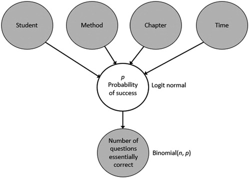
The Bayesian approach is also a useful means of expressing our mental model of a system of variables with multiple levels of influence: Student, chapter, teaching method, and time until assessment all influence the probability of success on a problem, which cannot be observed directly. In turn, the probability of success influences a student’s score on the problem, which we can observe. Our Bayesian hierarchical model (Figure 1) encodes these influences directly. It also allows us to directly model our uncertainty about parameter values via the prior probability distributions. Even when we do not wish to impose strong initial assumptions about a parameter’s distribution, as in this study, using different uninformative prior distributions allows us to evaluate the strength of the evidence in the data to overcome the uncertainty in the prior distribution. Additionally, using a prior distribution with a mean of zero, as we have done, results in shrinkage of parameter estimates (Gelman et al. 2004, p. 47), which is helpful in avoiding overfitting (Gelman et al. 2004, p. 117). This is particularly valuable for the by-student effects, where we are modeling many parameters (39 parameters, one for each student).

Fig. 1 Hierarchical Bayesian model of student performance.

2.2.1 Frequentist Analysis of Performance

For the frequentist approach, we used R versions 3.2.1-3.4.0 (R Core Team 2015–2017) to perform logistic regression of student performance. For each observation (combination of one student and one quiz or exam question), the dependent variable was coded as a 1 if the student’s response to the question was “essentially correct,” and a 0 if the student had errors other than minor arithmetic errors.

The predictors used in the logistic regression models are shown in Table 2. We examined a baseline model (Model 0) with method (worked examples or practice problems), student, and chapter. Models 1–6 also included time until assessment, the number of days between when the material was introduced in class and when it was assessed on the quiz or exam. Models 2–6 included an interaction term between time and method. Model 6 examined the effect of student characteristics by replacing the by-student factor with a set of 6 demographic variables (Table 3). In all of the models, chapter was treated as a factor variable.

Table 2 Summary of predictors used in frequentist models of student performance.

	Predictors in	Predictors selected by backward
Model	full model	stepwise regression
0	Method + student + chapter	Student + chapter
1	Time + method + student + chapter	Time + method + student + chapter
2	Time * method + student + chapter	Time * method + student + chapter
3	Time * method + student + chapter + 7 homework indicators	Time * method + student + chapter + Mean attempts on problems attempted at least once + Max attempts
4	Same as model 3, but without data from chapter 5: Time * method + student + chapter + 7 homework indicators	Time + method + student + chapter + Mean attempts on problems attempted at least once
5	Time * method + student + chapter + topic order	Time * method + student + chapter
6	Time * method + chapter + 7 homework indicators + 6 demographic variables	Time * method + chapter + Mean attempts on problems attempted at least once + Median attempts + Max attempts + Age + Transfer Credits

Table 3 Homework indicators and demographic variables used in Models 3, 4, and 6.

Homework indicators	Demographic variables
Percentage of homework problems completed successfully	Sex
Mean number of attempts among problems which the student attempted at least once	Age
Median number of attempts among problems which the student attempted at least once	Number of semesters at the current institution that the student had completed at the start of Fall 2015
Percentage of homework problems completed successfully among problems attempted at least once.	Number of transfer and Advanced Placement (AP) credits
Maximum number of attempts	Whether the student had previously taken a college-level math course
Mean number of attempts on all problems	Whether introductory statistics was required for the student’s major
Median number of attempts on all problems

Models 3, 4, and 6 also included seven indicators of student persistence and success on the homework (Table 3). Each indicator was computed based on homework problems that were due on or before the day of the quiz or exam. To reduce multicollinearity among these variables, each homework indicator was regressed on the set of variables appearing below it in Table 3, and the residuals were used as predictors. The median number of attempts on all problems was used without transformation.

After building each of the full models described in Table 2, we applied backward stepwise logistic regression to select a set of predictors that minimized Akaike’s information criterion (AIC). In Models 3, 4, and 6, it was necessary to omit some incomplete cases from the dataset (less than 5% of the cases). For purposes of comparing AIC between models, the selected versions of Models 1, 2, 3, and 6 were then refit on the set of 1473 cases with no missing data in any of the variables included in the final versions of those models.

A limitation of conducting the current study in a real classroom is that the topics in each pair may not be of exactly equal difficulty. In particular, conditional probability, the chapter 5 topic taught using worked examples, has a reputation for being a particularly challenging topic in introductory statistics. While we are not aware of any formal comparison of the relative difficulties of conditional probability and the general addition rule, the topic of conditional probability can be challenging to connect with statistical inference (Rossman and Short 1995) and with students’ intuitions (Keeler and Steinhorst 2001; Ancker 2006). Therefore, we analyzed student performance both with and without data from chapter 5. The only difference between Models 3 and 4 is that Model 4 excludes chapter 5.

In this study, topics were taught in the order in which they appeared in the course textbook, and which topic was taught using each method was randomly selected. This resulted in practice problems being used as the first method in 4 chapters, and worked examples as the first method in 2 chapters (Table 1). It is possible that the second topic in each chapter might be easier than the first topic, because students have previous experience with solving problems of a similar type. To account for this possibility, Model 5 included topic position (first or second) as a predictor.

2.2.2 Bayesian Analysis of Performance

For the Bayesian approach, a hierarchical model was used (see Figure 1). We modeled each student’s score as following a binomial distribution with parameters p_ijkd, the probability of success, and n_ijkd, the number of problems attempted. Here, i is the number of the student, j is the method (1 for practice problems, 2 for worked examples), k is the chapter, and d is the number of days until assessment. The prior distribution of $p_{\mathit{ijkd}}$ was$$p_{\mathit{ijkd}}\sim \text{logit} \text{Norm}\left(\text{mean}={\mu }_{\mathit{ijkd}},\text{variance}={\sigma }^2\right).$$

The precision, or inverse variance, parameter had an uninformative gamma hyperprior:$${\sigma }^{-2}\sim \text{Gamma}\left(\text{shape}=0.01,\text{rate}=0.01\right).$$

The mean was modeled as a sum of the effects of student, method, chapter, and days until assessment:$${\mu }_{\mathit{ijkd}}={\theta }_{S,i}+{\theta }_M{I}_{j=2}+{\theta }_{C,k}+{\theta }_{D}d,$$where ${\theta }_{S,i}$ is the effect of student i; θ_M is the effect of the worked examples; $I_{j=2}$ is an indicator variable which equals 1 for worked examples; ${\theta }_{C,k}$ is the effect of chapter k; and ${\theta }_D$ is the additive effect per day until assessment. All of the θ parameters were given a Normal hyperprior distribution with mean 0 and variance 10. The mean of 0 reflects a prior model in which each of the predictor variables (student, method, chapter, and time) is equally likely to have a positive effect as a negative effect. The variance of 10 was chosen to provide a relatively uninformative prior distribution, reflecting a lack of certainty about the values of the θ parameters. We also examined the sensitivity of the results to the choice of priors for the θ parameters using a variance of 1 (more informative) and 100 (less informative).

The model was implemented in WinBUGS (Lunn et al. 2000). We used 4000 iterations of burn-in and 50,000 iterations of sampling for each of three chains. Gelman–Rubin statistics of approximately 1.0 and Monte Carlo error of less than 5% of the standard deviation for each parameter indicated that the burn-in and sampling time were sufficient.

To allow for the possibility of conditional probability being harder than the general addition rule, we performed the Bayesian analysis both with and without data from chapter 5. To investigate the possibility that the second topic in each chapter might be easier than the first topic, we did a subset analysis of student performance on the groups of chapters in which each method was taught first. The worked examples-first analysis included only the data from chapters 9 and 10, while the practice problems-first analysis included chapters 5, 7, 11, and 12. If the second topic in each chapter is easier than the first, then we expect the advantage of worked examples to appear larger in the practice problems-first analysis, in which the effect of worked examples would be confounded with the effect of being the second topic.

2.2.3 Student Perceptions

The survey questions about interest, perceived learning, and frustration were analyzed in a variety of ways. For each question, we performed a two-sided test of proportions, grouping the top two categories of answers (“agree or agree strongly” or “a fair amount or a lot”). For interest and perceived learning, we also tested the proportion of questionnaires with the top answer category alone. This analysis was omitted for frustration, because only 2 out of 595 questionnaires during the semester reported “strongly agreeing” to the statement, “I felt frustrated during today’s class.” Because we did not have questionnaires from the worked examples lesson from chapter 12, we performed each test of proportions twice, once with and once without the data from chapter 12. The results were similar in either case.

To account for potential differences between chapters, we also used three regression models: two logistic and one linear model. All of the regression models used chapter and method (worked examples vs. practice problems) as predictors. The two logistic models used a response of 1 for survey responses in the top two categories or in the top single category, like the tests of proportions. The linear model measured survey responses on a scale from 0 (“disagree strongly”) to 4 (“agree strongly”) or a scale from 0 (“nothing”) to 3 (“a lot”). For the linear model, residuals were modeled as normally distributed. Because the survey responses were typically integers, we also tested generalized linear models with Poisson-distributed errors, but found these to produce a worse fit (as measured by AIC) and minimal difference in the conclusions. Because the surveys were completed anonymously, there was no way to pair questionnaires between the two treatments (teaching methods).

On six surveys out of 595, students circled both “a fair amount” and “a lot” in answer to the question about perceived learning; on one survey, a student circled both “a little” and “a fair amount”. These responses were counted as 2.5 and 1.5, respectively, for the linear regression. For the tests of proportions and logistic regression, these responses were rounded down to the lower of the circled categories.

We also examined the relationships between the responses to different survey questions in two ways. First, we used a chi-squared test of independence for each pair of survey questions, with and without the responses from chapter 12. Because only four questionnaires reported learning “nothing,” these responses were grouped with the questionnaires that reported learning “a little.” For interest level and frustration, the pairs of responses “Agree or agree strongly” and “Disagree or disagree strongly” were grouped to produce 3 categories for each variable. We also performed a linear regression of perceived learning on frustration and on interest level, and a linear regression of frustration on interest level, using chapter and method as additional predictors.

3 Results

3.1 Frequentist Analysis of Performance

In the baseline model (Model 0), there was no evidence that worked examples were associated with success (p-value = 0.43). However, this changed when time until assessment was included as a predictor. All six of Models 1–6 had odds ratios significantly less than 1 for time until assessment (Table 4), indicating that longer delays between learning the material and being tested on it are associated with lower probabilities of success. All of Models 1–6 also had odds ratios significantly greater than 1 for either worked examples, or for a time-by-worked examples interaction term, if such a term was included in the selected model. This indicates that when time until assessment is held constant, worked examples are associated with higher probabilities of success. The odds ratios above 1 for the time-by-worked examples interaction terms suggest that worked examples may slow the process of forgetting, mediating the negative effect of time until assessment.

Table 4 Odds ratios, p-values, and AIC of models for performance, selected by backward stepwise regression.

		Worked	Time:worked
Model	Time	examples	examples	AIC
1	0.9718	1.450 (0.0134)	NA	1288.43
	$\left(4.50\times {10}^{-12}\right)$
2	0.9645	1.065 (0.7661)	1.014 (0.0409)	1285.62
	$\left(7.61\times {10}^{-11}\right)$
3	0.9619	0.9765 (.9131)	1.015 (0.0398)	1271.97
	$\left(5.90\times {10}^{-12}\right)$
4	0.9696	1.476 (0.0317)	NA	–
	$\left(1.36\times {10}^{-6}\right)$
5	Same as Model 2	Same as Model 2	Same as Model 2	Same as Model 2
6	0.9645	0.9375 (0.7571)	1.014 (0.0364)	1316.91
	$\left(1.11\times {10}^{-11}\right)$

NOTE: Odds ratios are reported first; p-values are in parentheses. p-values less than 0.05 are indicated in bold or by scientific notation. In each model, the response variable was coded as a 1 if the student’s response to the question was essentially correct, and a 0 if the student had errors other than minor arithmetic errors. Models 2 and 5 had identical selected models. Coefficients are based on the largest dataset with no missing data in the variables included in the selected model; AIC is based on a common set of 1472 complete cases. Model 4 was fit to a smaller dataset than the other models, so its AIC cannot be compared with the AIC of different models.

The odds ratios for days until assessment and the time-by-worked examples interaction are close to 1. This indicates that in a single day, students forget relatively little, and they would derive little or no benefit from worked examples if they were quizzed the day after learning the material. However, in practice, we are interested in improving student performance long-term. For a quiz conducted 14 days after the material was introduced in class (the median in this study), Model 3 yields a net odds ratio of worked examples equal to $0.9765\times {1.015}^{14}=1.20.$ Moreover, the response variable in these models was performance on a single quiz or exam question. In the context of a semester-long course with weekly quizzes and multiple exams, a small improvement in a student’s probability of success on each problem could have a large impact on the student’s overall performance in the course. Therefore, we believe that the effects of time until assessment and the time-by-worked examples interaction shown in Table 4 have substantial practical significance, in addition to their statistical significance.

Model 3: When accounting for homework performance, the model selected by backward stepwise logistic regression included the maximum number of attempts and the mean number of attempts on problems attempted at least once, in addition to the predictors in Model 2. The mean and maximum number of attempts on homework were both significantly associated with success on quizzes and exams (Table 5). The maximum number of attempts was associated with an increased probability of success, while the mean was associated with a decreased probability. This could indicate that students who are successful on quizzes and exams tend to be persistent on homework, as evidenced by being willing to make many attempts on a particularly difficult homework problem. However, students who need to make many attempts on most of the homework problems, resulting in a large mean, may not be learning effectively from that experience. This model had the lowest AIC of Models 1, 2, 3, and 6, indicating that homework performance is a valuable predictor of success on quizzes and exams.

Table 5 Homework indicators included in Model 3.

Variable	Odds ratio	p-value
Mean attempts on problems attempted at least once	0.6738	0.0030
Max attempts	1.126	0.0066

NOTE: The response variable was student performance on a single quiz or exam question, coded as a 1 if the student’s response to the question was essentially correct, and a 0 if the student had errors other than minor arithmetic errors. p-values less than 0.05 are indicated in bold.

Model 4: When chapter 5 was excluded from the analysis, the results corroborated those of Model 1. This indicates that the overall conclusion of a beneficial effect of worked examples is not dependent on the relative difficulty of conditional probability and the general addition rule. Unlike in Model 2, for Model 4 the interaction term was not included in the model with the lowest AIC, although the model with an interaction term was a reasonable alternative, with AIC within 2 of the selected model.

Model 5: When topic order was included as a predictor in the initial model, it did not persist as a predictor in the model selected by backward stepwise regression. This meant that the final version of Model 5 was identical to Model 2. However, the model with topic order had an AIC of 1287.16, within 2 of the AIC of Model 2. In the full model, the odds ratio of topic order was not significantly different from 1 (p-value = 0.522), indicating a lack of evidence that students find the second topic in a chapter easier than the first. This may be due to the fact that student performance was assessed between 2 and 79 days after students were introduced to each topic. Students had a chance to solidify their understanding of each topic by practicing it on homework, which could reduce any advantage of immediate familiarity with a topic gained for the second topic in a chapter.

Model 6: When demographic variables were used instead of a by-student factor, the model selected by backward stepwise regression included two of the six initial demographic variables: age and number of transfer and AP credits (Table 6). A greater number of transfer and AP credits was associated with an increased probability of success, perhaps indicating a positive effect of greater intellectual maturity. This effect is small; the effective odds ratio associated with taking a single additional 4-credit course is ${1.012}^4=1.05.$ This is not surprising, given that students’ transfer and AP credits came from a wide variety of courses, not just courses related to statistics.

Table 6 Demographic variables included in Model 6.

Variable	Odds ratio	p-value
Age	0.9055	0.0019
Transfer and AP credits	1.012	0.0012

NOTE: The response variable was student performance on a single quiz or exam question, coded as a 1 if the student’s response to the question was essentially correct, and a 0 if the student had errors other than minor arithmetic errors. p-values less than 0.05 are indicated in bold.

Surprisingly, age was associated with a decreased probability of success. This suggests that, between two hypothetical students who entered our institution with the same amount of college-level experience (as measured by transfer and AP credits), the younger student may have a stronger academic background prior to college. The younger student is more likely to have taken AP courses, rather than to have transferred from a community college. In this dataset, age and number of transfer and AP credits were moderately correlated ($r=0.58)$. However, both the full model and the model after backward stepwise regression had all variance inflation factors less than 2, indicating that multicollinearity was not a problem.

Model 6 had an AIC of 1316.91, while Model 3, the equivalent model with a by-student factor, had an AIC of 1271.97. This indicates that the extra complexity of the by-student factor is warranted by its improved fit to the data. The six demographic variables used to construct Model 6 are not sufficient to predict the idiosyncrasies of each student’s baseline probability of success.

As in Model 3, the model selected by backward stepwise regression included the mean and maximum number of homework attempts. Model 6 also included the median number of homework attempts.

3.2 Bayesian Analysis of Performance

The Bayesian analysis supported the results of our frequentist analysis. The parameter θ_M had a mean and median of 0.40 and a 95% credible interval (CI) of (0.086, 0.724), indicating that worked examples had a positive effect. The 95% credible interval of θ_D was (–0.0389, –0.0220), indicating that the per-day effect of time until assessment was negative. These results were robust to the choice of hyperpriors, as shown in Table 7.

Table 7 95% credible intervals found with different hyperpriors.

Prior distribution for θ parameters	95% CI for θM	95% CI for θD
Normal$\left(\mu =0,{\sigma }_{\theta }^2=10\right)$	(0.086, 0.724)	(–0.0389, –0.0220)
Normal$\left(\mu =0,{\sigma }_{\theta }^2=1\right)$	(0.094, 0.695)	(–0.0363, –0.0201)
Normal$\left(\mu =0,{\sigma }_{\theta }^2=100\right)$	(0.096, 0.724)	(–0.0391, –0.0223)

NOTE: θ_M is the effect of worked examples; θ_D is the additive effect per day until assessment. The same prior distribution was used for each of the parameters ${\theta }_0,{\theta }_M,{\theta }_D,{\theta }_{C,k},$ and ${\theta }_{S,i}$.

Results of the subset analyses are summarized in Table 8. When chapter 5 was excluded from the analysis, we found a 95% CI for θ_M of (0.125, 0.876). This interval is shifted slightly to the right, compared to the interval when all of the chapters are included. This indicates that the average effect of worked examples is slightly larger when excluding conditional probability, which was taught using worked examples. This agrees with the hypothesis that students find conditional probability more challenging than the general addition rule. However, the interval still has substantial overlap with the intervals found from analysis of the entire dataset, indicating general agreement about the range of plausible effect sizes of worked examples. Crucially, the 95% CI without chapter 5 still indicates a positive effect of worked examples.

Table 8 95% credible intervals and central tendency for the effect of worked examples $\left({\theta }_M\right)$ using subsets of the data.

		Mean and median
Chapters used	95% CI for θM	of θM
All	(0.094, 0.695)	0.40
Exclude conditional probability: 7, 9, 10, 11, 12	(0.125, 0.876)	0.49
Worked examples first: 9, 10	(0.06883, 1.269)	0.66
Practice problems first: 5, 7, 11, 12	(–0.08155, 0.8242)	0.35

The 95% CIs from the worked examples-first (just data from chapters 9 and 10) and the practice problems-first (just chapters 5, 7, 11, and 12) subset analyses are shown in Table 8. These are wider than the interval from the full data analysis, as expected due to the smaller amount of data. However, there is substantial overlap with the interval from the full analysis. The worked examples-first analysis agrees with the conclusion that the effect of worked examples is positive. The 95% CI from the practice problems-first analysis allows for a small probability of a negative effect from worked examples; in the post-burn-in iterations, θ_M was positive 94.5% of the time.

Based on the hypothesis that the second topic in each chapter is easier than the first, we expected the advantage of worked examples to appear larger in the analysis of chapters 5, 7, 11, and 12, in which practice problems were used for the first topic and worked examples for the second. Interestingly, our results contradicted this expectation: The analysis of chapters 5, 7, 11, and 12 (practice problems first) had a mean of θ_M of 0.35, a less pronounced effect than in the full analysis (with a mean of 0.40). Meanwhile, the analysis of chapters 9 and 10 (worked examples first) had a mean of θ_M of 0.66, a more pronounced effect. This could indicate a primacy effect, making the first topic in a chapter easier to remember. Alternatively, it could support the claim that worked examples are most effective for novice learners: after students have gained the experience of one class period learning about a general type of problem, worked examples may be slightly less effective. Additional studies, with each topic within a chapter being taught both first and second to different subsets of students, would be valuable for determining whether this worked example × topic order effect is statistically significant.

3.3 Student Perceptions

Because we had no questionnaires from the worked examples lesson from chapter 12, we analyzed the questionnaire data twice, once with and once without the data from chapter 12. The results were very similar, with one exception (proportion who reported learning “a lot”). The results from the data including chapter 12 are summarized in Table 9.

Table 9 Summary of estimated coefficients and p-values from student attitudes survey data.

Variable	Linear model: coefficient of worked examples (p-value)	Logistic model: odds ratio of worked examples, focusing on top category (p-value)	Logistic model: odds ratio of worked examples, grouping top two categories (p-value)	Test of proportions: p-value, focusing on top category (“a lot” or “agree strongly”)	Test of proportions: p-value, grouping top two categories (“a fair amount or a lot” or “agree or agree strongly”)
Interest level	–0.1234	0.6622	0.7573	0.197	0.2021
	(0.0715)	(0.1924)	(0.1273)
Perceived	–0.07292	0.6986	0.8746	0.02762	0.9565
learning	(0.1547)	(0.0843)	(0.6322)
Frustration	0.3235	*	3.515	*	0.0020
	($6.85\times {10}^{-7}$)		(0.00152)

NOTE: Coefficients, odds ratios, and p-values listed are based on data including chapter 12. The linear and logistic models include chapter as a factor variable. The linear model uses normally distributed errors. No result is reported for frustration focusing on the top category, because only 2 out of 595 questionnaires during the semester reported “strongly agreeing” to the statement, “I felt frustrated during today’s class.” p-values less than 0.05 are indicated in bold or by scientific notation.

Students’ reported interest levels were approximately the same for both teaching methods. When chapter was included as a predictor, there was a weak suggestion of lower interest in worked examples (p-value = 0.07 for the linear model; p-value = 0.13 for the logistic model of “agree” or “strongly agree”).

More students said they learned “a lot” using practice problems (28% vs. 20%, p-value = 0.03) than worked examples; however, the strength of this result diminished when chapter 12 was excluded (p-value = 0.11). There was no statistically significant difference between the methods in the proportion who said they learned “a lot” or “a fair amount” (p-value = 0.96 with chapter 12, 0.76 without). Results of the logistic model, which included chapter as a factor, corroborated these results.

Interestingly, students were more likely to feel frustrated with worked examples (p-value = 0.002 for a 2-sided test of the proportion who “Agree or agree strongly,” regardless of whether chapter 12 was included). This result persisted in the logistic model, where chapter was included as a factor (p-value = 0.002). This contradicts the idea of practice problems involving greater cognitive load. This frustration could be due to confusion while trying to understand the written examples. It could also be due to boredom; as discussed in Section 3.4, frustration was associated with lower reported interest.

3.4 Relationships Between Student Perceptions

All three pairs of variables of student perceptions were significantly associated (Table 10). The associations were consistent regardless of the method of analysis and whether data from chapter 12 was included. Perceived learning was significantly associated with lower frustration and higher interest (p-values $\le 1.5887\times {10}^{-15}$; see Figures 2 and 3). Boredom was also significantly associated with higher frustration (p-values $\le 1.147\times {10}^{-10};$ see Figure 4).

Fig. 2 Relative frequency of frustration level as a function of perceived amount learned.

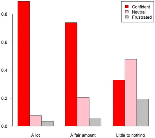
Fig. 3 Relative frequency of interest level as a function of perceived amount learned.

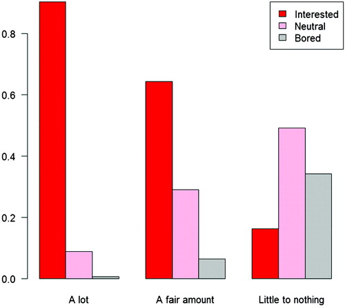
Fig. 4 Relative frequency of frustration level as a function of interest level.

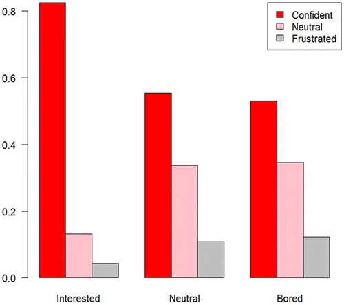
Table 10 Summary of estimated coefficients and p-values for relationships between student perceptions from questionnaires.

		Linear model:	Chi-squared test of
Perception	Perception	coefficient of	independence:
variable y	variable x	x (p-value)	p-value
Interest level	Perceived learning	0.6858	$1.4627\times {10}^{-28}$
		$\left(6.6500\times {10}^{-41}\right)$
Perceived learning	Frustration	–0.2612	$1.5887\times {10}^{-15}$
		($2.4956\times {10}^{-16}$)
Interest level	Frustration	–2.992	$1.147\times {10}^{-10}$
		($3.1358\times {10}^{-12}$)

NOTE: Coefficients and p-values listed are based on data including chapter 12. The linear models include chapter and method (worked examples vs. practice problems) as factor variables. The linear models use normally distributed errors. Coefficients with p-values less than 0.05 are indicated in bold.

4 Discussion

In this study, frequentist and hierarchical Bayesian analyses found better student performance for material that students learned through lecture + reading worked examples compared to material that students learned through lecture + solving practice problems. This agrees with the results of Paas (1992) among high-school students learning descriptive statistics, and with the results of Renkl et al. (2002) and Atkinson, Renkl, and Merrill (2003) among college students learning probability in a laboratory setting. Therefore, we have found evidence that the advantage of worked examples also applies to college students in the setting of a semester-long introductory statistics course. In the frequentist analysis, the difference between worked examples and practice problems was only apparent when the amount of time between learning and assessment was included in the model. This suggests that worked examples may slow the process of forgetting. This is consistent with the results of van Gog and Kester (2012), who found no difference in performance on an immediate test of students’ understanding of electrical circuits, but found that the students who studied the worked examples performed better on a test one week later.

We did not find evidence that the second topic in each chapter was easier than the first. A Bayesian analysis found a higher mean effect of worked examples on a subset of the data in which worked examples were taught first. This could indicate a primacy effect. It could also support the claim that worked examples are most effective for students who are novices to the material in a given chapter. It would be valuable to conduct additional studies to investigate these possibilities.

Creating worked examples was more time-consuming for the instructor than preparing practice problems. Each solution had to be written out in full detail, whereas when preparing practice problems, abbreviated notes were sufficient to remind the instructor of the key points to explain. To save time for other instructors, we have provided the full text of our worked example handout for chapter 10 in Appendix B; the worked example handouts for the other chapters are available at https://github.com/brisbia/Reading_vs_doing. Worked examples could also be used for other topics by asking students to bring their textbooks to class and read specific examples during class. With this strategy, the instructor would only need to prepare the interpretation questions for students to discuss and answer about each example.

In this course, topics that were not part of this study were taught using a class structure similar to that used for the practice problems treatment in this study. This could influence the results; for example, perhaps students remembered the worked examples better because they stood out as having been taught in an “unusual” way. Having observed the educational benefits of worked examples in this course, it would be valuable to increase the proportion of topics taught via worked examples and investigate whether the effects of worked examples remained the same.

Initially, we anticipated that students would experience frustration primarily as a result of feeling overwhelmed, confused, or “stuck” when solving a practice problem. Surprisingly, students were more likely to report frustration during class periods featuring worked examples. This could indicate that frustration was not an effective proxy for cognitive load. Because surveys were administered at the end of the class period or the beginning of the following class, frustration could reflect an overall dissatisfaction with the class period, rather than cognitive load in the moment of solving or reading a problem. In the future, it would be valuable to assess students’ frustration and/or perceived mental effort at various times throughout the class period, perhaps via classroom response technology.

Alternatively, lower frustration during practice problems could indicate that classroom supports, including the opportunity to discuss practice problems with peers, were effective in reducing the cognitive load of practice problems below the cognitive load of interpreting written statistical explanations. This could be the case, for example, if students experienced difficulty with reading comprehension, which Magalhães and Magalhães (2014) noted as a barrier to reading statistics problems. Given this, it could be valuable to examine whether students’ frustration is lower when watching videos of worked examples.

We found strong evidence of associations between students’ perceived learning, interest, and frustration levels. This corroborates the findings of Shernoff et al. (2003) among high school students, who found that students reported greater interest levels when participating in challenging activities, provided that their skills were appropriate to the challenge. In the future, it would be valuable to investigate the relationship between these student attitudes and student performance via the use of non-anonymous surveys.

Funding

This work was supported by the Wisconsin Teaching Fellows and Scholars Program of the University of Wisconsin Office of Professional and Instructional Development.

Appendix A

Student Attitudes Survey

Please rate how much you learned in today’s class:

Table

0	1	2	3
nothing	a little	a fair amount	a lot

Please rate how much you agree or disagree with the following statements:

Today’s class kept my interest.

Table

disagree		neither agree		agree
strongly	disagree	nor disagree	agree	strongly

I felt frustrated during today’s class.

Table

disagree		neither agree		agree
strongly	disagree	nor disagree	agree	strongly

Fig. A.1 Normal probability plot of simulated credit score data.

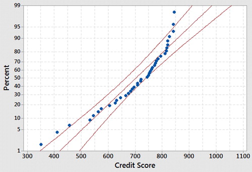
Fig. A.2 Minitab output from t-test of credit scores.

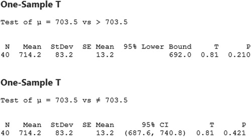
Fig. A.3 Boxplot and normal probability plot of holiday spending.

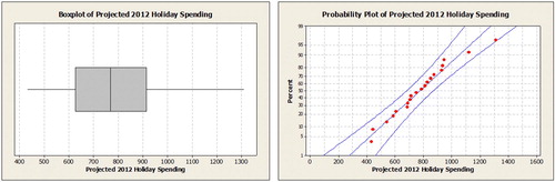
Table A.1 Optional problems to practice aspects of hypothesis testing.

Challenging aspect	Optional extra practice
A. Writing the hypotheses	Section 10.1 # 15–21
B. Deciding whether a particular test (like 1-PropZTest) is appropriate	Section 10.2 Ex. 1, 2, 4
C. Finding the p-value	Section 10.2 # 7–11
D. Interpreting the results	Section 10.1 # 23–33
E. Some other part

Table A.2 Descriptive statistics: projected spending.

Variable	N	Mean	SD	Minimum	Q1	Median	Q3	Maximum
Projected	20	776.9	214.6	430.9	625.9	767.8	914.2	1310.0
spending

Appendix B

Sample Lesson Plans

Below are the lesson plans that were used to teach the topics from chapter 10 that were part of this study: the 1-proportion Z-test (taught by worked examples) and the 1-sample t-test (taught by practice problems). Where appropriate, the correct answers of interpretation questions and practice problems are indicated in italics or bold.

Chapter 10 Worked Examples: 1-Proportion Z-Test

Mini-Lecture

A p-value is the probability of observing a sample result as extreme as, or more extreme than, what we observed, assuming that the null hypothesis is true. In other words, it’s the probability of getting a result at least as extreme as what we got, simply due to sampling variation (random differences in the sample we chose).

If p-value is “small” (less than significance level $\alpha )$, then we consider the study to be strong evidence against the null hypothesis.

To test $H_0:p=p_0$:

• Check that $n{p}_0\left(1-p_0\right)\ge 10$.

• Check that $n\le .05N$, where n is the sample size and N is the population size.

• If both of these conditions are true, then use Stat → Tests → 1-Prop ZTest on a TI-83 or TI-84 calculator.

Lecture Example

In 2001, 38% of families ate dinner together every night. A sociologist wants to know if this proportion has decreased.

So, the hypotheses we want to test are$$\begin{array}{c}{H}_0:p=0.38\\ H_a:p<0.38\end{array}$$where p is the proportion of all families who eat dinner together every night now.

The sociologist samples 1122 families and finds 403 who eat dinner together every night (Sullivan 2013, p. 493). Let’s check the conditions for a 1-proportion Z-test:

• • $n{p}_0\left(1-p_0\right)=1122\times 0.38\times 0.62=264.34\ge 10$

• $20n=20\times 1122 = 22,440.$ This is less than the number of families in US, so $1122\le 0.05N$.

The conditions are satisfied, so we can use Stat → Tests → 1-Prop ZTest on a calculator.

Ask students to try using their calculators to compute a p-value. Guide them through selecting the appropriate arguments for the function:$$p_0=0.38,x=403,n=1122, \text{prop}<p_0$$

Ask students what p-value they got. The answer should be 0.07539.

Conclusion: At the α = 0.05 level of significance, there is not enough evidence to claim that the proportion of all families who eat dinner together every night has decreased.

Experimental Phase

Have students read Worked Example 1, parts a and b.

Worked Example 1

1a. A carnival worker claims to be able to tell people’s birth months by psychic powers, more accurately than if he were just guessing. Write the null and alternative hypotheses to test this claim.

There are 12 months in the year, so if the carnival worker guesses at random, we expect that he will be right about $\frac{1}{12}$ of the time. So the null hypothesis is$$H_0:p=\frac{1}{12},$$where p is the proportion of birth months that the carnival worker would get right, if he attempted to tell the birth months of every person in the population.

(Note that this scenario is asking about a proportion of birth months that he gets right, so the parameter should be p, not μ.)

We want to test the carnival worker’s claim that he gets more right than if he were guessing. So, we should use the alternative hypothesis$$H_a:p>\frac{1}{12}$$making this a 1-sided test.

b. Out of 80 people at the fair, the carnival worker successfully guesses 9 people’s birth months (Sullivan 2013, p. 493). Is it appropriate to use 1-prop ZTest to test the claim?

80 × 20 = 1600, which is less than the population size of the US. So, the sample size is less than 5% of the population size. That means we can treat the observations as being independent.

In this hypothesis test, the sample size is $n =$80. The hypothesized proportion is $p_0=\frac{1}{12}.$ So$$n{p}_0\left(1-p_0\right)=80\times \frac{1}{12}\times \left(\frac{11}{12}\right)=6.1111$$

6.1111 is less than 10, so a normal distribution will not be a good approximation for $\widehat{p}$ This means that it is not appropriate to use 1-prop ZTest to test the claim.

When $n{p}_0\left(1-p_0\right)<10$, you have two good options:

• Gather a larger sample, or

• Do the hypothesis test in Minitab, which can use a binomial distribution to compute the exact p-value.

When students have finished reading, ask Interpretation Questions 1 and 2 to check understanding. (I had students input answers to all interpretation questions using iClickers.)

Interpretation Question 1

What is the parameter in this example?

1. The proportion of birth months the carnival worker got right, out of the 80 people at the fair.

2. The proportion of birth months the carnival worker would get right, if he attempted to tell the birth months of every person in the population.

3. The average number of birth months the carnival worker would get right, if he attempted to tell the birth months of every person in the population.

Interpretation Question 2

What should you do when$$n{p}_0\left(1-p_0\right)<10?$$

1. Gather a larger sample

2. Do the hypothesis test in Minitab

3. Panic!

4. Either A or B

Reveal correct answers and discuss briefly, based on how many students answered incorrectly. Then have students read Worked Example 2, part a.

Worked Example 2, part a

2. According to OSHA, 75% of restaurant employees say that work stress has a negative impact on their personal lives. You want to know if the proportion is different for people who work in university cafeterias, so you survey 100 people. 68% of the people you survey say that work stress has a negative impact on their personal lives.

a. Write the null and alternative hypotheses for this test.

In this problem, we’re interested in a percentage or a proportion, not a mean, so the parameter should be p. The null hypothesis should be that p equals some established value—not the value from the sample. So, the null hypothesis is$$H_0:p=0.75,$$where p is the proportion of people in the population of all university cafeteria workers who say that work stress has a negative impact on their personal lives.

(Notice that p isn’t the proportion of all restaurant workers. That’s because we already know that 75% of the population of restaurant workers have too much work stress. The goal of the hypothesis test is to find out whether cafeteria workers are different from this.)

Always write your alternative hypothesis before looking at the data. In this case, you should ignore the fact that 68% of the sample had too much work stress, and just look at the words, “You want to know if the proportion is different for people who work in university cafeterias.” That tells us that we would be equally interested to find that university cafeterias are more stressful than restaurants as if they’re less stressful. In other words, we have no particular reason to expect the difference to be in one direction versus the other.

The words “different for” tell us that we want the alternative hypothesis$$H_0:p\ne 0.75,$$which gives a 2-sided test.

When students have finished reading, ask Interpretation Question 3 to check understanding.

Interpretation Question 3

Why is the null hypothesis $H_0:p=0.75$ instead of $H_0:p=0.68$?

1. 0.75 is larger than 0.68.

2. 0.75 is the value that appears first in the problem.

3. 0.75 is the established value; 0.68 is the value from the sample.

Reveal correct answers and discuss briefly, based on how many students answered incorrectly. Then have students read Worked Example 2, part b.

Worked Example 2, part b

b. Find the p-value for this test.

In this sample, it is appropriate to use 1-prop ZTest to find the p-value. (You can check this yourself.) Before we do so, we need to find x, the number of “successes” (people who said yes) in our sample. We know that our sample size was $n =$100 people, and the sample proportion of people who said yes was $\widehat{p}=0.68$. So to find x, we use$$x=n\widehat{p}=100\times 0.68=68$$

Now we can use Stat → Tests → 1-prop ZTest with $p_0=0.75$ (the value in the null hypothesis), $x =$68, $n =$100, prop $\ne p_0$ (the alternative hypothesis).

This gives a p-value of 0.10597.

When students have finished reading, ask Interpretation Question 4 to check understanding.

Interpretation Question 4

How can you find x when it’s not given in the problem?$$\begin{array}{c}\mathit{x\; =\; n}\widehat{\mathit{p}}\\ x=\mathit{np}\\ x=\frac{\widehat{p}}{n}\\ x=\frac{p}{n}\end{array}$$

Reveal correct answers and discuss briefly, based on how many students answered incorrectly. Then have students read Worked Example 2, part c.

Worked Example 2, part c

c. Using α = 0.05, write the conclusion in the context of the problem.$$0.10597>0.05$$

Our p-value is larger than the level of significance, so we should retain H₀. In the context of the problem, our conclusion is that there is not enough evidence to claim that the proportion of all cafeteria workers who are negatively affected by work stress is different from 0.75.

When students have finished reading, ask Interpretation Question 5 to encourage self-reflection on the learning process and provide targeted resources for additional practice outside of class.

Interpretation Question 5

In your opinion, what is the most challenging part of hypothesis testing?

(Allow students to choose from Table A.1; then display options for extra practice on different topics.)

Chapter 10 Practice Problems: 1-Sample T-Test

Mini-lecture/Lecture example

The average volume of the hippocampus (the part of the brain responsible for long-term memory storage) in teenagers is 9.02 cm³. Researchers wanted to know whether the average size is lower among teenagers who are alcoholic.

So, the hypotheses we want to test are$$\begin{array}{c}{H}_0:\mu =9.02,\\ H_a:\mu <9.02,\end{array}$$where μ is the mean volume of the hippocampus in all teenagers who are alcoholic.

The researchers tested 12 alcoholic teenagers and found that hippocampus sizes were approximately normally distributed, with $\overline{x}=8.10{\text{cm}}^3$ and s = 0.7 (Sullivan 2013, p. 503).

A t-test is a hypothesis test for testing $H_0:\mu ={\mu }_0$. For this test to be appropriate, we need $\overline{x}$ to be normally distributed. This means that either the population should be approximately normal, or the sample size should be at least 30.

To conduct a t-test on a TI-83 or TI-84, use Stat → Tests → T-Test. Select Stats.

Ask students to try using their calculators to compute a p-value for the lecture example. Guide them through selecting the appropriate arguments for the function:$${\mu }_0=9.02,\overline{x}=8.2,s_x=0.7,n=12,\mu <{\mu }_0.$$

Ask students what p-value they got. The answer should be $4.1315\times {10}^{-4}$.

Conclusion: At the $\alpha =0.01$ level of significance, there is enough evidence to claim that the mean size of the hippocampus in all alcoholic teenagers is less than 9.02 cm³.

Experimental Phase

Have students solve Practice Problems 1–3 and submit answers via iClickers. After each problem, explain briefly and/or allow students time to discuss answers with classmates, depending on how many students answered incorrectly.

Practice Problem 1

In 2008, the mean travel time to work in Collin County, Texas, was 27.3 min. The Department of Transportation reprogramed the traffic lights to try to reduce travel time (Sullivan 2013, p. 501). The DoT wants to know if they have been successful. What hypotheses should we use?$$\begin{array}{c}A.H_0:\mu =27.3;H_a:\mu \ne 27.3\\ B.{\mathit{H}}_0:\mathit{\mu }=27.3;{\mathit{H}}_a:\mu <27.3\\ C.H_0:\mu =27.3;H_a:\mu >27.3\end{array}$$

Practice Problem 2

In a random sample of 2500 commuters, $\overline{x}=27.0$ min and s = 8.5 (Sullivan 2013, p. 501). Find the p-value.

A. .03887

B. .05443

C. .07774

Practice Problem 3

What is your conclusion at the α = 0.05 level?

1. There is enough evidence to claim that the mean commute time is less than 27.3 min.

2. There is not enough evidence to claim that the mean commute time is less than 27.3 min.

Mini-lecture

If you were a commuter in this county, would you be happy about the difference between 27.3 min and 27.0 min? Probably not. This is an example of a difference that’s statistically significant but not practically important. Statistical significance can happen when the difference between $\overline{x}$ and μ₀ (or between $\widehat{p}$ and p₀) is large (in terms of standard deviations), or when the sample size is very large.

Experimental Phase

Have students solve Practice Problems 4–6. Students will submit answers to problems 4–5 via iClickers. After each problem, explain briefly and/or allow students time to discuss answers with classmates, depending on how many students answered incorrectly.

Practice Problem 4

The average credit score is 703.5. A financial advisor wondered whether people making more than $100,000 per year have higher credit scores, on average (Sullivan 2013, p. 504). The financial advisor sampled 40 high-income individuals and found the [simulated] results in Figure A.1 (Minitab 2010).

Is a t-test appropriate?

1. Yes

2. No

Practice Problem 5

We are testing$$\begin{array}{c}{H}_0:\mu =703.5\\ H_a:\mu >703.5\end{array}$$

Out of 40 high-income individuals, the sample mean credit score was 714.2, with a standard deviation of 83.2 (Sullivan 2013, p 504). Find the p-value.

A. 2080

B. .2105

C. .2816

D. .4209

Practice Problem 6

In your notebook, write the conclusion in the context of the problem, using α = 0.05. (Give students time to write, then ask them to compare answers with those sitting near them.)

Answer: There is not enough evidence to claim that the mean credit score is higher than 703.5 in the population of high-income individuals.

Appendix C:

Sample Assessment Questions

The exam questions used to assess student understanding of the topics from chapter 10 are included below.

Assessment for Chapter 10: 1-Sample Z-test of Proportions

Exam 3

According to the Centers for Disease Control, in 2008, 18% of adult Americans smoked cigarettes. In 2013, a survey of 199 randomly selected adult Americans found 18 people who smoked cigarettes (Sullivan 2013, p. 494). Does this constitute evidence that the proportion of adult Americans who smoke has changed? Use a 1-sample Z-test of proportions.

1. State the null and alternative hypotheses. Use the most appropriate symbol ($\mu ,x″)$ and write in words what it represents. [5 points; scores of 4.5 or 5 were counted as “essentially correct.”]

2. Find the p-value. [2 points; a score of 2 was counted as “essentially correct.”]

3. State your conclusion in the context of the problem. Use α = 0.05. [5 points; a score of 5 was counted as “essentially correct.”]

Final Exam

An existing medication for acid reflux is known to heal the esophagus of 94% of patients within 8 weeks (Sullivan 2013, p. 493). A pharmaceutical company has just developed a new medication for acid reflux, and they want to know if it is better than the existing medication.

1. State the null and alternative hypotheses for a 1-Sample Z-test of a Proportion. Use the most appropriate symbol ($\mu ,\overline{x},p$, or) and write in words what it represents. [5 points; scores of 4.5 or 5 were counted as “essentially correct.”]

2. The pharmaceutical company administers their medication to a random sample of 224 patients with acid reflux. The medication works to heal the esophagus of 213 patients within 8 weeks (Sullivan 2013, p. 493). Find the p-value. [2 points; a score of 2 was counted as “essentially correct.”]

3. State your conclusion in the context of the problem. Use α = 0.05. [5 points; a score of 5 was counted as “essentially correct.”]

Assessment for Chapter 10: 1 Sample T-Test

Exam 3

The mean FICO credit score in the U.S. is 703.5. A credit analyst wondered whether the mean credit score of people in Wisconsin is different from the national average.

1. State the null and alternative hypotheses. Use the most appropriate symbol ($\mu ,\overline{x},p$, or) and write in words what it represents. [5 points; scores of 4.5 or 5 were counted as “essentially correct.”]

   The Minitab output in Figure A.2 (Minitab 2010) shows the results of the credit analyst’s investigation.

2. Find the p-value. [2 points; a score of 2 was counted as “essentially correct.”]

3. State your conclusion in the context of the problem. Use a 0.05 level of significance. [5 points; a score of 5 was counted as “essentially correct.”]

Final Exam (Multiple choice; only the correct answer was counted as “essentially correct.”)

According to the American Research Group, the average amount spent per household on holiday gifts was $850 in 2007. A researcher believes that average has declined. To assess this claim, the researcher obtains a simple random sample of 20 households and determines the projected holiday spending. The results are shown in Figure A.3 and Table A.2 (Minitab 2010).

Determine the result of the appropriate hypothesis test.

1. Do not reject H₀ at the 10% level of significance.

2. Reject H₀ at the 10% level of significance, but not at the 5% level of significance.

3. Reject H₀ at the 5% level of significance, but not at the 2.5% level of significance.

4. Reject H₀ at the 2.5% level of significance, but not at the 1% level of significance.

5. Reject H₀ at the 1% level of significance.

References

- American Statistical Association (2016), “Guidelines for Assessment and Instruction in Statistics Education (GAISE) College Report,” available at http://www.amstat.org/asa/files/pdfs/GAISE/GaiseCollege_Full.pdf.
- Ancker, J. S. (2006), “The Language of Conditional Probability,” Journal of Statistics Education, 14. DOI:10.1080/10691898.2006.11910584.
- Atkinson, R. K., Derry, S. J., Renkl, A., and Wortham, D. (2000), “Learning From Examples: Instructional Principles From the Worked Examples Research,” Review of Educational Research, 70, 181–214. DOI:10.3102/00346543070002181.
- Atkinson, R. K., and Renkl, A. (2007), “Interactive Example-Based Learning Environments: Using Interactive Elements to Encourage Effective Processing of Worked Examples,” Educational Psychology Review, 19, 375–386. DOI:10.1007/s10648-007-9055-2.
- Atkinson, R. K., Renkl, A., and Merrill, M. M. (2003), “Transitioning From Studying Examples to Solving Problems: Effects of Self-Explanation Prompts and Fading Worked-Out Steps,” Journal of Educational Psychology, 95, 774–783. DOI:10.1037/0022-0663.95.4.774.
- August, L. O., Hurtado, S. Y., Wimsatt, L. A., and Dey, E. L. (2002), “Learning Styles: Student Preferences vs. Faculty Perceptions,” in 42nd Annual Forum for the Association for Institutional Research, Toronto, available at http://web.stanford.edu/group/ncpi/unspecified/student_assess_toolkit/pdf/learningstyles.pdf.
- Berry, T., Cook, L., Hill, N., and Stevens, K. (2010), “An Exploratory Analysis of Textbook Usage and Study Habits: Misperceptions and Barriers to Success,” College Teaching, 59, 31–39. DOI:10.1080/87567555.2010.509376.
- Carlson, K. A., and Winquist, J. R. (2011), “Evaluating an Active Learning Approach to Teaching Introductory Statistics: A Classroom Workbook Approach,” Journal of Statistics Education, 19. DOI:10.1080/10691898.2011.11889596.
- Clump, M. A., Bauer, H., and Bradley, C. (2004), “The Extent to Which Psychology Students Read Textbooks: A Multiple Class Analysis of Reading Across the Psychology Curriculum,” Journal of Instructional Psychology, 31, 227–232.
- Dexter, F., Masursky, D., Wachtel, R. E., and Nussmeier, N. A. (2010), “Application of an Online Reference for Reviewing Basic Statistical Principles of Operating Room Management,” Journal of Statistics Education, 18. DOI:10.1080/10691898.2010.11889588.
- Gage, M., Pizer, A., and Roth, V. (2002), “WeBWorK: Generating, Delivering, and Checking Math Homework via the Internet,” in Proceedings of the 2nd International Conference on the Teaching of Mathematics.
- Gelman, A., Carlin, J. B., Stern, H. S., and Rubin, D. B. (2004), Bayesian Data Analysis (2nd ed.), Boca Raton, FL: Chapman & Hall/CRC.
- Giraud, G. (1997), “Cooperative Learning and Statistics Instruction,” Journal of Statistics Education, 5. DOI:10.1080/10691898.1997.11910598.
- Haapalainen, E., Kim, S. J., Forlizzi, J. F., and Dey, A. K. (2010), “Psycho-Physiological Measures for Assessing Cognitive Load,” in Proceedings of the 12th ACM International Conference on Ubiquitous Computing.
- Kalyuga, S., Chandler, P., Tuovinen, J., and Sweller, J. (2001), “When Problem Solving Is Superior to Studying Worked Examples,” Journal of Educational Psychology, 93, 579–588. DOI:10.1037/0022-0663.93.3.579.
- Keeler, C., and Steinhorst, K. (2001), “A New Approach to Learning Probability in the First Statistics Course,” Journal of Statistics Education, 9. Available at http://jse.amstat.org/v9n3/keeler.html.
- Layne, B. H., and Huck, S. W. (1981), “The Usefulness of Computational Examples in Statistics Courses,” Journal of General Psychology, 104, 283–285. DOI:10.1080/00221309.1981.9921046.
- Lunn, D. J., Thomas, A., Best, N., and Spiegelhalter, D. (2000), “WinBUGS—A Bayesian Modelling Framework: Concepts, Structure, and Extensibility,” Statistics and Computing, 10, 325–337. DOI:10.1023/A:1008929526011.
- Magalhães, M. N., and Magalhães, M. C. C. (2014), “A Critical Understanding and Transformation of an Introductory Statistics Course,” Statistics Education Research Journal, 13, 28–41.
- Minitab (2010), Minitab 17 Statistical Software [Computer Software], State College, PA: Minitab, Inc.
- Paas, F. G. W. C. (1992), “Training Strategies for Attaining Transfer of Problem-Solving Skill in Statistics: A Cognitive-Load Approach,” Journal of Educational Psychology, 84, 429–434. DOI:10.1037/0022-0663.84.4.429.
- Paas, F. G. W. C., and Van Merriënboer, J. J. G. (1994), “Variability of Worked Examples and Transfer of Geometrical Problem-Solving Skills: A Cognitive-Load Approach,” Journal of Educational Psychology, 86, 122–133. DOI:10.1037/0022-0663.86.1.122.
- Quilici, J. L., and Mayer, R. E. (1996), “Role of Examples in How Students Learn to Categorize Statistics Word Problems,” Journal of Educational Psychology, 88, 144–161. DOI:10.1037/0022-0663.88.1.144.
- R Core Team (2015–2017), R: A Language and Environment for Statistical Computing, Vienna, Austria: R Foundation for Statistical Computing, available at https://www.R-project.org/.
- Renkl, A., and Atkinson, R. K. (2003), “Structuring the Transition From Example Study to Problem Solving in Cognitive Skill Acquisition: A Cognitive Load Perspective,” Educational Psychologist, 38, 15–22. DOI:10.1207/S15326985EP3801_3.
- Renkl, A., Atkinson, R. K., Maier, U. H., and Staley, R. (2002), “From Example Study to Problem Solving: Smooth Transitions Help Learning,” Journal of Experimental Education, 70, 293–315. DOI:10.1080/00220970209599510.
- Rinaman, W. C. (1998), “Revising a Basic Statistics Course,” Journal of Statistics Education, 6. DOI:10.1080/10691898.1998.11910613.
- Ringenberg, M. A., and VanLehn, K. (2006), “Scaffolding Problem Solving With Annotated, Worked-Out Examples to Promote Deep Learning,” in Intelligent Tutoring Systems, Berlin, Heidelberg: Springer, pp. 625–634.
- Rohrer, D. (2009), “The Effects of Spacing and Mixing Practice Problems,” Journal for Research in Mathematics Education, 40, 4–17.
- Rossman, A. J., and Short, T. H. (1995), “Conditional Probability and Education Reform: Are They Compatible?,” Journal of Statistics Education, 3. DOI:10.1080/10691898.1995.11910486.
- Salden, R. J. C., Aleven, V. A. W. M. M., Renkl, A., and Schwonke, R. (2009), “Worked Examples and Tutored Problem Solving: Redundant or Synergistic Forms of Support?,” Topics in Cognitive Science, 1, 203–213. DOI:10.1111/j.1756-8765.2008.01011.x.
- Shernoff, D. J., Csikszentmihalyi, M., Shneider, B., and Shernoff, E. S. (2003), “Student Engagement in High School Classrooms From the Perspective of Flow Theory,” School Psychology Quarterly, 18, 158–176. DOI:10.1521/scpq.18.2.158.21860.
- Sullivan, M. (2013), Statistics: Informed Decisions Using Data (4th ed.), Boston, MA: Pearson.
- Tarmizi, R. A., and Sweller, J. (1988), “Guidance During Mathematical Problem Solving,” Journal of Educational Psychology, 80, 424–436. DOI:10.1037/0022-0663.80.4.424.
- Titman, A. C., and Lancaster, G. A. (2011), “Personal Response Systems for Teaching Postgraduate Statistics to Small Groups,” Journal of Statistics Education, 19. DOI:10.1080/10691898.2011.11889614.
- van Gog, T., and Kester, L. (2012), “A Test of the Testing Effect: Acquiring Problem-Solving Skills From Worked Examples,” Cognitive Science, 36, 1532–1541.
- Vaughn, B. K. (2009), “An Empirical Consideration of a Balanced Amalcamation of Learning Strategies in Graduate Introductory Statistics Classes,” Statistics Education Research Journal, 8, 106–130.
- Winquist, J. R., and Carlson, K. A. (2014), “Flipped Statistics Class Results: Better Performance Than Lecture Over One Year Later,” Journal of Statistics Education, 22. DOI:10.1080/10691898.2014.11889717.
- Zetterqvist, L. (1997), “Statistics for Chemistry Students: How to Make a Statistics Course Useful by Focusing on Applications,” Journal of Statistics Education, 5. DOI:10.1080/10691898.1997.11910525.