Questionable Claims for Simple Versions of the Bootstrap

Abstract

Recent years have seen increasing interest in incorporating resampling methods into introductory statistics courses and the high school mathematics curriculum. While the use of permutation tests for data from experiments is a step forward, the use of simple bootstrap methods for sampling situations is more problematical. This article demonstrates via counterexamples that many of the claims made for these simple methods are simply wrong. Their use with beginners can only be justified after their true properties have been fully researched, and their many limitations explained to students. Supplementary materials for this article are available online.

KEYWORDS:

• Bootstrap
• Common Core
• Confidence interval
• Resampling
• Robust
• Simulation

1 Introduction

No doubt you remember doing confidence intervals for a mean using the normal distribution or Student’s t distribution. “The” bootstrap is an alternative method that is used for means and many other statistics as well. There are quotation marks surrounding the first word of the last sentence because there are many versions of the bootstrap. This article discusses the two simple versions that are likely to appear in an introductory statistics course in college, or as an implementation of the Common Core (Common Core State Standards Initiative, n.d.) in high schools. For example, a bootstrap simulation could be interpreted as one way to meet Common Core Standard HSS.IC.8.4.

CCSS.Math.Content.HSS.IC.B.4 Use data from a sample survey to estimate a population mean or proportion; develop a margin of error through the use of simulation models for random sampling.

Two general kinds of claims are made for these methods: that they have pedagogical advantages over the traditional methods, and that they work “better” in some ways than do the traditional methods. This article will concentrate on the latter claims and show that most of those are untrue. Some of the pedagogical claims will be treated in passing. It is important to note that matters are very different for more advanced versions of the bootstrap. (Two such are discussed in Hesterberg et al. (2007), pp. 45–48.) Those work much better (in the sense of offering actual coverage close to nominal), but are too complicated to explain to beginners, and hence, lose many of their pedagogical advantages. It would be nice at this point to cite journal articles expressing these claims, but such claims are more rumor or folklore, and do not usually appear in research journals. Tracing their origin and spread would be more a matter for sociological or historical research and is not attempted here. We will note in passing that such claims are often implicit. A textbook may list conditions under which t-tests can be used, but not mention any comparable conditions for bootstrapping, thereby suggesting there are none. Or a writer may suggest using “the” bootstrap when assumptions for t fail, without specifying which bootstrap method might be appropriate or whether the conditions for that method have been satisfied.

Because some readers may not be familiar with any form of the bootstrap, it might be wise to briefly explain the two simple versions commonly seen by beginners, and contrast them with traditional methods. All these methods are used in situations where we have a simple random sample from a population and wish to use it to estimate a population parameter. We will use the t-interval for a single mean as an example. In general, we wish to estimate a population parameter (the population mean in this case) and use some sample statistic (here the sample mean) to estimate it. (While using the corresponding sample statistic to estimate the population parameter is common with traditional methods, and the norm for the bootstrap, it is not the only choice, nor is it always a good choice, see, e.g., Bullard, 2007 on the German Tank Problem.)

Next we want some measure of how far off that estimate might be. For traditional methods, that is often a standard error—the standard deviation of the sampling distribution of our estimator, computed from a formula based on theory. Then we can say something like, “The population mean is probably within one standard error of the sample mean.” Finally, we make “probably” a little more precise. This requires knowing the shape of the sampling distribution. Theory tells us that it is approximately normal (for large samples from “nice” populations), but to allow for the fact that we also estimated the standard error from sample data we need to use an adjusted normal distribution known as “Student’s t.” This is the traditional approach for means.

The bootstrap almost always estimates a population parameter with the corresponding sample statistic, but it estimates the variability and shape of the sampling distribution with a computer simulation. As always, it is not practical to take many more samples from the population, so what we do is sample with replacement from the sample we have. We want samples of the same size as the original one, because we expect the answer depends on sample size. So we do what amounts to putting the original sample in a hat and drawing items one at a time, recording the result, putting the item back in the hat, and drawing again. By this method, we eventually get a bootstrap sample the same size as the original. Then we draw another such sample and another. When we have a large number of these bootstrap samples, we look at the distribution of the means (in this case) of the many bootstrap samples, and use that to estimate the variability and shape of the real sampling distribution.

The first bootstrap method we will look at is the percentile bootstrap which estimates the ends of a 95% confidence interval for the mean with the 2.5th and 97.5th percentiles of the bootstrap distribution, thus tacitly assuming these are good estimators of the corresponding percentiles of the sampling distribution. This is directly analogous to using those same percentiles of the t-distribution as we do with a t-interval. This is the classic basic bootstrap. An example of a recent public appearance of this method to high school students would be Free Response question 6 on the 2019 AP Statistics exam (College Board, 2019).

The other simple method, often used in Common Core curricula, instead finds the standard deviation of the bootstrap distribution, uses that as an estimate of the standard error of the sampling distribution, and then uses the sample mean plus or minus twice that estimate (called “margin of error”) for a 95% confidence interval, implicitly relying on the assumption that the bootstrap distribution is normal as well as the “empirical rule” for normal distributions. Thus, the bootstrap standard deviation replaces a standard error computed from a formula, and “2” replaces z = 1.96 or a value of t from a table. An example of a recent public appearance of this method to high school students would be item 35 on the January 2019 New York State Regents (2019) Exam for Algebra II. To save space in the already crowded tables that follow, we will denote using this bootstrap estimate of the standard error and its associated intervals as “2SE.”

A number of claims have been rumored for these bootstrap intervals.

1. They are more accurate than traditional methods for small samples.

2. They are more accurate when the population is not normally distributed.

3. They work for any statistic, not just means.

4. They make fewer or no assumptions.

5. They are easier for students to understand.

Items 1–3 could be seen as special cases of 4, so let’s note first that the bootstrap methods described above do make assumptions about what is a good estimator of what. In particular, they assume that the bootstrap distribution is a good estimator of the sampling distribution.

In an effort to check these claims, bootstrap methods could be evaluated on two grounds. One would be a theoretical justification comparable to those appealing to the central limit theorem for traditional methods. Popularizers of the bootstrap generally assume that the method is “intuitively obvious” and give no such justification. Statistical researchers have generally found the simple versions of the bootstrap wanting, and moved on to more complex versions. Their negative conclusions are often based on the other ground—simulation studies. For those, we create a specific population on a computer, take a large number of samples, compute a confidence interval by the method under study for each sample, and then check to see if 95% of such “95%” confidence intervals do in fact include the population parameter. Because we probably did not include every possible sample, this will give only an approximation to the percent actually including the population value, but we can increase accuracy by taking more samples, and estimate the size of this error with traditional methods for estimating proportions.

2 Estimating Means With Small Samples

Diez (n.d.) has done such simulation studies and made them available online. His work is limited to estimating means. He looked at sample sizes of 5, 10, and 30, and took samples from a normal distribution and four skewed distributions ranging from moderately to very skewed. Since the conditions for the t-interval are very close to satisfied when sampling from a normal distribution, the coverage (percent actually including the population value) in that case was very close to 95% for the t-intervals. The coverage in the same case for the two bootstrap methods discussed here are around 90% for a sample size of 10 and around 84% for samples of size 5. Neither is an acceptable level of accuracy. In fact, Diez also looked at the traditional “large sample” test using z and that performed better than either bootstrap method for both of these small sample sizes. It would be hard to find an introductory statistics textbook that considered using large sample methods appropriate here, and logical consistency would suggest that the inferior accuracy of these bootstrap methods would have to be considered inappropriate as well.

But that assumes that the work of Diez is correct. The first step in our study was to try to replicate his results. To do this, we coded our simulations from scratch and have not seen the code used by Diez. In addition, we tried to make the code as simple as possible to facilitate checking it. The code for our first example is in the R script coverageNorm2se.R. Unless otherwise stated, the number of trials and resamples is 1000 for all the simulations reported here. As a result the last digit in the observed coverage is doubtful. This choice of this modest number of repetitions was based on a number of considerations. Our goal here was to look for counterexamples. Initial tests with 10,000 repetitions took a while to run, and offered no useful increase in accuracy. With Diez reporting 84% coverage for nominal 95% intervals, there seemed to be no need to see if that 84% was really 83.7 or even 85.3—all these values would serve equally well as counterexamples. Then we anticipated that our brute force code might run slowly, and finally we preferred to use our time to seek further counterexamples rather than to refine the exact amount by which the method failed.

Table 1 shows sample results for the mean for the bootstrap method for the case that makes the interval the estimate plus or minus twice the bootstrap standard deviation. (We added samples sizes of 100 and 300 to those considered by Diez to get a better idea of how large a sample was required to get coverage near the nominal 95%.)

Table 1 Coverage of nominal 95% confidence intervals for for the mean for samples from a normal distribution, using ± twice the bootstrap standard deviation.

n	Coverage
5	84.7%
10	89.3%
30	93.4%
100	96.2%
300	94.8%

These results are consistent with those of Diez for the two smaller sample sizes he examined. That gave us confidence in his results and in our own code. (Additional testing not reported here gave similar results.) Note that using traditional t-intervals in this situation gives true 95% coverage for all these sample sizes. The conclusion is, at least for means of small samples from a normal distribution, that this simple bootstrap method does not offer any advantage, and does not offer adequate coverage accuracy for small samples.

3 Estimating Means With Small Samples From Skewed Populations

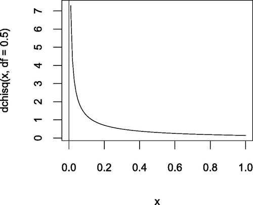
But what if the population is not normal? For the most skewed of the distributions Diez considered, a chi-squared distribution with 0.5 degrees of freedom (represented in Figure 1), Diez found that the coverage for t-intervals dropped to 74% and 80% for sample sizes of 5 and 10, respectively. Not so good, but coverage for both the simple bootstrap intervals dropped to around 66% and 77%—even worse, though none of the methods gave acceptable accuracy. The conclusion is that these simple methods are not a good remedy for skewness with these small sample sizes. At this point, we considered the work of Diez on skewed continuous populations to be essentially correct and we moved on to other cases.

Fig. 1 Chi-squared distribution with 0.5 degrees of freedom.

4 Other Populations

The purpose of this research project was to extend the results of Diez in a number of directions. In Table 1, there are some results for larger sample sizes. The next extension we will consider is estimating means of some other populations. Of course, we cannot consider every possible population, but we have selected several that seemed to be of special interest. One was the symmetric but quite heavy-tailed distribution of Student’s t with three degrees of freedom. (We skipped one or two degrees of freedom as downright pathological.) This was contrasted with a nearly normal t distribution with 1000 degrees of freedom. Next, it seemed that theoretical distributions extending to infinity might be questioned on the ground that no real data do so. Hence, we looked at a population consisting of the integers from 1 to 1000, Finally we looked at two populations with just two values, 0 and 1—distributions with no tails at all.

Table 2 gives the results for both simple bootstrap methods when sampling from a population following the t-distribution with three degrees of freedom and five different sample sizes. Our code is in the R scripts coverageT.R and coverageT2se.R. Each percentile bootstrap interval was created from 1000 resamples from a single original sample. Then a new sample was taken from the population and a new interval created. This process was repeated for a total of 1000 trials/intervals.

Table 2 Coverage of nominal 95% confidence intervals for the mean using simple bootstrap methods when sampling from a t-distribution with three degrees of freedom.

df	n	Trials	Resamples	Level	Percentile	2SE
3	5	1000	1000	95%	84.7%	87.0%
3	10	1000	1000	95%	90.4%	91.1%
3	30	1000	1000	95%	91.9%	94.7%
3	100	1000	1000	95%	93.7%	94.2%
3	300	1000	1000	95%	95.0%	94.6%

These results are roughly comparable to the results of Diez for the percentile bootstrap on samples from a normal distribution, and give better coverage than the results he obtained for skewed distributions. Whether they are good enough is a matter of opinion. There are no universally agreed upon standards for how close to nominal the coverage should be. Hesterberg (2014) has offered some fairly strict standards. The following more lenient approach is used here. The most common levels in practice are 90, 95, and 99%, so here we will use the standard that a 95% nominal interval should have coverage that is closer to 95% than it is to 90 or 99%. By that standard we get adequate coverage accuracy in these cases only for sample sizes of 100 or more with the percentile bootstrap, 30 or more for the bootstrap based on the standard deviation.

Diez examined five populations: a normal distribution and four chi-squared distributions with varying degrees of freedom (5, 3, 1, 0.5) and hence skewness. For the populations and three samples sizes (5, 10, 30) considered by Diez, accuracy acceptable by our standards was obtained only for samples of size 30 from a normal or mildly skewed population. Table 2 suggests the simple bootstrap methods give acceptable accuracy with a heavy-tailed distribution if we use larger samples than Diez considered. So the advocates of the percentile bootstrap are right that the method works (at least sometimes), but mistaken that it is particularly suited to small samples.

A disadvantage of simulation studies is that there is no end to the different combinations of population, sample size, bootstrap method, etc. that one might consider. This article presents a convenience sample of cases sufficient to establish that a great deal more work on the properties of these methods is needed before presenting them to beginners.

Next we take a short side trip to examine the effect of varying the nominal coverage level of our intervals. In Table 3, the population is as above but we did 90 and 99% intervals instead of 95%, and used only the percentile bootstrap (R script coverageT.R).

Table 3 Coverage of nominal 90% and 99% confidence intervals for the mean for the percentile bootstrap method when sampling from a t-distribution with three degrees of freedom.

df	n	Trials	Resamples	Coverage90%	Coverage99%
3	5	10,000	10,000	78.4	89.6
3	10	10,000	10,000	83.2	95.6
3	30	10,000	10,000	86.9	97.8
3	100	10,000	10,000	88.2	98.6
3	300	10,000	10,000	89.4	98.9

In the cases examined here, coverage is marginal for a sample size of 30, unacceptable for smaller samples, and good for sample sizes larger than 30. Of course, here as in all our simulations, we have to be cautious in extrapolating our results to sample sizes and population distributions not examined here. However, just as the work of Diez provided many counterexamples showing poor coverage for skewed populations, Table 3 provides plenty of examples of poor coverage for a symmetric but long-tailed distribution.

Returning to nominal 95% intervals, we looked at three symmetric distributions with shorter tails. The R function used for the simulations above has degrees of freedom as a parameter to allow investigating varying degrees of tail weight. That allowed drawing samples from a t distribution with 1000 degrees of freedom—the mythical “nearly normal” distribution so beloved of introductory textbooks (R script coverageT.R).

One possible objection to working with the theoretical distributions above and in the work of Diez is that they extend to infinity, while real populations do not. A bootstrap distribution is based on a single sample that is unlikely to contain the most extreme values of the population. This may cause the bootstrap distribution to poorly estimate the true sampling distribution by essentially cutting off its tails. This might be expected to be a bigger problem if said tails extend to infinity. This was addressed with a number of bounded populations. In Table 4, the population “1:1000” consists of the natural numbers from 1 to 1000. (R script coveragePD.R.) “t1000” is a population that follows a t-distribution with 1000 degrees of freedom. “N10k” is a population that consists of 10,000 random observations from a standard normal distribution. (Thus, it is a second “nearly normal” distribution, but bounded, as all samples were taken from the same 10,000 numbers.)

Table 4 Coverage of nominal 95% confidence intervals for for the mean for simple bootstrap methods when sampling from relatively “tame” distributions.

n	level	2SE cov:t1000	Percentile cov:t1000	Percentile cov:N10k	Percentile cov:1:1000
5	95%	84.8%	83.4%	84.6%	85.2%
10	95%	92.7%	91.3%	91.6%	91.3%
30	95%	94.2%	92.6%	93.5%	93.5%
100	95%	94.9%	93.9%	95.6%	94.6%

The results are not much different than the other 95% intervals discussed above or in the work of Diez. The pattern seems to be that the simple bootstraps give close to nominal coverage for large samples, often do so for samples of size 30, and do not do so for smaller samples.

Our final populations are two flavors of a population consisting entirely of 0’s and 1’s. If both values have probability 0.5, then we have a symmetric distribution with no tails. If the probability of a 1 is 0.9, we have a distribution that is not symmetric, but also has very short tails. By way of comparison, Table 5 includes coverage for both 0.5 and 0.9 for a classic method based on the normal distribution (N) as well as for both simple bootstrap methods. (R scripts coverageBern.R, coverageBern2se.R, and coverageBernZ1.R.)

Table 5 Coverage of nominal 95% confidence intervals for normal approximation (N) and two simple bootstrap methods when sampling from Binomial(n,p) distributions.

n	Level	Percentile:p = 0.5	2SD:p = 0.5	N:p = 0.5	Percentile:p = 0.9	2SE:p = 0.9	N:p = 0.9
5	95%	93.0%	92.5%	94.5%	39.6%	40.0%	42.2%
10	95%	88.8%	87.1%	89.4%	61.1%	65.9%	67.9%
30	95%	91.6%	94.9%	95.9%	78.6%	87.5%	79.5%
100	95%	94.3%	94.4%	94.4%	91.9%	92.7%	93.5%
300	95%	94.4%	96.0%	95.0%	93.1%	94.5%	93.8%

The most noteworthy aspect of the results for $p=0.5$ is that coverage does not increase smoothly with sample size. However, barring the fortuitous result for a sample of size 5, we see that all the methods work poorly for samples of size 10, with coverage improving for larger samples, as usual.

The most noteworthy aspect of the results for $p=0.9$ is that coverage for this simple distribution is worse than for any of the more exotic ones considered above or by Diez. The three methods do not give good accuracy here until the sample size reaches the hundreds.

For both 0.5 and 0.9 we do need to be careful in generalizing. Agresti and Coull (1998) showed that coverage is a discontinuous function of sample size. When we sample for proportions, the number of successes in the sample is always an integer. Thus, the bootstrap distribution is grainy, and we get step changes in coverage as we jump from one sample size to the next. In any case, our goal was to find counterexamples and the table provides many, along with little evidence of the bootstrap methods offering any advantage over the classical (and not very accurate) method based on the normal distribution. In fact, the bootstrap methods are nearly always inferior here. (See additional discussion in the next section.)

5 Other Statistics

It has been claimed that while t works only for means, these bootstrap methods work for many (even any) statistics. This claim was tested with simulation studies using a wide variety of common statistics. Earlier we took samples from a population of zeros and ones. If we think of these as representing failure and success, then the sample total will just be the number of successes and the sample proportion will just be the sample mean. So, though we might consider the sample proportion to be another statistic, it is actually a special case of the mean. (Indeed, if you look at a mathematical statistics book, you will find that the results for proportions are derived by applying the results for means to a 0–1 population.)

For these reasons, the results in Table 5 for 0–1 populations can be considered as investigations of using simple bootstrap methods with proportions. We can see in Table 5 that, when the population proportion is 0.5, the percentile bootstrap performs about as it does for other means from other populations, but, when the population proportion is 0.9, it performs even less well, needing sample sizes of around 300 to give reasonable coverage accuracy.

Confidence intervals for proportions are a difficult topic. Table 5 includes a method based on the Normal distribution. It is often called the “Wald interval” and is nearly universal in introductory statistics textbooks. However, there have long been doubts about its accuracy for small samples. Agresti and Coull (1998) investigated its inaccuracies in detail and found them to be greater than realized. We can see that in Table 5, where the Wald interval performs poorly—only marginally better than the percentile bootstrap. Agresti and Coull propose an adjusted interval that offers much better coverage yet is no more difficult for students to compute than the Wald interval, though we will not pursue that here. Instead, let us note that Agresti and Coull found that coverage was a very discontinuous function of population proportion and sample size. This can be seen in Table 5 where coverage when p = 0.5 is better for a sample size of 5 than of size 10 for both the percentile bootstrap and the Wald interval. A consequence is that we cannot be sure that the case illustrated in Table 5 is typical, and massive simulations, with large numbers of different sample sizes and population proportions, such as Agresti and Coull did, might be needed to fully evaluate the percentile bootstrap interval for proportions. At the moment, it seems doubtful that such would be worthwhile, especially considering that there is a simple method with much better coverage.

The claim that the bootstrap works for any statistic seems obviously false for statistics such as the population maximum. A percentile bootstrap interval would be based on resamples from a single sample. If that sample failed to include the population maximum, then all the maxima of bootstrap resamples would fall below the true value, and the 97.5th percentile could be expected to fall below many sample maxima. Hence, most of the intervals would not include the true value. To avoid situations such as we have with the normal distribution, where the population maximum, minimum, and range are undefined, simulations were done for a bounded population and a variety of common statistics all under the same conditions—95% percentile bootstrap intervals based on samples of size 30 from the integers from 1 to 1000. The results are in Table 6. (R script coveragePD.R)

Table 6 Coverage of nominal 95% confidence intervals for percentile bootstrap method when sampling 30 integers from 1 to 1000.

Parameter name	Parameter value	Coverage
50 percentile (median)	500.5	94.8%
75 percentile (Q3)	750.2	93.8%
90 percentile	900.1	86.7%
95 percentile	950.05	80.2%
99 percentile	990.01	25.5%
100 percentile (maximum)	1000	0.0%
Range	999	0.0%
IQR	499.4	95.8%
Variance	83,416.67	93.1%
SD	288.8194	93.2%
Coeff. of variation	0.5770618	93.8%

We see that even from this bounded and tailless distribution we get coverages of zero for statistics like the range or maximum. On the other hand we see that we get good coverage for several statistics (at least in this case). Matters are more complicated for percentiles. There are many different rules for computing percentiles. These simulations used the values provided by R, which are also given in the table. We see that while coverage is very good for the median (50 percentile) in this case (Hesterberg et al., 2007, pp. 18–36 seem to suggest we were just lucky.), coverage steadily deteriorates as we try to estimate more extreme percentiles.

Noting that coverage was good for the median with this symmetric distribution, simulations were run with other sizes of samples from the very skewed chi-squared distribution with 0.5 degrees of freedom. In this case they were nominally 90% intervals. The results are in Table 7 (R script coverageChi.R). Again we see surprisingly good results for samples of size 5, probably for reasons similar to our seeing the same effect for proportions.

Table 7 Coverage of nominal 90% confidence intervals for the median using percentile bootstrap method when sampling from a chi-squared distribution with 0.5 degrees of freedom.

n	Coverage
5	89.6%
10	86.8%
30	87.8%
100	89.5%

In any event, coverage for the median is adequate for all four sample sizes from this difficult situation, and similar results were obtained sampling from a normal distribution and one that followed the t-distribution with three degrees of freedom. This contrasts sharply with the results of Diez for estimating the mean using the same method. Coverage was inadequate for the sample sizes he tested: 5, 10, and 30. The results in Table 7 are the first case in which we have seen the percentile bootstrap perform well for small samples.

6 One-Sided Inference

Hesterberg (2014) has argued that all inference is essentially one-sided. At least one can say that very often the consequences of the truth landing on one or the other side of the null can be very different, and that a different choice of alpha might be appropriate for the two sides. All intervals that involve adding and subtracting a margin of error from an estimate assume a symmetric sampling distribution and assign equal weight to each tail. It may be a thoughtless assumption that we want equal weight, as well as a thoughtless assumption that we have it. The mathematical model is symmetric, but the data are not obliged to follow.

The bootstrap method that adds and subtracts a margin of error from an estimate assumes symmetry. The percentile bootstrap, on the other hand, really does create 95% confidence intervals that chop off 2.5% of the bootstrap distribution at each end. There remains the question of whether it also chops off 2.5% from each end of the sampling distribution that it estimates. A priori we might expect the percentile bootstrap to do better with a skewed population in this regard. To test this, samples were taken from a chi-squared distribution with 0.5 degrees of freedom. Two-sided and both one-sided intervals were computed for each method and for our usual set of sample sizes.

Evaluating one-sided intervals presents us with a problem. We want also to compare with intervals based on adding and subtracting twice the standard deviation of the bootstrap distribution, but that factor of two is inextricably tied to a two-sided 95% interval. One option would be to use another factor based on the normal or t distribution, but in Common Core classrooms, and in introductory statistics courses where the bootstrap is used to introduce inference, students do not yet know about t or z. In addition, if we constructed one-sided 95% intervals, the endpoint would not be an endpoint of the two-sided interval, and so the two intervals would involve different tail probabilities. To deal with this, the one-sided intervals in the table are 97.5% intervals using just one of the cutoffs used for the two-sided interval. Hence, in reading the table, the two-sided coverages should be compared to 95% and the one-sided to 97.5%. Table 8 shows the results for the percentile bootstrap. (R scripts coverageChi.R, coverageChi1r.R, and coverageChi1l.R)

Table 8 Coverage of 97.5% one-sided and 95% two-sided confidence intervals for the mean using percentile bootstrap method when sampling from a chi-squared distribution with 0.5 degrees of freedom.

n	Two-sided	Bounded below	Bounded above
5	66.3%	66.1%	98.7%
10	75.7%	75.9%	99.3%
30	85.9%	86.8%	99.1%
100	92.3%	95.0%	99.1%
300	94.3%	96.0%	98.1%

Diez had shown the two-sided intervals did not have good coverage for sample sizes up to 30. Here, we see two-sided coverages only become adequate for sample sizes in the hundreds.

The match is generally poor for one-sided intervals, and we see that one set of these intervals provides overcoverage while the other provides often severe undercoverage. The two tails are not the same, even for the percentile bootstrap which does not assume they are the same.

Table 9 gives comparable results for the plus/minus ME interval. (R scripts coverageChi2se.R, coverageChi2se1r.R, and coverageChi2se1l.R)

Table 9 Coverage of 95% one and 97.5% two-sided confidence intervals for the mean using ±2SD bootstrap method when sampling from a chi-squared distribution with 0.5 degrees of freedom.

n	Two-sided	Bounded below	Bounded above
5	67.4%	65.9%	99.2%
10	75.0%	74.6%	99.9%
30	87.7%	87.5%	99.9%
100	91.1%	92.9%	99.8%
300	94.1%	94.5%	99.0%

At first glance, there does not seem to be much difference in the results shown in Tables 8 and 9. However, we can look at this from another perspective. Introductory courses generally favor one-sided tests but do not even mention one-sided intervals. When testing is done using the bootstrap in an introductory course, the method is usually to look at whether the hypothesized value falls in the interval. To match these facts, we might want to look at the above results from the perspective of one-sided testing. We can compute the complements of the coverages, which will be the tail probabilities, representing the attained alpha level, which we can compare to the nominal. Table 10 gives the results for the percentile bootstrap and Table 11 those for the interval based on adding and subtracting twice the standard deviation of a bootstrap distribution. In reading the table, the two-sided alphas should be compared to 5% and the one-sided to 2.5%.

Table 10 Attained alpha of one and two-sided tests for percentile bootstrap method when sampling from a chi-squared distribution with 0.5 degrees of freedom.

n	Two-sided	Bounded below	Bounded above
5	33.7%	33.9%	1.3%
10	24.3%	24.1%	0.7%
30	14.1%	13.2%	0.9%
100	7.7%	5.0%	0.9%
300	5.7%	4.0%	1.9%

Table 11 Attained alpha of one and two-sided tests for ±2SD bootstrap method when sampling from a chi-squared distribution with 0.5 degrees of freedom.

n	Two-sided	Bounded below	Bounded above
5	32.6%	34.1%	0.8%
10	25.0%	25.4%	0.1%
30	12.3%	12.5%	0.1%
100	8.9%	7.1%	0.2%
300	5.9%	5.5%	1.0%

Here, we see that for two-sided intervals and a sample size of 5, our attained alpha is more than six times our claimed alpha of 5%. An event we might claim could happen only one time in 20 could happen one time in three. The nominal level of the tests bounded below is 2.5%, so for a sample size of 5 we are mistaken about the level of the test by about a factor of 13. For the intervals bounded above, the claimed level of the percentile bootstrap is “only” off by a factor between two and three for sample sizes under 300, while the margin of error approach is off by as much as a factor of 25. This is the only case where the percentile bootstrap seems to have made things, if not better, at least less dreadful. While we might feel virtuous for effectively testing at the 0.001 level, we were not aware we were doing that, and we made it very hard for ourselves to reject a false null.

7 Conclusions

Let’s look back at the claims often made for these simple versions of the bootstrap.

1. They are more accurate than traditional methods for small samples.

2. They are more accurate when the population is not normally distributed.

3. They work for any statistic, not just means.

4. They make fewer or no assumptions.

5. They are easier for students to understand.

In situations where we have compared these bootstrap methods to traditional methods, they in fact performed less well for small samples and less well for skewed distributions. For large samples, they work for some statistics from some populations.

In the various introductory statistics textbooks they have coauthored, Bock, De Veaux, and Velleman distinguish between “assumptions” and “conditions” for inference. This distinction is elaborated in Bock (n.d.). “Assumptions” are the hypotheses of the theorems we cite to justify our behavior. For example, using t for means assumes that the population is normally distributed. “Conditions” are things we check to see if the “assumptions” might be true. Making a display of the sample data and looking for pronounced signs that it did not come from a normal distribution might be one such check. Proponents of the bootstrap often claim it is free from the assumptions of classical inference. There is a sense in which that is true and a sense in which it is not. It is true in the sense there are no hypotheses for the theorems quoted in support of the method, but that is only because no theorems are quoted in support of the method. But that does not mean there are no conditions in the sense that we have seen these simple bootstrap methods work in some situations and not in others. So checks still need to be made to see if the conditions at hand are ones under which it might be expected to work. It is not clear that the number of things that need checking is fewer than for traditional methods. Until the actual conditions under which these methods work are established, it seems premature to introduce them to students. Their apparent simplicity may be due in part to mentioning no conditions for these methods while offering elaborate conditions and checks for traditional methods.

Let us end by making clear what we have not discussed here. There are more sophisticated versions of the bootstrap designed to address the shortcomings of the simple versions we did discuss. (Two such are discussed in Hesterberg et al. (2007), pp. 45–48.) Similarly, we have not discussed the use of permutation tests (which look very similar to the bootstrap) with data from experiments rather than from sampling. Whatever their merits, they are not directly applicable to the initial inference topics of estimating a single mean or proportion.

Much additional work would need to be done before we would be ready to profitably replace t and z with simple versions of the bootstrap when introducing beginners to the ideas of inference.

Supplementary Materials

The code used to run the simulations described in this article is available in the form of R functions. The file names are given as they come up in the body of the article. The first line of the function code generally spells out the function arguments. Readers can alter these to run unlimited additional simulations. Note that sourcing a function does not compute anything; it adds the function to R. The user then needs to call the function with the arguments of their choice.

Acknowledgments

First I want to thank Peter Bruce for introducing me to resampling methods back when his Resampling Statistics program ran under MS-DOS and came on a single floppy disk. In addition to what I learned from Peter, I also took an online course in resampling methods with Phillip Good and another on bootstrap methods with Michael Chernick. Kari Lock Morgan shared a manuscript on asymptotic properties of these estimators. But despite the best efforts of these mentors, I was unable to find anything that would satisfy one trained as a mathematician on the validity of simple bootstrap methods for sample sizes commonly found in introductory statistics textbooks. When David Diez made his simulation studies for means available online they seemed to confirm my doubts and I began running simulations of my own. Tim Hesterberg’s papers and private communications were helpful as well. I also had valuable discussions with David Griswold who shared the results of some of his unpublished simulation studies. The gestation of this article spanned the tenure of two JSE editors. I would like to thank both, an associate editor, and the reviewers for helpful comments and support. Lastly, I should thank the R team for making it possible for anyone to run such simulations at no cost. Not only is R itself free, but the simulations were run on a computer that by now would normally have been in a landfill.

References

- Agresti, A., and Coull, B. A. (1998), “Approximate Is Better Than ‘Exact’ for Interval Estimation of Binomial Proportions,” The American Statistician, 52, 119–126, available at http://users.stat.ufl.edu/∼aa/articles/agresti_coull_1998.pdf. DOI: 10.2307/2685469.
- Bock, D. (n.d.), “Is That an Assumption or a Condition?,” available at https://apcentral.collegeboard.org/courses/ap-statistics/classroom-resources/assumption-or-condition.
- Bullard, F. (2007), “The German Tank Problem,” in Special Focus: Sampling Distributions, The College Board, pp. 19–23, available at https://secure-media.collegeboard.org/apc/Statistics_Sampling_Distributions_SF.pdf.
- College Board (2019), “2019 AP Statistics Free-Response Questions,” available at https://apcentral.collegeboard.org/courses/ap-statistics/exam.
- Common Core State Standards Initiative (n.d.), “High School: Statistics & Probability,” available at http://www.corestandards.org/Math/Content/HSS/.
- Diez, D. (n.d.), “95% Confidence Intervals Under Variety of Methods,” available at https://docs.google.com/spreadsheets/d/1MNOCwOo7oPKrDB1FMwDzsYzvLoK-IBqoxhKrOsN1M2A/edit?pli=1#gid=0.
- Hesterberg, T. (2014), “What Teachers Should Know About the Bootstrap: Resampling in the Undergraduate Statistics Curriculum,” available at https://arxiv.org/pdf/1411.5279v1.pdf.
- Hesterberg, T., Moore, D. S., Monaghan, S., Clipson, A., Epstein, R., and Craig, B. A. (2007), “Bootstrap Methods and Permutation Tests,” in Introduction to the Practice of Business Statistics, eds. D. S. Moore, G. P. McCabe, and B. A. Craig, New York: W. H. Freeman, Chapter 18, available at https://statweb.stanford.edu/∼tibs/stat315a/Supplements/bootstrap.pdf.
- New York State Regents (2019), “January 2019 Algebra II Exam,” available at https://www.nysedregents.org/algebratwo/. Note that the relevant item is number 35 which is incomplete in that the nature of the simulation is not specified. However, model student answers are available under the same URL and those make it clear what was expected. This is true as well of number 35 on the January 2018 exam, accessible from the same URL.