Simulation Methods for Teaching Sampling Distributions: Should Hands-on Activities Precede the Computer?

Abstract

Sampling distributions are fundamental to an understanding of statistical inference, yet research shows that students in introductory statistics courses tend to have multiple misconceptions of this important concept. A common instructional method used to address these misconceptions is computer simulation, often preceded by hands-on simulation activities. However, the results on computer simulation activities’ effects on student understanding of sampling distributions, and if hands-on simulation activities are necessary, are mixed. In this article, we describe an empirical intervention study in which each of eight discussion sections of an introductory statistics course at a large research university was assigned to one of two in-class activity sequences on sampling distributions: one consisting of computer simulation activities preceded by hands-on simulation using dice, cards, or tickets, and the other comprised of computer simulation alone with the same time-on-task. Using a longitudinal model of changes in standardized exam scores across three exams, we found significant evidence that students who took part in a hands-on activity before computer simulation had better improvement from the first midterm to the final exam, on average, compared to those who only did computer simulations. Supplementary materials for this article are available online.

KEYWORDS:

• Computer simulation methods
• Hands-on
• Introductory statistics
• Longitudinal analysis
• Sampling distributions
• Tactile

1 Introduction

A basic understanding of statistical inference is essential to critically assess data-based claims and make informed decisions. Statistical inference is the process by which we draw conclusions about a population based upon evidence obtained from a sample of that population. The sampling distribution of a statistic—how that statistic is expected to vary if we collect many samples from a population—is fundamental to this understanding of statistical inference.

Understanding sampling distributions requires students to integrate knowledge about sample statistics, variability, and probability distributions to perform statistical inference about some unknown—possibly abstract—population (Dyck and Gee 1998; Chance, delMas, and Garfield 2004; Saldanha and Thompson 2007; Sotos et al. 2007). While many students are able to implement statistical inference procedures (such as computing confidence intervals and p-values), most do not fully grasp the underlying motivating concept of a sampling distribution (Zerbolio Jr. 1989; Gourgey 2000; Chance, delMas, and Garfield 2004; Sotos et al. 2007; Pfaff and Weinberg 2009). Many studies have documented the myriad of common student misunderstandings that arise around this difficult concept (e.g., Chance, delMas, andGarfield 2004; Garfield and Ben-Zvi 2007). There is still no consensus, however, on how best to correct these misconceptions. With many students only taking a single statistics course in college (Beckman, DelMas, and Garfield 2017), it is important to determine the most effective methods to clearly elucidate sampling distributions in an introductory course.

In this empirical study, we compare two activity sequences for teaching sampling distributions, implemented in a post-secondary introductory statistics course. In one sequence, students first explore the concept of a sampling distribution through hands-on (tactile) simulation methods, and then transition to computer simulation methods (CSMs). The other sequence includes the same time-on-task, but students explore sampling distributions using CSMs alone. We then examine the difference in exam score trajectories between these two groups. Even though the exams also covered other concepts, we find a small, yet statistically discernible (significant), positive effect of the use of hands-on simulations prior to CSMs on the change in standardized exam scores from the first midterm exam to the final exam.

In Section 1.1, we review the literature on using CSMs in the classroom to teach sampling distributions, including the suggested use of hands-on methods. We also discuss the implications from past research and how our work addresses lingering questions. In Section 2, we detail the study design and delve into the statistical methods employed in our analysis, with results discussed in Section 3. Finally, in Section 4, we summarize the overall impact of our results on statistics education research and teaching, followed by study limitations and directions for future research.

1.1 Review of the Literature on Teaching Sampling Distributions

Computer simulation methods (CSMs) are a popular method for teaching sampling distributions. These tools allow students to simulate thousands of samples of differing sizes derived from a variety of populations, and to use these samples to construct empirical sampling distributions. Though many researchers have recommended the use of CSMs to teach concepts related to sampling distributions (e.g., Chance et al. 2007; Lane 2015), the question of their effectiveness is far from settled.

On the one hand, those in favor of incorporating computer simulations into their curriculum often comment on the speed and efficiency of CSMs. With easily available online applets and tools, simulations can be produced quickly—without the need for high-level programming experience. More specifically, Schwarz and Sutherland (1997) note the ease with which students can compare computer simulated sampling distributions from different populations using summary statistics and data visualization. Moreover, many researchers argue that CSMs help students develop a more intuitive understanding of sampling distributions (Mills 2002; Wood 2005; Pfaff and Weinberg 2009; Beckman, DelMas, and Garfield 2017). Indeed, the “Guidelines for Assessment and Instruction in Statistics Education College Report” (GAISE) recommend “greater use of computer-based simulations and the use of resampling methods to teach concepts of inference” (GAISE College Report ASA Revision Committee 2016, p. 5).

On the other hand, many researchers question the effectiveness of CSMs on student learning of sampling distributions, especially due to a lack of experiential evidence (Mills 2002; Sotos et al. 2007). In a review of the literature, Mills (2002) notes that in the few studies that have gathered empirical data, the results are mixed. Though some of these studies find that the use of CSMs facilitates student learning, many argue that CSMs may only benefit students slightly (delMas, Garfield, and Chance 1999; Chance, Garfield, and delMas 2000; Meletiou-Mavrotheris 2003; Chance, delMas, and Garfield 2004; Lane 2015) or worse, may even further cement their misunderstandings (Watkins, Bargagliotti, and Franklin 2014). For example, Watkins, Bargagliotti, and Franklin (2014) note that creating multitudes of samples via computer simulations can convince students that valid inference can only be made if many samples are drawn.

Additionally, it can be difficult to isolate the effect of CSMs on student learning of sampling distributions from that of increased practice or active learning in general (Weir, McManus, and Kiely 1991). For instance, Chance, delMas, and Garfield (2004) found that CSMs alone are not enough to help students undergo conceptual change. Instead, their research suggests that CSMs can be made more effective if the instructor asks students to predict the shape, center, and spread of a particular sampling distribution prior to performing the simulation, and then asks students to reflect on what they observed afterward.

To improve the effectiveness of CSMs, much of the literature recommends preceding CSMs with hands-on simulations (delMas, Garfield, and Chance 1999; Gourgey 2000; Chance, delMas, and Garfield 2004; Watson and Chance 2012). Early studies have shown that interactive hands-on activities help students differentiate between sampling distributions and population distributions (Zerbolio Jr. 1989; Hodgson 1996; Dyck and Gee 1998). It is proposed that allowing students to physically interact with the population and collect samples helps “remove the aura of ‘black magic’ from the simulation results” (Schwarz and Sutherland 1997, paragraph 21). Additionally, performing these simulations by hand forces students to participate in the active learning process, and many studies have commented that students tend to enjoy these activities (Zerbolio Jr. 1989; Gourgey 2000; Pfaff and Weinberg 2009).

Despite these recommendations, unless hands-on simulation activities noticeably improve student learning beyond CSM activities alone, instructors may find it beneficial to spend class time in other ways. To the best of our knowledge, none of the existing research directly compares the use of hands-on simulations in combination with CSMs to the use of CSMs alone. The current study fills this gap in the literature with a well-designed study that compares these two approaches.

2 Methods

2.1 Study Design

The goal of this study was to assess the effect of including hands-on simulation prior to computer simulation on students’ understanding of sampling distributions compared to computer simulation alone. We conducted an intervention study on two large lecture sections (220 students each, taught by the same instructor) of an introductory statistics course at a large research university during the 10-week Fall 2015 quarter. Each lecture section met three times a week for 50 min and was split into four discussion sections (55 students each) which met every Friday for 50 min. Discussion sections were led by graduate student teaching assistants (TAs); each TA was responsible for two discussion sections.

The course followed a fairly traditional curriculum [textbook Mind on Statistics, 5th ed. by Utts and Heckard (2015)], but students were introduced to inference and the concept of variability of a statistic (in the textbook/lecture and discussion activities) as early as week 3 through confidence intervals for a single proportion and chi-squared tests for 2 × 2 tables. Sampling distributions were not explicitly covered in the textbook/lecture, however, until week 7.

2.1.1 Description of Treatments

Five of the discussions in the quarter were designated as activities. Students were required to attend four of these five activity discussions to earn full credit for the discussion portion of their course grade. Three of these activity discussions (the 2nd, 4th, and 5th) covered sampling distributions. Each discussion section was assigned to one of two treatment sequences of these three activities targeting sampling distributions: a sequence that used CSMs preceded by hands-on simulations, or a sequence using CSMs alone. (For simplicity, we will refer to the computer simulation preceded by hands-on simulation treatment group as the “Hands-on” group, and the CSM-only treatment group as the “CSM” group.) Sampling distributions were covered in lecture during weeks 7–8, and the three discussion activities occurred on weeks 4, 7, and 8 of the 10-week quarter. Placing the first activity at week 4, several weeks prior to the formal introduction to sampling distributions, was consistent with the order of the curriculum in Mind on Statistics. Inference requires an understanding of the behavior of a statistics over repeated sampling, so this concept is introduced informally early in the semester. A timeline of the quarter is displayed in Figure 1.

Fig. 1 Timeline of discussion activity sequence over the 10-week quarter.

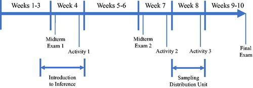
Each type of activity sequence (CSM or Hands-on) included the same time-on-task and focused on the same defined set of learning objectives. As suggested in the literature (delMas, Garfield, and Chance 1999; Chance, delMas, and Garfield 2004), both the CSM and Hands-on activities included the same preliminary questions asking students to predict the outcomes of the simulation; for example, predict the shape, center, and spread of a sampling distribution with different sample sizes. For all three activities in both treatment groups, we used the free Rossman–Chance online applets for the CSM portion of the activity1. In the CSM group, the majority of time (approximately 35 of 50 min) was spent on the applets; whereas in the Hands-on group, that same time was split between a hands-on simulation followed by the use of the applets. Students in both treatment groups received the same instruction on how to use the online applets through in-class worksheets and instructor guidance. After the activity, students in both treatment groups filled out the same set of online follow-up questions in which they reflected on the results of the simulations.

Table 1 provides a summary description of each activity in the treatment sequence. Activity 2 simulates a sampling distribution of a sample proportion from a probability model. Activities 1 and 3 perform informal randomization tests—repeatedly randomly reassigning subjects to groups under the assumption of no effect, then examining the behavior of statistics across those reassignments. Though the simulated distribution of statistics in a randomization test is not, by definition, a sampling distribution, it conveys the same principle of “sampling” variability of a statistic. For these two randomization test activities, the datasets were already built into the Rossman and Chance applets. Both sequences of discussion activity in-class worksheets (CSM and Hands-on) are available in the supplementary materials.

Table 1 Descriptions of treatment sequence discussion activities.

	Activity 1	Activity 2	Activity 3
Context	Does swimming with dolphins improve depression?	How does the proportion of orange M&M^® candies vary across samples?	Does sleep deprivation have lingering effects on visual learning?
Variables	Whether subject swam with dolphins; Whether depression symptoms improved	Whether a candy is orange	Whether subject was deprived of sleep; Improvement score on visual discrimination task
Simulated statistic	Difference in proportions	One proportion	Difference in means
Rossman and Chance applet	Randomization test for categorical response: Dolphin Study	Reeses Pieces	Randomization test for quantitative response: two means
Hands-on objects	Playing cards with red cards representing “improvers” and black cards representing “non-improvers”	M&M’s^®	Raffle tickets with observed improvement scores written on backs

2.1.2 Assignment of Treatments

Assignment of treatments to discussion sections, shown in Figure 2, was designed in such a way as to control for any instructor (TA) effect and to minimize confounding due to time of day or order of treatments. Each TA was assigned both treatments—two TAs were randomly selected to use the CSM activity in their earliest discussion (TAs 1 and 3), and the other two used the Hands-on activity in their earliest discussion (TAs 2 and 4). Though the time of day for the eight discussion sections varied, each TA taught their two discussion sections back-to-back. All TAs were given the same set of instructions for each activity and the students were blind to the study. Although the study design was not a randomized experiment since students self-selected into each discussion section, the treatments were randomly assigned to discussion sections as described above.

Fig. 2 Course schedule, treatment assignments, and sample sizes used in the analysis.

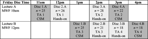
It should be noted that the assignment of treatments was performed at the section level, not at the student level. However, as with many educational studies, we use the student as our unit of analysis. This limitation should be taken into account when considering the results of this study.

2.1.3 Participation

Approximately 89% of the students participated in the first activity, 80% in the second, and 72% in the final activity. For the analysis, of the initial 436 students enrolled in the course, we removed two students from the dataset as they were simply auditing the course. We also did not include students who did not take the Final Exam (16 total), students who were taking the course for Pass/No Pass (1 total), as well as students who did not attend the same discussion section for all three activities (30 total). Finally, we removed students who did not participate in all three discussion activities, as these students did not complete the full treatment (203 total). Figure 2 includes the final sample sizes used in the analysis for each discussion section.

Table 2 summarizes the distribution of the number of discussion activities attended for those students who went to the same discussion section throughout the sequence. Unfortunately, many students did not complete the entirety of the treatment sequence. This was due to how discussion attendance grades were assigned in the course—students were only required to attend four out of five active-learning discussions for full credit (three of which were the treatment sequence). The third and final discussion in the treatment sequence was also the fifth and final active-learning discussion of the quarter. By then, many students had already fulfilled their four-discussion attendance requirement and therefore decided to skip the last activity (108 students). However, as our research question was focused on students who participated in the complete sequence of simulation activities, only those students who attended all three discussions were included in our analysis. This resulted in a substantial reduction of our sample size.

Table 2 Student participation in discussion sequence.

No. of discussions attended	0	1	2	3	Total
Student count	9	23	171	183	386

2.1.4 Assessment

Students were assessed on two in-class midterm exams and one comprehensive final exam, the activity in-class worksheets, and online written reflections after each activity. Both the in-class worksheets and online written reflections were graded based only on completion. Though each exam covered additional topics beyond sampling distributions specifically, the concept of sampling distributions underlies many of the principles in the introductory course. Thus, we viewed exam scores as an “overall” measurement of student understanding of statistical concepts. In this article, we use student exam scores, standardized such that each exam has mean zero and standard deviation one, as our primary outcome. This choice of outcome variable was partially due to the limited number of sampling distribution-specific exam questions (one multiple choice item on Midterm Exam 2, and two multiple choice and one free response item on the Final Exam). We will present a mixed-methods analysis of the activity in-class worksheets and online reflections in future work.

All students took the same set of exams. Since the treatment was not implemented until after the first exam, Midterm Exam 1 served as a baseline (see Figure 1). Thus, the statistical methods described in Section 2.2 model the difference in standardized exam score from Midterm Exam 1 to Midterm Exam 2 and to the Final Exam, respectively, rather than the standardized exam scores themselves. Prior to analysis, we hypothesized that students who participated in the hands-on activities prior to CSMs would show more improvement from Midterm Exam 1 to the Final Exam than students who participated in the CSM activities only, controlling for potential precision and confounding variables.

2.2 Statistical Methods

Since repeated measures were taken on each student, there was inherent positive correlation across each individual student’s exam scores. Therefore, we used the generalized estimating equation (GEE) framework to model the association between treatment group (Hands-on or CSM) and change in exam scores, while controlling for other covariates and accounting for correlation within individuals. GEE models are considered semiparametric in that only the mean, variance, and correlation models are specified—a complete probability distribution assumption for the response is not required. We used Wald tests with robust standard errors for inference on model coefficients.

The difference in standardized exam scores from Midterm Exam 1 to the Final Exam, and the difference from Midterm Exam 2 to the Final Exam (Final–Midterm 1, Final–Midterm 2) served as the response variable. In addition to the primary variables of interest—treatment group and a midterm exam indicator variable—we included several other covariates: TA (1, 2, 3, or 4), major (STEM or non-STEM), and sex (Male or Female). The variables major and sex were obtained through the university Registrar’s Office.

Thus, our a priori model for the mean change in standardized exam score from Midterm Exam j to the Final Exam for student i, was(1) $$\begin{array}{c}M\mathit{odel}1:\\ \mathrm{E}\left[D_{ij}\right]={\beta }_0+{\beta }_1{\text{Hands}-\text{on}}_i+{\beta }_2{\text{Mid}2}_j+{\beta }_3{\text{TA}2}_i+\\ {\beta }_4{\text{TA}3}_i+{\beta }_5{\text{TA}4}_i+{\beta }_6{\text{Male}}_i+{\beta }_7{\text{STEM}}_i+\\ {\beta }_8{\text{Hands}-\text{on}}_i\times \text{Mid}{2}_j,\end{array}$$(1)

$i=1,\dots ,183$, j = 1, 2, where model variables are defined in Table 3.

Table 3 Definitions of variables included in Model 1 for the ith student’s difference in standardized scores between the Final Exam and Midterm Exam j.

Variable	Description
Dij	Difference in standardized exam score between the Final Exam and
	Midterm Exam j (Final–Midterm j, j = 1, 2)
Hands-on i	Treatment group indicator: 1 if Hands-on; 0 if CSM
Mid2j	1 if modeling difference between Final Exam and Midterm
	Exam 2, $D_{i2}$;
	0 if difference between Final Exam and Midterm Exam 1, $D_{i1}$
TA2i	1 if attended TA 2’s discussions; 0 otherwise
TA3i	1 if attended TA 3’s discussions; 0 otherwise
TA4i	1 if attended TA 4’s discussions; 0 otherwise
Malei	1 if male; 0 otherwise
STEMi	1 if STEM field major; 0 otherwise

The primary coefficients of interest in Model 1 are those that model the difference between the two treatment groups (Hands-on–CSM) in the average difference in standardized exam score from: Midterm Exam 1 to the Final Exam (β₁), Midterm Exam 2 to the Final Exam (${\beta }_1+{\beta }_8$), and Midterm Exam 1 to Midterm Exam 2 ($-{\beta }_8$). (See Table 7 in Section 3.2 for expressions and estimates of these differences.)

Table 7 Differences between groups in the mean change in standardized exam score across exams.

Difference	Estimate	95% CI	p-value
(Final – Mid 1)${}_{\text{Hands}-\text{on}}$ – (Final – Mid 1)${}_{\text{CSM}}$	0.283	(0.052, 0.514)	0.02
(Final – Mid 2)${}_{\text{Hands}-\text{on}}$ – (Final – Mid 2)${}_{\text{CSM}}$	0.242	(0.029, 0.455)	0.03
(Mid 2 – Mid 1)${}_{\text{Hands}-\text{on}}$ – (Mid 2 – Mid 1)${}_{\text{CSM}}$	0.041	(–0.273, 0.354)	0.80

NOTE: Estimates correspond to Model 1 coefficients β₁, ${\beta }_1+{\beta }_8$, and $-{\beta }_8$, respectively.

As discussed in Section 2.1.3, poor student attendance resulted in a substantial reduction in our sample size. One approach to handling missing data of this kind is an “intent-to-treat” (ITT) analysis. The concept of ITT originated in the context of randomized controlled trials, which often suffer from noncompliance, dropout, and missing outcomes. The ITT principle assumes that, in practice, patients will behave similarly to those in the study and may not comply or continue the treatment. Thus, an analysis that excludes those patients would suffer from bias. Instead, an ITT analysis includes all participants that were originally randomized to treatments, regardless of dropout or noncompliance behavior (Gupta 2011; McCoy 2017).

In our context, we are interested in the effects of the discussion activity sequence if students were to attend all three activities, which justifies our choice to drop any students who missed an activity. However, if one were interested in the effect of the treatment on students with typical attendance behavior, then the ITT model may be more appropriate. We include the results of an ITT analysis of the complete data in Table A.1 of the Appendix.

3 Results

3.1 Descriptive Statistics

Table 4 reports exam score summary statistics, and Figure 3 displays the trajectories of the raw exam scores by treatment. It can be seen in Table 4 and Figure 3 that the average raw exam score (out of 100) for students in the CSM group steadily declined over the quarter (average decrease of 4.7 from Midterm Exam 1 to the Final Exam); however, average exam scores for students in the Hands-on group declined from the first exam to the second, but then increased after Midterm Exam 2, which resulted in only a 0.9 total decrease in average exam score from Midterm Exam 1 to the Final Exam. With this information alone, it appears that, on average, students in the CSM group had a slightly better grasp of the material in the short term, but were not able retain the information as well as students in the Hands-on group.

Fig. 3 Left: Boxplots of raw exam scores by treatment; Right: Mean raw exam score by treatment with 95% confidence intervals.

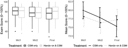
Table 4 Means and standard deviations of raw and standardized exam scores by treatment group for the 183 students included in the analysis. Raw exam scores are out of 100 points.

	CSM (n = 90)		Hands-on (n = 93)
	Mean	Std. mean	Mean	Std. mean
	(SD)	(SD)	(SD)	(SD)
Midterm Exam 1 Score	80 (11.9)	0.1 (0.9)	78.1 (14.2)	0 (1.1)
Midterm Exam 2 Score	77.9 (13.9)	0.1 (0.9)	76.4 (15.3)	0 (1.0)
Final Exam Score	75.3 (14.9)	0.0 (1)	77.2 (14.9)	0.1 (1.0)

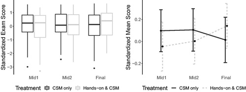
To adjust for the varying difficulty levels across exams, we modeled standardized exam scores in the analysis. For each exam, a student’s score was standardized by subtracting the overall mean for that exam, then dividing by the overall standard deviation (across both treatment groups). In Table 4, we see the same pattern in the change in standardized exam scores from Midterm Exam 2 to the Final Exam as in the raw exam scores—the mean standardized exam score of the Hands-on group increased slightly (0.1 standard deviations) from Midterm Exam 2 to the Final Exam, whereas the mean standardized exam score in the CSM group decreased by 0.1 standard deviations. The changes in these standardized exam scores over time by treatment are shown graphically in Figure 4.

Fig. 4 Left: Boxplots of standardized exam scores by treatment; Right: Mean standardized exam score by treatment with 95% confidence intervals.

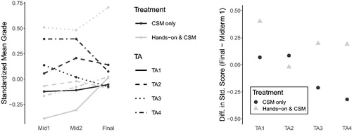
When broken down by discussion section (Figure 5), we see that there are varying patterns in average standardized exam scores over time, but for each exam these averages only varied by about one standard deviation across all sections. Figure 5 also displays the change in mean standardized exam score from Midterm Exam 1 to the Final Exam by TA and treatment, which is one of the outcomes modeled in Model 1. TAs 1, 3, and 4 exhibited a more positive change in mean standardized exam score under the Hands-on treatment, whereas TA 2 saw a slightly higher change in mean standardized exam score under the CSM treatment.

Fig. 5 Left: Mean standardized exam score by TA and treatment; Right: Difference between Midterm Exam 1 and Final Exam in mean standardized exam scores by TA and treatment.

Covariate summary statistics by treatment group are shown in Table 5. The distributions of major were similar across the treatment groups, but the CSM group had a larger percentage of females than the Hands-on group.

Table 5 Covariate summary statistics by treatment group for the 183 students included in the analysis.

	CSM (n = 90)	Hands-on (n = 93)
	n (%)	n (%)
Major
Non-STEM	60 (67%)	64 (69%)
STEM	30 (33%)	29 (31%)
Sex
Female	61 (68%)	54 (58%)
Male	29 (32%)	39 (42%)

3.2 Model Results

Results from fitting Model 1 using the differences in standardized exam scores are shown in Table 6, and Table 7 highlights the coefficients of interest. As seen in Table 7, we found discernible differences between the treatment groups in both the change from Midterm Exam 1 to the Final Exam, and the change from Midterm Exam 2 to the Final Exam, controlling for TA, sex, and major. Results suggest that, with 95% confidence, the change in mean standardized exam score from Midterm Exam 1 to the Final Exam is between 0.052 and 0.514 standard deviations higher for the Hands-on group, among students similar with respect to TA, sex, and major. Since there was only one activity between Midterm Exam 1 and Midterm Exam 2, and the sampling distribution unit was taught in lecture between Midterm Exam 2 and the Final Exam (see Figure 1), we see no statistically discernible difference between the two treatment groups in the change in mean standardized score between the two midterm exams.

Table 6 Model 1 summary.

	Estimate	Robust SE	95% CI	Robust z	p–value
Intercept	0.161	0.129	(–0.091, 0.413)	1.252	0.21
Hands-on	0.283	0.118	(0.052, 0.514)	2.403	0.02
Mid2	–0.008	0.114	(–0.231, 0.215)	–0.069	0.95
TA2	–0.252	0.112	(–0.471, –0.033)	–2.258	0.02
TA3	–0.169	0.118	(–0.399, 0.062)	–1.432	0.15
TA4	–0.306	0.118	(–0.538, –0.073)	–2.580	0.01
Male	–0.061	0.082	(–0.222, 0.101)	–0.736	0.46
STEM	–0.087	0.092	(–0.268, 0.094)	–0.945	0.35
Hands–on:Mid2	–0.041	0.160	(–0.354, 0.273)	–0.255	0.80

Holding all else constant, we found no discernible difference between males and females, or between STEM and non-STEM majors in the changes in standardized exam scores. However, there were statistically discernible differences across TAs. In fact, the interaction between TA and treatment is moderately statistically discernible (significant) (F-statistic = 0.50; p-value = 0.07) when added to Model 1, indicating that differences between treatments could depend on the TA.

As discussed in Section 2.2, we also ran an intent-to-treat (ITT) analysis, summarized in Table A.1 of the Appendix. This analysis used data from all students who attended at least one of the activities (n = 377). In the ITT model, we included the number of discussions attended (labeled “Participation” in Table A.1) as an additional quantitative variable. The primary results of interest are similar to those in Table 6. Interestingly, the effect of participation (number of discussions attended) was not statistically discernible (p-value = 0.30), suggesting that, controlling for treatment group, exam, TA, sex, and major, the number of activities attended did not have a strong association with the average change in exam score.

3.3 Sampling Distribution Assessment Items

One multiple choice item on Midterm Exam 2, and two multiple choice and one free response item on the Final Exam specifically targeted sampling distributions. On Midterm Exam 2, students were asked to identify the observational unit on a randomization distribution of binomial counts using the same context as Activity 1. The final exam included two multiple choice items from the Assessment Resource Tools for Improving Statistical Thinking (ARTIST) Sampling Variability Scale (Garfield et al. 2006), and one multi-part free response question (worth 13 points) asking students to draw, describe, and calculate probabilities from a sampling distribution of a sample mean. These four sampling distribution-specific assessment items are available in the supplementary materials. Summaries of student responses to these items are displayed in Figure 6.

Fig. 6 Results on sampling distribution-specific exam items by treatment group.

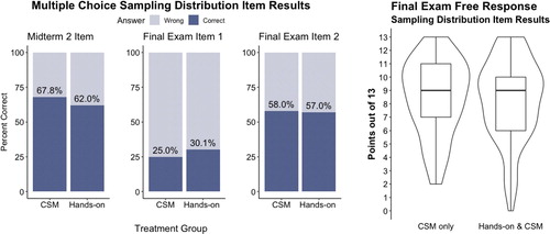
With only four items, three of which being multiple choice, it is difficult to detect any substantial differences between the treatment groups in their understanding of sampling distributions. On the multiple choice items, the CSM group performed slightly better on the Midterm Exam 2 item. However, the Hands-on group performed slightly better on the first of the final exam multiple choice items, and the two groups performed nearly the same on the second. The median score on the sampling distribution-specific free response item on the Final Exam was 9 (out of 13) for both groups, with a few particularly low scores in the Hands-on group.

4 Discussion

The goal of our analysis was to investigate if participating in hands-on simulation activities prior to performing computer simulations improves student learning of sampling distributions, as measured by exam score trajectories. We found that, while there was no statistically discernible effect of the treatment on the change in standardized exam score from Midterm Exam 1 to Midterm Exam 2 (which occurred after only one activity in the treatment sequence), there was a statistically discernible positive effect of hands-on simulations on exam score trajectories from Midterm Exam 1 and from Midterm Exam 2 to the Final Exam.

Though results were statistically discernible (significant), the effect size is equally—if not more—important. Without controlling for covariates, the average standardized exam scores decreased by about 0.1 standard deviations from Midterm Exam 1 to the Final Exam in the CSM group; whereas the average standardized exam score increased by about 0.1 standard deviations in the Hands-on group (see Table 4). This effect size of 0.2 standard deviations between the two groups is equivalent to a change of about 3% on an exam grade. Controlling for covariates, the change in average standardized exam score from Midterm Exam 1 to the Final Exam under the Hands-on treatment is between 0.05 and 0.5 standard deviations more than the CSM treatment, with 95% confidence (see Table 7), or between 0.7% and 7% in the change in exam grades. A difference of 0.7% may not matter to a student, but a difference of 7% could mean the difference between two letter grades.

This study adds empirical evidence to the recommendations for using hands-on activities prior to CSMs in the literature, though further study is needed. Exam scores measure an overall understanding of statistical concepts, but they do not specifically isolate understanding of sampling distributions. In fact, our results are somewhat surprising, as the treatment only involved three sampling distribution-focused 50-min discussion activities over an entire quarter, and exams covered a variety of topics. Moreover, on the few sampling distribution-specific exam questions, the CSM group performed slightly better on some, and the Hands-on group performed slightly better on others. Indeed, an examination of the effect of hands-on activities using an assessment instrument that directly measures understanding of sampling distributions through more than a few items is needed.

Though the study was designed to control for TA effects and other variables, the treatment is still associated with other factors. For example, during interviews with the four TAs at the end of the quarter, every TA stated that they enjoyed teaching the discussion activities that included hands-on portions more than those that only used CSMs. Additionally, all four TAs felt that the students were more engaged when the discussions included hands-on activities. Thus, whether the difference in exam trajectories between treatments was due to the hands-on activities themselves or due to increased enthusiasm from the TA and fellow students (or due to another related variable) cannot be determined. These observations, however, may serve as additional testimony in support of hands-on simulations—there are other factors besides a small increase in exam performance that might make the time used for hands-on simulations worthwhile.

In the next stage of this research, we will examine student responses to the discussion activity online reflections through a mixed-methods analysis. Reflection questions contained both multiple choice items and free response questions, some of which were motivated by items that targeted sampling distributions on the validated ARTIST Scales and Comprehensive Assessment of Outcomes in a First Statistics Course (CAOS) (Garfield et al. 2006; delMas, Garfield, and Ooms 2007). A deeper analysis of these reflections will allow us to delve into how the two treatment groups differed in their understanding of sampling distributions specifically.

In summary, the addition of hands-on activities prior to CSMs appears to have a small, positive relationship with student exam performance. Though these hands-on activities may take valuable class time, their use appears to be beneficial for the student, and can be rewarding and enjoyable for the instructor.

Supplementary Materials

The three discussion activity worksheets for each treatment group (hands-on + computer simulation; computer simulation) and the sampling distribution exam items are available in the supplementary materials.

Appendix: Additional Model Results

Table A.1 Intent-to-treat model summary.

	Estimate	Robust SE	95% CI	Robust z	p–value
Intercept	–0.153	0.155	(–0.456, 0.150)	–0.992	0.321
Participation	0.056	0.050	(–0.042, 0.153)	1.119	0.263
Hands-on	0.216	0.084	(0.051, 0.381)	2.569	0.010
Mid2	0.027	0.079	(–0.127, 0.182)	0.347	0.729
TA2	–0.052	0.086	(–0.220, 0.116)	–0.606	0.544
TA3	–0.107	0.081	(–0.267, 0.053)	–1.314	0.189
TA4	–0.037	0.087	(–0.207, 0.133)	–0.427	0.670
Male	–0.076	0.058	(–0.190, 0.039)	–1.295	0.195
STEM	–0.012	0.063	(–0.136, 0.112)	–0.192	0.848
Hands–on:Mid2	–0.040	0.115	(–0.265, 0.186)	–0.344	0.731

Acknowledgments

We would like to thank the editor and reviewers for their insightful comments and suggestions.

References

- Beckman, M. D., DelMas, R. C., and Garfield, J. (2017), “Cognitive Transfer Outcomes for a Simulation-Based Introductory Statistics Curriculum,” Statistics Education Research Journal, 16, 419–440.
- Chance, B., Ben-Zvi, D., Garfield, J., and Medina, E. (2007), “The Role of Technology in Improving Student Learning of Statistics,” Technology Innovations in Statistics Education, 1. Available at https://doi.org/https://escholarship.org/uc/item/8sd2t4rr.
- Chance, B., delMas, R. C., and Garfield, J. (2004), “Reasoning About Sampling Distributions,” in The Challenge of Developing Statistical Literacy, Reasoning and Thinking, eds. D. Ben-Zvi and J. Garfield, Dordrecht: Springer, pp. 295–323.
- Chance, B., Garfield, J., and delMas, R. (2000), Developing Simulation Activities to Improve Students’ Statistical Reasoning, Auckland, New Zealand: Aukland University of Technology.
- delMas, R., Garfield, J., and Chance, B. L. (1999), “A Model of Classroom Research in Action: Developing Simulation Activities to Improve Students’ Statistical Reasoning,” Journal of Statistics Education, 7.
- delMas, R., Garfield, J., and Ooms, A. (2007), “Assessing Students’ Conceptual Understanding After a First Course in Statistics,” Statistics Education Research Journal, 6, 28–58. Available at https://doi.org/http://jse.amstat.org/secure/v7n3/delmas.cfm.
- Dyck, J. L., and Gee, N. R. (1998), “A Sweet Way to Teach Students About the Sampling Distribution of the Mean,” Teaching of Psychology, 25, 192–195.
- GAISE College Report ASA Revision Committee (2016), “Guidelines for Assessment and Instruction in Statistics Education College Report 2016,” Technical Report.
- Garfield, J., and Ben-Zvi, D. (2007), “How Students Learn Statistics Revisited: A Current Review of Research on Teaching and Learning Statistics,” International Statistical Review/Revue Internationale de Statistique, 75, 372–396.
- Garfield, J., delMas, R., Chance, B., and Ooms, A. (2006), “Assessment Resource Tools for Improving Statistical Thinking (ARTIST) Scales and Comprehensive Assessment of Outcomes in a First Statistics Course (CAOS) Test,” available at https://doi.org/https://apps3.cehd.umn.edu/artist/caos.html.
- Gourgey, A. F. (2000), “A Classroom Simulation Based on Political Polling to Help Students Understand Sampling Distributions,” Journal of Statistics Education, 8. Available at https://doi.org/http://jse.amstat.org/secure/v8n3/gourgey.cfm.
- Gupta, S. K. (2011), “Intention-to-Treat Concept: A Review,” Biostatistics, 2, 109–112.
- Hodgson, T. (1996), “The Effects of Hands-on Activities on Students’ Understanding of Selected Statistical Concepts,” in Proceedings of the Eighteenth Annual Meeting of the North American Chapter of the International Group for the Psychology of Mathematics Education, Columbus, OH, pp. 241–246. ERIC Clearinghouse for Science, Mathematics, and Environmental Education.
- Lane, D. M. (2015), “Simulations of the Sampling Distribution of the Mean Do Not Necessarily Mislead and Can Facilitate Learning,” Journal of Statistics Education, 23. Available at https://doi.org/10.1080/10691898.2015.11889738.
- McCoy, E. C. (2017), “Understanding the Intention-to-Treat Principle in Randomized Controlled Trials,” Western Journal of Emergency Medicine, 18, 1075–1078.
- Meletiou-Mavrotheris, M. (2003), “Technological Tools in the Introductory Statistics Classroom: Effects on Student Understanding of Inferential Statistics,” International Journal of Computers for Mathematical Learning, 8, 265–297.
- Mills, J. D. (2002), “Using Computer Simulation Methods to Teach Statistics: A Review of the Literature,” Journal of Statistics Education, 10. Available at https://doi.org/10.1080/10691898.2002.11910548.
- Pfaff, T. J., and Weinberg, A. (2009), “Do Hands-on Activities Increase Student Understanding?: A Case Study,” Journal of Statistics Education, 17. Available at https://doi.org/10.1080/10691898.2009.11889536.
- Saldanha, L., and Thompson, P. (2007), “Exploring Connections Between Sampling Distributions and Statistical Inference: An Analysis of Students’ Engagement and Thinking in the Context of Instruction Involving Repeated Sampling,” International Electronic Journal of Mathematics Education, 2, 270–297.
- Schwarz, C. J., and Sutherland, J. (1997), “An On-Line Workshop Using a Simple Capture-Recapture Experiment to Illustrate the Concepts of a Sampling Distribution,” Journal of Statistics Education, 5. Available at https://doi.org/10.1080/10691898.1997.11910523.
- Sotos, A. E. C., Vanhoof, S., Van den Noortgate, W., and Onghena, P. (2007), “Students’ Misconceptions of Statistical Inference: A Review of the Empirical Evidence From Research on Statistics Education,” Educational Research Review, 2, 98–113.
- Utts, J. M., and Heckard, R. F. (2015), Mind on Statistics (5th ed.), Boston, MA: Cengage.
- Watkins, A. E., Bargagliotti, A., and Franklin, C. (2014), “Simulation of the Sampling Distribution of the Mean Can Mislead,” Journal of Statistics Education, 22. Available at https://doi.org/10.1080/10691898.2014.11889716.
- Watson, J., and Chance, B. (2012), “Building Intuitions About Statistical Inference Based on Resampling,” Australian Senior Mathematics Journal, 26, 6–18.
- Weir, C. G., McManus, I. C., and Kiely, B. (1991), “Evaluation of the Teaching of Statistical Concepts by Interactive Experience With Monte Carlo Simulations,” British Journal of Educational Psychology, 61, 240–247.
- Wood, M. (2005), “The Role of Simulation Approaches in Statistics,” Journal of Statistics Education, 13. Available at https://doi.org/10.1080/10691898.2005.11910562.
- Zerbolio Jr., D. J. (1989), “A ‘Bag of Tricks’ for Teaching About Sampling Distributions,” Teaching of Psychology, 16, 207.