Introducing Undergraduates to Concepts of Survey Data Analysis

Abstract

Increasingly students, particularly those in the social sciences, work with survey data collected through a more complex sampling method than a simple random sample. Failing to understand how to properly approach survey data can lead to inaccurate results. In this article, we describe a series of online data visualization applications and corresponding student lab activities designed to help students and teachers of statistics better understand survey design and analysis. The introductory and advanced materials presented are designed to focus on a conceptual understanding of survey data and provide an awareness of the challenges and potential misuse of survey data. Suggestions and examples of how to incorporate these materials are also included. Supplementary materials for this article are available online.

KEYWORDS:

• Political poll
• Shiny app
• Survey weights
• Statistics education

1 Introduction

Introductory statistics courses and popular introductory textbooks (Gould and Ryan 2015; Tintle et al. 2016; Lock et al. 2017) primarily focus on the analysis of data obtained from a simple random sample (SRS) or a randomized experiment. Typically there is no more than one section about data collection focused on defining and discussing differences between an SRS and the use of stratification, clustering, or probabilistic methods. Actual analysis of data from a design other than an SRS typically only appears in upper level courses or at the graduate level. However, with the abundance and availability of data and the growing use of data to support learning and decision-making across disciplines, it is becoming increasingly important that all statistics students recognize common challenges that occur with complex data. In particular, in the social sciences, it is very common for market researchers, government organizations, and political pollsters to over-sample some subgroups of the population. Students in these fields typically only take one statistics course and fail to understand how to properly treat survey data that were collected through stratified random samples. This can lead to inaccurate results in their future work (Gelman 2007).

While introductory statistics courses are often students’ last exposures to a formal statistics course, it is not the last time they are presented with data and statistics. Switzer and Horton highlight the growing disparity in the medical field between the content of introductory courses and the statistical methods used in original articles in the New England Journal of Medicine (NEJM). “Readers with knowledge of only the topics typically included in introductory statistics courses may not fully comprehend a large fraction of the statistical content of original articles in the NEJM” (Switzer and Horton 2007, p. 17). Similar disparities are likely to be present in many other fields, including areas that primarily utilize survey data. Furthermore, there is a growing availability of survey data involving politics, the economy, health, education, demography, social behaviors, and a myriad of other government data. However, the Pew Research Center for the People and Press states “Political and media surveys are facing significant challenges as a consequence of societal and technological changes… The general decline in response rates is evident across nearly all types of surveys, in the United States and abroad…. Despite declining response rates, telephone surveys that include landlines and cell phones and are weighted to match the demographic composition of the population continue to provide accurate data on most political, social, and economic measures” (Kohut et al. 2012, p. 1). Students today are facing an increased exposure to and use of survey data. Survey data are also more complex in design and analysis (including proper use of survey weights). Thus, there is a clear need to provide an awareness of the challenges in interpreting and properly working with survey data to undergraduate students.

In this article, we describe a series of online data visualization applications and corresponding student lab activities designed to describe survey design concepts and highlight the importance of the entire process, including design, data collection, analysis, and communication of the results. These activities are designed to gradually introduce students to the analysis of data that do not come from an SRS. The materials do not provide a cookbook guide to analyzing survey data, but instead lead students through conceptual understanding of survey data and the importance of incorporating sample selection into the analysis.

The first activity described below is appropriate for any first course in statistics and uses visualizations to emphasize the potential errors that can occur when we treat survey data as if it came from an SRS. Our second activity uses actual survey data on political preferences and can be used to demonstrate how easily political surveys can be misunderstood. This activity would be appropriate for a first or second course in statistics as well as for courses in subject-matter disciplines that utilize survey data (e.g., political science). Three additional activities are more appropriate for more advanced statistics or social science courses. They involve additional survey data from politics, alternative medicine, and the National Health and Nutrition Examination Survey (NHANES).

2 Should It Pass? An Introduction to the Challenges of Weighted Data

To introduce students to the idea of weighted data, we created freely available interactive data visualizations to demonstrate how population estimates can be influenced by the sample selection. By the end of this activity, we expect students to be able to understand the following core concepts:

• A stratified random sample involves dividing the population of interest into several smaller groups, called “strata,” and then taking an SRS from each of these smaller groups.

• This method is commonly used when we want to guarantee a large enough sample from each subgroup.

• When this type of sampling method is used, it is important to use weights to account for the relative size of each subgroup. Weights are values assigned to individuals in a sample based upon how representative the individual is of the total population.

• When used appropriately, weighted data can provide more accurate population estimates than unweighted data.

The activity begins by introducing a hypothetical situation where students at a local university would like to pass a resolution to increase tuition costs to hire two statistical consultants to help with graduate research. The graduate program has a total of 1000 students and the undergraduate program has a total of 20,000 students. For this resolution to pass, at least 50% of the entire student body must support it.

A survey was conducted of 200 students asking them to indicate whether or not they would support this resolution. If the sample was from an SRS, we would expect only 4.8% = 1000/21,000 (i.e., 9 or 10 students) out of the sample of 200 to be graduate students. To ensure that both student groups were well represented in the survey, a stratified random sample was used; 100 graduate students and 100 undergraduates were randomly selected to complete the survey. This survey resulted with 110 responding “yes” and 90 responding “no,” results summarized in Table 1.

Table 1 Summary table showing the results from the hypothetical university survey.

	Yes	No	Total
Undergraduate	30	70	100
Graduate	80	20	100
Total	110	90	200

If the data were evaluated assuming they came from an SRS, the estimated proportion in support of the resolution would be 55% (110/200). Based on this information, one would most likely conclude that this resolution does appear to have enough support to pass. However, this conclusion is only appropriate if the students sampled were an accurate representation of the total student body. By including 100 graduate students in the sample, we can better understand the graduate student view of the resolution compared to the information provided by only 9 or 10 students. However, the graduate students are overrepresented in the sample compared to the population.

While the sample sizes ensure that each subgroup (undergraduate and graduate) provide fairly reliable estimates, students quickly see that 55% is not a reliable point estimate of the overall percentage who would agree with this resolution. We then demonstrate to students how to use the population sizes as weights to obtain a better estimate of the percentage of students who support the resolution. In the sample, 30% of the undergraduate students and 80% of graduate students responded with a “yes” to the survey. An estimated 6000 (20,000 × 0.30) undergraduate students and an estimated 800 (1000 × 0.80) graduate students would support the resolution. Thus, when we account for the sample selection by adjusting or weighting each response, we estimate that approximately 32% (6800/21,000) of the entire student body supports the resolution. Students are then asked to discuss how failing to account for the sample selection and weighting can lead to results that are not truly representative of the entire population. This example demonstrates the importance of accounting for weights in survey data. When using a stratified sample, population estimates can be dramatically biased if weights are ignored, particularly when the responses vary between strata.

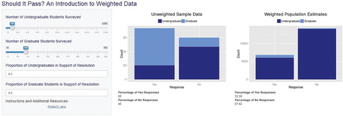
After working through the above example, students are then directed to the Should It Pass? ShinyApp, shown in Figure 1, which allows them to interactively modify the sample selection of each subgroup and view the unweighted and weighted results. Exploring the app helps students further grasp the role of subgroups and weights on estimates. They are encouraged to explore the app to discover under what conditions the unweighted and weighted estimates are very similar or when they provide very different results.

Fig. 1 Screenshot from the Should It Pass? ShinyApp that allows students to modify the hypothetical survey design by adjusting the sample sizes of each strata. Students can also modify the proportion in each group that support the resolution. Graphs display the unweighted sample data and the weighted population estimates allowing students to compare the unweighted results and weighted estimates for the specified situation. This app as well as corresponding datasets and student lab handout are freely available at https://stat2labs.sites.grinnell.edu/weights.html.

In this activity, we also demonstrate that survey data are generally available with individual entries as opposed to the summary table of counts as given above in Table 1. The first 6 rows of the full dataset are given in Table 2.

Table 2 First six rows of the university survey data demonstrating the use of weights.

ID	Status	Vote	Weight	Weighted vote
1	Undergraduate	0	200	0
2	Graduate	1	10	10
3	Undergraduate	1	200	200
4	Undergraduate	1	200	200
5	Graduate	0	10	0
6	Graduate	1	10	10
$\dots$	$\dots$	$\dots$	$\dots$	$\dots$
Sum		110	21,000	6800

NOTE: The sum of each column based upon all 200 cases in the sample is also shown.

Table 2 includes a weight variable that can be used to scale the sample up to the population size. A sample of 100 graduate students was obtained from the total 1000 graduate student body so each graduate student in the sample would represent 10 (1000/100) graduate students in the population. Thus, we can assign a value of 10 as the weight of each graduate student. Similarly the weight of each undergraduate response would be given a weight of 200 (20,000/100). Summing this weight column would give the population size. Multiplying each student’s vote (1 represents a “yes” vote, 0 represents a “no” vote) by the weight assigned to that student gives a weighted vote. Summing the weighted votes gives us a value of 6800 for the estimated weighted total number of “yes” votes. This results in the weighted estimate 32% = 6800/21,000 of the entire student body in support of the resolution. While this example is oversimplified, it has been extremely useful in helping students at all levels recognize the consequences of ignoring weights on point estimation. While we do not expect most students in our introductory classes to work intensely with weighted data, we should expect them to be able to question any results based on survey data that did not incorporate weights into the analysis.

3 Political Preferences 1: Using Weights to Evaluate Political Preferences

Political polls are of interest to many students and there are few activities that demonstrate how to properly understand this data. Gourgey (2000) shared a nice example of understanding standard errors in political polls. However, that activity assumes that an SRS is used. To further the discussion of weighted survey data, we have created a second lab activity that examines data from a national phone survey conducted in 2010 by CBS News and the New York Times (2012). This political preference dataset reflects the type of data many students see outside of a statistics class. It offers a variety of variables to examine such as race, sex, age, religion, and political preference. It also includes a weight variable and a brief description of the survey.

Similar to the first activity, students analyze the data with and without including the weighted variable and then compare the results. Specifically, students are asked to explore differences in political preference by race. By constructing a two-way table and a visualization, students quickly see that race subgroups have strong differences in political preferences and the unweighted and weighted results give different estimated proportions.

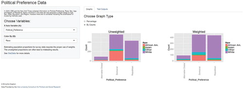
The poll specifically states there was an oversample of African Americans: the sampled proportion of African Americans was 23% compared to a US population proportion of about 14%. Students are then directed to the Political Preferences 1 ShinyApp, shown in Figure 2, to visualize and verify their work using this simple, interactive platform. There are additional opportunities to further investigate the data. For example, students can compare the unweighted and weighted results for several other subgroups provided in the dataset, including sex, income, and region.

Fig. 2 Screenshot from the interactive Political Preferences 1 ShinyApp which demonstrates that results weighted by race have much higher estimated Republican responses than the unweighted sample data. The variable displayed on the x-axis and the subgrouping variable can be changed to explore the dataset. The results can be shown in counts, as selected in the screenshot, or in percentages. This app as well as corresponding datasets and student lab handout are freely available at https://stat2labs.sites.grinnell.edu/weights.html.

Highlighting the complexities of survey data, particularly that from a political poll as in this example, is timely and relevant considering the attention on polls from recent elections across the globe. Below we list several recent articles that can be incorporated as reading and discussion assignments in an introductory course.

• After the 2016 presidential election, a New York Times article explained that many pollsters did not weight their state surveys by level of education (Cohn 2017). The article stated, “It’s no small matter, since well-educated voters are much likelier to take surveys than less educated ones. About 45% of respondents in a typical national poll of adults will have a bachelor’s degree or higher, even though the census says that only 28% of adults (those 18 and over) have a degree. Similarly, a bit more than 50% of respondents who say they’re likely to vote have a degree, compared with 40% of voters in newly released 2016 census voting data.”

• Just before the 2016 election, two articles by Cohn (2016a, 2016b) discussed the difficulty of properly weighting data. The second article described how five distinct organizations calculated different election predictions using exactly the same polling data. He explained that weighting can cause very different results, even when all groups were using exactly the same data. “The pollsters made different decisions in adjusting the sample and identifying likely voters. The result was four different electorates, and four different results” (Cohn 2016a). Andrew Gelman was part of one of the groups mentioned by Cohn (2016a) and he also discussed the differences in the predictions (Gelman 2016).

• Two articles from fivethirtyeight.com discuss the polls leading up to the 2016 U.S. Presidential election and the 2017 U.K. election and the importance of considering the variability associated within a poll (i.e., sampling variability of estimates) as well as the variability between polls (i.e., differences in sampling methods) (Silver 2016; Enten and Silver 2017). In particular, the article on the U.K. election states the following about a conservative underestimation in 2015: “…the error had more to do with the fact that the initial samples were unrepresentative of the overall population” (Enten and Silver 2017).

None of the examples in these articles discuss how to create weights for survey data. Instead, they emphasize the importance of properly considering weights when working with survey data. By incorporating these activities into a first or second statistics course (or even a political science course), students are exposed to meaningful examples of stratified random samples.

4 Assessment

The Should it Pass? and the Political Preferences 1 activities were formally class tested during the fall 2015 semester at Grinnell College. Both activities were incorporated into two sections of an introductory statistics course and two sections of a second-semester upper level statistics course. Confidential student feedback was collected through a pre- and post-quiz in all four sections. Following our IRB process, students were aware these quizzes were confidential and not graded, so the response rates were fairly low. The introductory applied statistics course had three 80-min class sessions weekly for 14 weeks. Each section had 26 students. While no calculus is used in the course, most students have taken calculus I. This course contained roughly equal amounts of lecture and lab activities. The textbook for this course was Introduction to the Practice of Statistics (Moore, McCabe, and Craig 2009).

Statistical modeling is an applied course with one introductory statistics course as a prerequisite. This course is capped at 20 students and focuses on proper data analysis for research in multiple disciplines. Historically, 75% of the students enrolled in this course have majors outside the mathematics and statistics department. Using the text, Practicing Statistics (Kuiper and Sklar 2012), the course had three 50-min class sessions weekly for 14 weeks.

In all four sections, a pre-quiz was completed as an online, out-of-class assignment prior to the activity. The class began with a short discussion and quick work through of the Should It Pass? activity including some time spent using the accompanying ShinyApp. In small groups, students then worked on their own through the Political Preferences 1 activity. Students who did not complete the activity during class were allowed to complete the work outside of class and submit it the following class period. Students were then asked to complete the online post-quiz after the second class session. Table 3 displays the results from a subset of the survey questions.

Table 3 The percentage of students who were able to properly complete the activities in the pre- and post-quiz related to weighted data.

Questions	Introductory statistics		Statistical modeling
	Pre ($n = 42$ )	Post ($n = 17$ )	Pre ($n = 32$ )	Post ($n = 22$ )
(1) Calculate unweighted estimates.	93	88	97	100
(2) Calculate weighted estimates.	24	50	62	84
(3a) Identified that unweighted estimates would lead to incorrect results.	61	75	91	95
(3b) Identified that the sample did not properly represent the population.	43	59	73	93

The number of students who correctly calculated weighted estimates was rather high for an introductory pretest (24%). However, both sections of this introductory course consist of fairly strong students who have selected to take a fast-paced course (designed for students who have already completed calculus I). Even if students did not know how to calculate weighted estimates, many were able to identify that basic unweighted data would lead to misleading results. Several additional survey questions were asked about what students liked from this activity. All 39 students who completed the post-quiz survey stated that they believed we should use these materials the next time we teach these courses.

5 Advanced Exercises

In addition to the two examples shown above, we have created three activities appropriate for an intermediate or advanced undergraduate course. The previous introductory examples focused only on point estimation, while the advanced examples also include the use of hypothesis testing with categorical weighted data. Each activity has an accompanying ShinyApp for the visualizations and chi-square test results.

1. Political Preferences 2: Weighted hypothesis tests with R instructions. This activity uses the same data as the Political Preferences 1 activity discussed above. Three different methods for analyzing the data with a chi-square test are explored: SRS method, raw weight method, and Rao–Scott method. The SRS method assumes the sample is representative of the population and uses the data unadjusted, the raw weight method creates a weighted response for each entry and then analyzes the weighted variable, and the Rao–Scott method (Rao and Scott 1981, 1984) uses the weighted variable but also takes into account how the survey design and weights will affect the variability by incorporating a design effect.

2. Complementary and Alternative Medicine (CAM): Weighted estimates and hypothesis tests with R instructions. This activity focuses on data from the 2012 Complementary and Alternative Medicine (CAM) Survey conducted by the National Center for Health Statistics. This single activity covers both the estimation and hypothesis testing concepts mentioned in the Political Preferences 1 and 2 activities. This activity would work well as a one day quick introduction to weighted data analysis.

3. NHANES (Health): Weighted estimates and hypothesis tests with R instructions. This activity uses data from a health and nutrition survey conducted by the National Center for Health Statistics which is available within the MOSAIC Package in R. This activity is very similar to the CAM activity but utilizes a much larger dataset.

We also provide advanced supplements that describe the (1) mathematical details of the Rao–Scott method and (2) types of weights, subsetting, strata, and clustering. All of these materials are freely available on our weighted data site, https://stat2labs.sites.grinnell.edu/weights.html.

6 Additional Topics

6.1 Variance Estimation

The examples presented in this article discuss how the use of weights can improve our point estimates by taking into account how the data were collected and appropriately using the weight variable. However, it is important to recognize that sampling schemes other than an SRS will also impact the variability of the estimates.

6.1.1 Unweighted Variance

After working through the proper calculation of the estimated proportion in support $(\widehat{p}=0.324)$

in the Should It Pass? activity, a naïve way to calculate the variance is to use the typical variance of a proportion equation on the weighted estimate. The following equations calculate the estimated variance and standard error of this proportion ignoring the stratified sampling design:$$\begin{array}{c}{\widehat{\sigma }}^2=\frac{\widehat{p}(1-\widehat{p})}{n}=\frac{0.324(1-0.324)}{200}\cong 0.0011,\\ {\text{SE}}_{\widehat{p}}=\sqrt{{\widehat{\sigma }}^2}=\sqrt{0.0011}\cong 0.0331.\end{array}$$

A 95% confidence interval about the point estimate could also be constructed: $$\begin{array}{c}\widehat{p}\pm 1.96\times {\text{SE}}_{\widehat{p}},\\ (0.259,0.389).\end{array}$$

6.1.2 Stratified Design Variance

To properly estimate the variance under the stratified sampling design used in the Should It Pass? activity, within-strata variances are calculated, weighted, and then summed. The weight assigned to each stratum variance is the squared proportion of the entire population in the stratum. The following equations calculate the estimated variance and standard error for this example:$$\begin{array}{c}{\widehat{\sigma }}^2\left(\widehat{p}\right)=\sum _{i=1}^s{\left(\frac{N_i}{N}\right)}^2{\widehat{\sigma }}^2\left({\widehat{p}}_i\right),i=\text{strata}1,2,\dots ,s,\\ {\widehat{\sigma }}^2\left(\widehat{p}\right)={\left(\frac{20,000}{21,000}\right)}^2\times \frac{0.30\times 0.70}{100}\\ \mathrm{\hspace{1em}}\mathrm{\hspace{1em}}+{\left(\frac{1000}{21,000}\right)}^2\times \frac{0.80\times 0.20}{100},\\ {\widehat{\sigma }}^2\left(\widehat{p}\right)={\left(0.953\right)}^2\times 0.0021+{\left(0.047\right)}^2\times 0.0016\cong 0.0019,\\ {\text{SE}}_{\widehat{p}}=\sqrt{{\widehat{\sigma }}^2}=\sqrt{0.0019}\cong 0.0437.\end{array}$$

A 95% confidence interval could also be constructed$$\begin{array}{c}\widehat{p}\pm 1.96\times {\text{SE}}_{\widehat{p}},\\ (0.238,0.410)\end{array}$$

This example highlights the importance of considering the sampling design in all calculations. There is more variability associated with the undergraduate estimate and their stratum makes up a larger portion of the entire population. The variability is underestimated when the stratified design is not incorporated into the variance calculation.

Estimation of variance is more intricate than estimation of means or totals, particularly for more complex sampling designs or other types of parameters. Gelman (2007) and Kott (2007) articulate the challenges of variance estimation in more advanced survey data techniques, such as when estimating regression coefficients. Lohr (2010) discusses several methods for estimating variances of estimated statistics from complex surveys.

6.2 Sample Allocation

The Should It Pass? activity used equal allocation where sample sizes are the same for every stratum. Another allocation method used by surveys is proportional allocation, where the sample sizes are proportional to the size of the stratum. There are additional allocation methods that take into consideration additional characteristics such as the variability within strata, model or parameter precision, and cost. The Should It Pass? ShinyApp could be used to explore different allocation methods at a basic level, as the ShinyApp does allow for users to specify individual stratum sample sizes.

6.3 Assigning Survey Weights

Weights allow sample statistics to better represent the population on a select set of demographic characteristics. However, improperly chosen weights can also lead to incorrect estimates. This topic can be discussed within the Political Preferences 1 activity. The Cohn (2017) article provided to accompany the Political Preferences 1 activity emphasized that failing to use education level within the analysis led many political pollsters to inaccurately predict the 2016 presidential election. The choice of variables included in the weighting are typically more significant than the choice of method (Kalton and Flores-Cervantes 2003).

Assigning weights are straightforward when there is only one demographic characteristic of interest such as in the Should It Pass? activity. When multiple demographic characteristics exist, such as in the Political Preferences 1 activity, proper assignment of weights generally requires iterative computational techniques to ensure that each variable of interest has the proper weight. With an increased availability of auxiliary information, more complex weighting adjustments are being developed and applied. As with any statistical technique, weight assignment methods have limitations (e.g., adjusting for noncoverage or correcting on factors with unknown population benchmarks) and assumptions (e.g., no interaction within the incorporated demographic characteristics) which need to be carefully considered and evaluated (DeBell 2018, Kalton and Flores-Cervantes 2003). With the growing complexity of survey data and the numerous weighting methods which also vary in complexity, there are clear challenges and no consensus on how to properly assign weights (Kalton and Flores-Cervantes 2003; Gelman 2007). Thus, our activities focus on the process of analyzing data where weights are already supplied, instead of addressing the weight assignment process.

7 Discussion

The goal of this article is to bring awareness of the challenges of analyzing survey data and provide examples and materials that can be easily used in the classroom. The first two examples discussed above include student handouts, interactive ShinyApps, and datasets that are appropriate for most first or second statistics courses. These two labs certainly do not provide a comprehensive explanation of analysis of survey data, but do provide an awareness of the challenges and potential misuse of weighted data. The introductory activities focus on point estimation and do not require previous inference knowledge. Alternatively, if inference methods have already been covered, the activity could be followed by discussions about how the challenges of working with survey data for point estimation would also impact inference methods. The data in the more advanced labs have multiple variables, allowing students the ability to conduct their own unique research project with the data after completing the student handout. When we tested these materials in both a first and second statistics course, students responded favorably to the materials during class testing and unanimously agreed the materials should continue to be used in future semesters of the courses. Future research could more rigorously evaluate specific learning outcomes related to the materials.

It is important to recognize that there are a wide variety of types of analysis of weighted data, and the analysis is heavily dependent upon how the data were collected. It is crucial for one to be able to recognize when the data came from a complex survey design and the implications of the design on the analysis. This is important for both individuals working with and analyzing the data as well as the general consumer reading and interpreting for themselves the results from an analysis. As Gelman states, “Survey weighting is a mess” (Gelman 2007, p. 153). The misuse of weighted data is very prevalent in many fields, and to completely ignore the consequences of this misuse is a disservice to our students. Exposing students to a dataset from a stratified random sample at a basic level deepens their understanding of working with complex data and their statistical literacy.

Supplementary Materials

List of available activities and corresponding resources.

Acknowledgments

The authors gratefully acknowledge Ruby Barnard-Mayers and Karin Yndestad for their contributions to the project as well as the anonymous reviewers and associate editor for their helpful comments and suggestions.

References

- CBS News and The New York Times (2012), CBS News/New York Times Monthly Poll #4, October 2010, Ann Arbor, MI: Inter-University Consortium for Political and Social Research [distributor], DOI: 10.3886/ICPSR33183.v1.
- Cohn, N. (2016a), “We Gave Four Good Pollsters the Same Raw Data. They Had Four Different Results,” The New York Times, September 20.
- ——— (2016b), “How One 19-Year-Old Illinois Man Is Distorting National Polling Averages,” The New York Times, October 12.
- ——— (2017) “A 2016 Review: Why Key State Polls Were Wrong About Trump,” The New York Times, May 31.
- DeBell, M. (2018), “Computation of Survey Weights,” in The Palgrave Handbook of Survey Research, eds. D. L. Vannette and J. A. Krosnick, Cham: Palgrave Macmillan, pp. 519–527.
- Enten, H., and Silver, N. (2017), “The U.K. Election Wasn’t That Much of a Shock,” FiveThirtyEight [blog], June 9, available at https://fivethirtyeight.com/features/uk-election-hung-parliament/.
- Gelman, A. (2007), “Struggles With Survey Weighting and Regression Modeling,” Statistical Science, 22, 153–164. DOI: 10.1214/088342306000000691.
- ——— (2016), “Trump +1 in Florida; or, a Quick Comment on that ‘5 Groups Analyze the Same Poll’ Exercise,” Statistical Modeling, Causal Inference, and Social Science [blog], September 23, available at https://statmodeling.stat.columbia.edu/2016/09/23/trump-1-in-florida-or-a-quick-comment-on-that-5-groups-analyze-the-same-poll-exercise/.
- Gould, R., and Ryan, C. N. (2015), Introductory Statistics: Exploring the World through Data (2nd ed.), Boston, MA: Pearson.
- Gourgey, A. F. (2000), “A Classroom Simulation Based on Political Polling to Help Students Understand Sampling Distributions,” Journal of Statistics Education, 8, 1–10.
- Kalton, G., and Flores-Cervantes, I. (2003), “Weighting Methods,” Journal of Official Statistics, 19, 81.
- Kohut, A., Keeter, S., Doherty, C., Dimock, M., and Christian, L. (2012), Assessing the Representativeness of Public Opinion Surveys, Washington, DC: Pew Research Center.
- Kott, P. S. (2007), “Clarifying Some Issues in the Regression Analysis of Survey Data,” Survey Research Methods, 1, 11–18.
- Kuiper, S., and Sklar, J. (2012), Practicing Statistics: Guided Investigations for the Second Course, Boston, MA: Pearson Addison-Wesley.
- Lock, R. H., Lock, P. F., Morgan, K. L., Lock, E. F., and Lock, D. F. (2017), Statistics: Unlocking the Power of Data (2nd ed.), Hoboken, NJ: Wiley.
- Lohr, S. L. (2010), Sampling: Design and Analysis (2nd ed.), Boston, MA: Cengage Learning.
- Moore, D. S., McCabe, G. P., and Craig, B. A. (2009), Introduction to the Practice of Statistics (6th ed.), New York: Freeman.
- Rao, J. N., and Scott, A. J. (1981), “The Analysis of Categorical Data From Complex Sample Surveys: Chi-Squared Tests for Goodness of Fit and Independence in Two-Way Tables,” Journal of the American Statistical Association, 76, 221–230. DOI: 10.1080/01621459.1981.10477633.
- ——— (1984), “On Chi-Squared Tests for Multiway Contingency Tables With Cell Proportions Estimated From Survey Data,” The Annals of Statistics, 12, 46–60.
- Silver, N. (2016) “Election Update: The Polls Disagree, and That’s OK,” FiveThirtyEight [blog], October 27, available at https://fivethirtyeight.com/features/election-update-the-polls-disagree-and-thats-ok/.
- Switzer, S. S., and Horton, N. J. (2007), “What Your Doctor Should Know About Statistics (but Perhaps Doesn’t…),” Chance, 20, 17–21. DOI: 10.1080/09332480.2007.10722826.
- Tintle, N., Chance, B. L., Cobb, G. W., Rossman, A. J., Roy, S., Swanson, T., and VanderStoep, J. (2016), Introduction to Statistical Investigations, Hoboken, NJ: Wiley.