Helping Introductory Statistics Students Find Their Way Using Maps

ABSTRACT

Maps are a primary method of displaying statistical data that comes from a geographical frame. Maps are esthetically appealing and make it easier to identify geographic patterns in a dataset. However, few introductory statistical texts and courses explicitly present maps as a way to display data. In this article, we will present examples of different types of statistical maps and illustrate how these maps can be used in the instruction of an introductory statistics course.

KEYWORDS:

• Correlation
• Descriptive statistics
• Map
• plotly
• Simple linear regression

1 Introduction

Maps are not only navigational tools; they are also important visualizations of data. Maps present all types of information: political, historical, topographic, ethnic, religious, economic, and military information, to name but a few. Every day we are bombarded with maps used by advertisers, governments, journalists, academics, and everyday people for a myriad of reasons. Like all well-done statistical visualizations, maps are “worth a thousand words” in that they can convey a dataset’s primary message much more easily than tabulations or verbal descriptions of the same data. Maps have great visual power and are capable of conveying information with incredible authority, whether real or illusory.

In this article, we argue that maps must be part of the introductory statistics curriculum. Few statistical texts explicitly present maps, so we offer examples, definitions, and an activity related to them. In Section 1.1, we argue that the ability to read maps is an essential quantitative literacy (QL) skill. Section 1.2 describes how teaching maps aligns with the Guidelines for Assessment and Instruction in Statistics Education (GAISE) College Report, which contains widely cited recommendations on what should be taught in undergraduate introductory statistics courses and how these courses should be taught. In Section 1.3, we introduce the compelling historical example of Dr. John Snow making his case for cholera as a water-borne disease through his cholera map of London, which revolutionized the field of epidemiology. Section 2 provides definitions and examples of different types of thematic maps (including the commonly used choropleth map), as well as how to interpret these maps. Section 3 describes how the topic and maps might fit into the introductory statistics curriculum and provides an example activity that examines the obesity and poverty rate by U.S. state. We provide concluding remarks in Section 4.

1.1 Maps and Quantitative Literacy

Introductory statistics courses serve as General Education requirements for many students, in which the emphasis is QL. Steen (2001) presented a characterization of QL as an “aggregate of skills, knowledge, beliefs, dispositions, habits of mind, communication capabilities, and problem-solving skills that people need to engage effectively in quantitative situations arising in life and work.” Universities place a high priority on improving the QL of all of their baccalaureate students, as there is a consensus that QL skills are invaluable to an individual’s academic career and professional life.

Statistics can be described as the science of collecting, organizing, and interpreting data. As such, the practice of statistics is an application of QL. Statistics educators should cultivate in our students the skills of inquiry and reflection, encouraging our students to employ statistical science to be creative and productive citizens.

As we demonstrate in this article, maps are extensively used to articulate arguments related to geographic data. Given their frequency of use, the authors of this article believe that maps should be discussed in introductory statistics courses. Further, we would encourage authors of introductory statistics texts to infuse examples of the use of maps in their text. This will encourage statistics faculty to discuss maps in their courses. As statistics educators, we should be preparing our students to interpret maps and identify their associated strengths, weaknesses, and potential biases.

1.2 Maps and the GAISE Report

The GAISE College Report (GAISE College Report ASA Revision Committee 2016) discusses mapping under the fifth of its overarching recommendations, to “use technology to explore concepts and analyze data” (p. 3). The report says that mapping is an “increasingly common visualization that is intuitive and insight-provoking, though statistics textbooks have been slow to add maps to the canon of basic statistical graphing” (p. 79). As an example of using software to create a wide variety of visualizations, the GAISE Report shows a world map of the life expectancy by country that students can create in a few steps from the point-and-click interface of JMP’s Graph Builder. The report states that “both the construction and the interpretation of the visualization can occur with minimal instruction” (p. 79), the latter because students are used to interpreting maps of this type from the media. It has become easier to create such visualizations in recent years and can also be accomplished with software such as Excel or plotly.

Though the report’s other recommendations do not directly address maps, it can be argued that maps apply to them. The first recommendation of the Report is to “teach statistical thinking” (p. 3), with goals that students become “critical consumers” (p. 8) of statistically based results reported in the popular media and become “statistically literate” (p. 12) by “emphasizing the use and interpretation of statistics in everyday life” (p. 12). Maps are commonly presented in the media, such as in the coverage of election forecasts and results. In fact, the electoral map has become so pervasive that the terms “red state” and “blue state” have become part of the national lexicon. These days, election TV coverage goes beyond statewide results and includes pundits zooming in on maps to the precinct level to examine vote percentages, as well as additional variables such as percent reporting and those from exit polls. Users can explore such results for themselves on interactive maps on sites such as FiveThirtyEight. For example, The Upshot, a data-based reporting site by The New York Times, has published “An Extremely Detailed Map of the 2016 Election,” an interactive map where users can pan and zoom and query the vote percentages received by Clinton and Trump in any U.S. precinct by hovering their cursor over it (Bloch et al. 2018). Appendix A provides an example of being “critical consumers” of map-based information by discussing the common biases in interpreting electoral maps.

Interactive maps about all subjects frequently appear on social media sites when they are shared by users. An example is “Up Close on Baseball’s Borders,” also in The Upshot, which features a U.S. map showing which Major League Baseball team is most popular by zip code, based on preferences data from Facebook provided in aggregate (Giratikanon et al. 2014). Linked to the article is an interactive map where users can pan, zoom, and query the three most popular teams and their percentages of fans by hovering the cursor over different zip codes. A similar article (Katz 2016) and set of maps from The Upshot explores the U.S. cultural divide through the popularity of 50 TV shows by zip code, according to Facebook “likes.” Governmental agencies like the Census Bureau, Department of Education, and the Department of Agriculture use interactive maps to let users explore their data as well. Other interactive maps on the internet include those of PFAS contamination sites, arms sales of United States and Russia, human population growth throughout history, and foreign aid, and there are many more. (Please see the references for a list of websites.)

The third recommendation of the GAISE Report is that the introductory statistics course “integrate real data with a context and purpose” (p. 3). Maps implicitly give data important context. After all, only “real-world data” can be represented on a map. As an example, the GAISE Report mentions the Gapminder software of Hans Rosling (http://www.gapminder.org), which includes a world map and the ability to graph variables like birth rate, CO₂ emissions per person, and life expectancy for each country. The map can also animate to show how these variables have changed over history—an example of giving students experience with “multivariable thinking” (p. 3), which is an emphasis of the GAISE Report under the “teach statistical thinking” recommendation. Another example is the article by Hartenian and Horton (2015) which examines the connection between house prices in Northampton, MA and their proximity to the local rail trail. Their analysis used Google Maps to calculate the distance of each house to the rail trail along available streets, and then create an indicator variable of whether the house was within a half mile of the trail. This indicator variable was then applied to a regression model along with variables like square feet and number of bedrooms to compare the price appreciation of houses closer and further from the trail.

The use of maps as real data need not be limited to descriptive statistics. For instance, Stoudt et al. (2014) describe a lesson where latitude and longitude coordinates are randomly sampled to estimate the percent of the Continental United States within one mile of a road. The lesson is meant to illustrate random sampling, sampling variability, and statistical inference using confidence intervals. With its real-world context, this is a much more compelling learning activity than traditional lessons where a die is repeatedly tossed or a coin is repeatedly flipped. A similar activity by Kapitula and Stephenson (2014) estimates the proportion of the Earth covered by water by generating random locations throughout the Earth.

1.3 Historical Example: John Snow’s Cholera Map

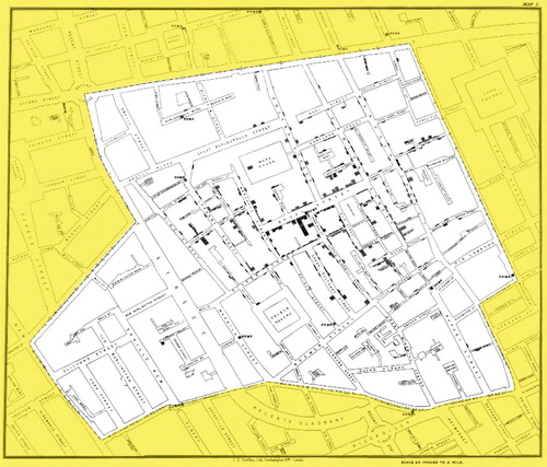
Displaying data on a map is certainly not a new idea. In fact, Dr. John Snow used maps to identify the source of a cholera outbreak in 19th century London. Cholera struck London three times during Snow’s life: in 1832, 1848–49, and 1853–54 (Bynum 2013). The prevailing theory at the time was that cholera was transmitted through the air (Chetwynd and Short 2006). Some believed that the disease was carried on the breath of infected individuals, others blamed the stench from rotting garbage in the densely populated city. The cholera organism was not discovered until 1854 and was not finally accepted as the cause until 1883. But as a trained medical doctor, John Snow had long thought that cholera was transmitted via water contaminated by feces, and he first published this in 1849. To support his theory, Snow used data collected by William Farr at the General Register Office. Snow even took it a step further, visiting the homes of every person who died from cholera in South London, to discover further details about their water source (Hajna, Buckeridge and Hanley 2015). What did he do with all of the data? He plotted it on a map, of course! This allowed him to discover a spatial relationship between the residences of the deceased and the location of public water pumps. The map in Figure 1 is from the UCLA John Snow website, which is very extensive and useful for students and educators (http://www.ph.ucla.edu/epi/snow.html). Snow plotted the address of each cholera death on the map as a short line, which created bars in aggregate (zoom in on the map to see this). Near the center of the map, you cannot help but notice a tall stack of such lines (Frerichs 2001). This cluster of deaths is very close to a particular water pump, the now infamous Broad Street pump. A quick scan of the map, looking for other water pumps, shows no additional clustering of deaths. The Broad Street pump looks very suspicious indeed. But what about the fact that there were relatively few deaths at the nearby brewery and work house? Snow discovered that the work house had its own water pump, and the brewery workers tended to drink beer, so neither had much use for the Broad Street pump. Now all Snow had to do was to convince the authorities to turn off the pump. This was not easy, especially since his theory of cholera being water-borne was still not accepted, and an initial inspection of the pump found everything to be fine. But Snow persisted, and a second inspection confirmed Snow’s suspicion: a leak from a cesspool into the pump shaft (Lai 2011). The pump handle was removed. Not only was the cholera epidemic over in London, but the developed world has been largely free of epidemic cholera ever since (Hill 1955).

Fig. 1 John Snow’s Map 1 (1854). Source: http://www.ph.ucla.edu/epi/snow/snowmap1_1854_lge.htm (a larger version).

Another famous map from history is Charles Minard’s “flow map” of Napoleon’s ill-fated Russia campaign, in which the width of the metaphorical river is proportional to the size of Napoleon’s army. This map was featured in a recent article by Andrews and Wainer (2017), who created similar maps describing the Great Migration of African-Americans from the South following the Civil War in the spirit of W.E.B. DuBois’s work.

The next section outlines the definitions and examples of several types of maps, all of which are examples of thematic maps.

2 Thematic Maps

A thematic map, as the name suggests, is a map of a theme or topic. In contrast to reference maps which show geographic features such as forests, roads, political boundaries, etc., thematic maps emphasize the spatial distribution of one or a small number of variables. They are designed to convey a message to a specific audience which can either be understood at a glance or, in more complex cases, requires more careful examination and analysis. Thematic maps have several variants: we present some of the most common types in the following sections, including choropleth, proportional symbol, dot, multi-type, and bivariate choropleth maps.

2.1 Choropleth Maps

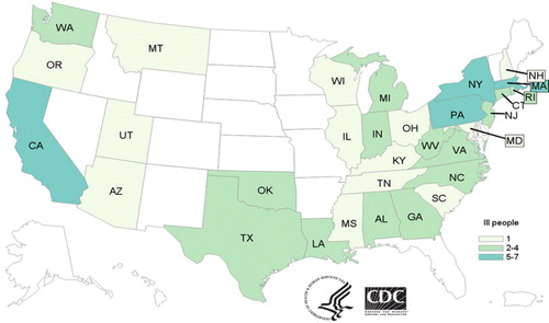
Choropleth maps are used for charting data that are attached to specific areal enumeration units such as countries, states, or counties. To produce a choropleth map, the observations are grouped by areal units and summary statistics are calculated for each. Then the summary statistics are grouped into color groups and the areal units are colored appropriately. Figure 2 displays a choropleth map produced by the Centers for Disease Control and Prevention showing the distribution by state of the incidences of a 2018 outbreak of Salmonella infections linked to Kellogg’s Honey Smacks Cereal. The map highlights that most infections occurred in the Northeast and California.

Fig. 2 Choropleth map that shows the number of people infected with the outbreak strain of Salmonella Mbandaka, by state of residence, as of June 14, 2018. Source: https://www.cdc.gov/salmonella/mbandaka-06-18/map.html.

2.2 Proportional Symbol Maps

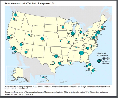
In contrast to the areal locations displayed by choropleth maps, proportional symbol maps (also called graduated symbol maps) represent data associated with point locations—which, for example, would be appropriate for data associated with cities on a nationwide U.S. map. The data are displayed with proportionally sized symbols such that their size in area is proportional to the quantity being represented. This provides a natural visual hierarchy in which the more important features are represented by larger symbols. Figure 3 displays a proportional symbol map from the Department of Transportation that shows the distribution of the number of people boarding a plane at the top 50 U.S. airports in 2015. We can see that ATL, ORD, and LAX are the busiest airports in the continental United States, as their corresponding circles seem to be larger than the 25 million circle in the legend. Note that Snow’s map in Figure 1 is also a proportional symbol map.

Fig. 3 Proportional symbol map showing the number of enplanements at the top 50 U.S. airports in 2015. Source: https://maps.bts.dot.gov/MapGallery/.

2.3 Dot Maps

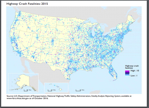
As the name suggests, a dot map (or dot density map) uses dots to show the spatial density pattern of a feature or occurrence. In its simplest form, density is represented by the number of dots per area. Note, though, that a dot is not required to represent a single unit and may indicate any number of entities; for example, one dot might represent 1, 25, or 500 households. Dot maps usually show the spatial distribution of a single variable, although different colored dots could be used to show multiple distributions. Figure 4 shows a dot map from the Department of Transportation of the distribution of U.S. highway crash fatalities in 2015. Notice that different colored dots are used in this map to denote where multiple highway crash fatalities occurred at a single location. As we might expect, the map shows that more highway crash fatalities occur within the areas of the continental United States that are the most heavily populated.

Fig. 4 Dot map showing the locations of U.S. highway crash fatalities in 2015. Source: https://maps.bts.dot.gov/MapGallery/.

2.4 “Multi-Type” Maps

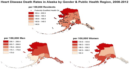
Some maps contain a combination of features from choropleth, proportional symbol, or dot maps. Figure 5 provides a combined choropleth and dot map that uses the choropleth map to display the distribution of heart disease death rates in Alaska by public health region, and the dot map to display the geographic locations of federally qualified health centers. There may be a connection between the northern public health region having the highest death rates (as indicated by the darkest red shading) and having what appears to be the lowest density of qualified health centers (according to the dots).

Fig. 5 Choropleth/dot map that displays the distribution of heart disease death rates in Alaska by gender and public health region between 2008 and 2012. Source: https://www.cdc.gov/dhdsp/maps/gisx/mapgallery/AK_HDGender.html.

2.5 Bivariate Choropleth Maps

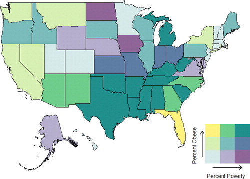
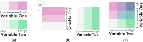
An interesting extension of the choropleth map for a single variable is the bivariate choropleth map. In it, the observations are grouped into classes in terms of their bivariate distribution. The following description borrows from http://www.joshuastevens.net/cartography/make-a-bivariate-choropleth-map/ (Stevens 2015). This bivariate distribution is often displayed as a 3 by 3 array of color shades that combines color “ramps” for each variable (see Brewer 1994). Figure 6 provides an example construction of such an array. Maps with more than 9 classes are generally discouraged.

Fig. 6 Choropleth plot construction: (a) Each variable has a color “ramp”; (b) these two ramps are overlaid on top of each other (picture the Variable One ramp moving to the right on top of the Variable Two ramp); (c) the bivariate distribution of the two variables corresponds to a 3 by 3 array of colors.

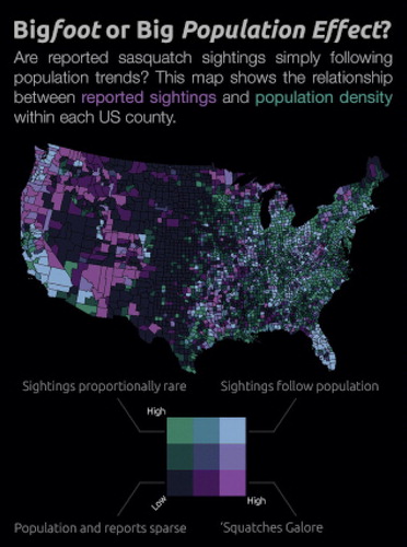
For example, a bivariate choropleth map showing the number of bigfoot sightings and population density for U.S. counties is given in Figure 7. Note that light purple (bottom right in the color array) indicates an area with a large number of bigfoot sightings relative to the sparse population, and light green (top left) indicates an area with a low number of sightings, despite the dense population. Therefore, a general interpretation of the graph is that there are more bigfoot sightings in the western U.S. than in the eastern U.S., though there are regional deviations from this pattern.

Fig. 7 Bivariate choropleth map that displays the relationship between reported sightings of Bigfoot between 1921 and 2013, and population density within each U.S. county. Source: http://www.joshuastevens.net/visualization/squatch-watch-92-years-of-bigfoot-sightings-in-us-and-canada/.

3 Using Maps in the Statistics Classroom

3.1 Integrating Maps Into the Introductory Statistics Course

The topic of maps fits under the umbrella of descriptive statistics. It would likely be discussed after univariate and bivariate numerical/graphical summaries as an extension of the idea of descriptive statistics to multiple variables. We view maps as an important piece in the overall goal of students learning to gain insights from data-based visualizations. Thus, maps should be viewed as a subtopic, not a topic in itself, and should not take more than an additional day (two at most) to discuss. This time can perhaps be found from the time that was traditionally spent reviewing basic statistics, which is mentioned under the section of the GAISE Report “Suggestions for Topics that Might be Omitted from Introductory Statistics Courses.” This section states that “histograms, pie charts, scatterplots, means, and medians are now taught in middle and high school and are a prominent part of the Common Core State Standards” (p. 24). This section also recommends abandoning antiquated practices such as constructing plots by hand and looking up p-values/quantiles on tables and placing less emphasis on probability theory in introductory statistics courses.

In the rest of this section, we present an example of an introductory data exploration based upon a choropleth map. The following contains a description of the activity. For your convenience, we include a ready-to-use version of the activity in Appendix B.

3.2 Introducing the Activity

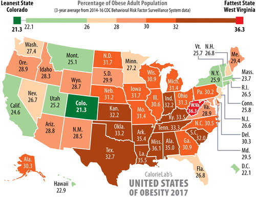
The activity “United States of Obesity” has students explore the relationship between two variables. The first variable is percentage of obese adults in the United States, based upon 3-year averages from 2014 to 2016. We ask students to refer to the “United States of Obesity” map shown in Figure 8. The second variable is percentage of people living in poverty in the United States, also based on 3-year averages from 2014 to 2016.

Fig. 8 Choropleth map that shows the distribution of the percentage of the obese adult population in each state based upon 3 year averages from 2014 to 2016. Source: http://calorielab.com/news/wp-images/post-images/fattest-states-2017-big.jpg.

Students are introduced to a choropleth map and learn how such a map can be used to display data. Using the data from a choropleth map along with additional data, students will explore the relationship between obesity and poverty within the United States. Students will gain experience creating a scatterplot, interpreting the strength of the linear relationship through the correlation coefficient, and fitting a simple linear regression equation using the software plotly. Further, students will create their own univariate choropleth maps using plotly and interpret the results from the activity in the context of the problem. (Please see Appendix C.1 for step-by-step instructions on using plotly.) Finally, students will be presented with a bivariate choropleth map and will be asked to interpret the map (see Appendix C.2).

To complete this activity, students should be able to summarize and analyze univariate data, they should be comfortable using a computer, and they will need an E-mail address. Students should also have a basic understanding of concepts such as scatterplots, best-fit lines, and correlation. They will need a calculator, pencil, and a computer with internet access.

For this activity to be completed entirely in the classroom, two class periods will be needed. However, if a few questions are to be assigned outside of class, then only one class period is required. The instructor will provide the Activity Worksheet (Appendix A) and the Excel data file, available at facweb.gvsu.edu/adriand1/United_States_of_Obesity.xlsx. Please also see Malloure et al. (2013) for an earlier version of this activity with less emphasis on maps.

3.3 Describing the Activity

Before delving into the activity, ask your students how they would go about representing obesity data for each of the 50 states. This will start a discussion about various methods that the students might have already learned before introducing them to thematic maps. Explain that a thematic map is used to show themes or topics on a map, using the United States of Obesity 2017 map as an example. A choropleth map is a specific example of a thematic map, in that a summary statistic is gathered for specific areas and then each area is shaded in a color representing the magnitude of the statistic. In the United States of Obesity 2017 map, each state is an area and the color scale goes from green to red with the darkest green representing the lowest percentage of obesity and the darkest red representing the highest percentage of obesity. Stress to students the importance of using a statistic like the mean, median, or percentage instead of a raw count for a choropleth map. If raw counts are used, then the population in each state will essentially drive the colors instead of the real information of interest. With this better understanding of the choropleth map, explain to students the goal of the activity.

Two of the most common concerns in the United States of late are poverty and obesity. Data have been collected on the 3-year, 2014 through 2016, average poverty rate and obesity rate in all 50 states and D.C. In this activity, students determine if the poverty rate is related to the obesity rate within each state. More specifically, can the poverty rate be used to predict the obesity rate in a given state?

The data for this activity are presented in a table on the last page of the Activity Worksheet.

A copy of the data table appears in Table 1.

Table 1 Poverty rate and obesity rate by state.

State	Poverty rate	Obesity rate	State	Poverty rate	Obesity rate
Alabama	18.30	35.00	Missouri	14.77	31.40
Alaska	10.47	30.30	Montana	14.43	25.10
Arizona	17.33	28.80	Nebraska	12.13	31.20
Arkansas	18.40	35.40	Nevada	14.57	26.70
California	15.33	24.60	New Hampshire	8.23	26.80
Colorado	11.50	21.30	New Jersey	10.77	26.60
Connecticut	10.37	25.80	New Mexico	20.50	28.50
Delaware	12.20	30.30	New York	15.33	25.90
District of Columbia	17.87	22.10	North Carolina	16.33	30.50
Florida	15.63	26.80	North Dakota	11.07	31.70
Georgia	17.10	30.90	Ohio	15.07	31.30
Hawaii	10.43	22.90	Oklahoma	16.33	33.20
Idaho	14.77	28.30	Oregon	15.10	28.90
Illinois	13.67	30.60	Pennsylvania	13.23	30.20
Indiana	14.60	32.20	Rhode Island	13.67	26.50
Iowa	12.07	31.70	South Carolina	16.63	32.00
Kansas	12.90	32.20	South Dakota	13.73	29.90
Kentucky	18.70	33.50	Tennessee	16.93	33.30
Louisiana	19.87	35.50	Texas	16.23	32.70
Maine	13.33	29.40	Utah	11.07	25.20
Maryland	9.83	29.50	Vermont	11.43	25.70
Massachusetts	11.17	23.70	Virginia	11.33	28.90
Michigan	15.67	31.40	Washington	12.23	27.40
Minnesota	10.53	27.20	West Virginia	18.03	36.30
Mississippi	21.43	36.10	Wisconsin	12.37	30.90
			Wyoming	11.20	28.70

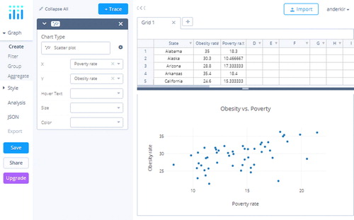
The first step in the activity is to introduce students to the plotly website and have them create their free account. Once this is done, have students construct a scatterplot with the poverty rate on the x-axis and the obesity rate on the y-axis. In the final plot, there should be 51 points representing the 50 states and Washington D.C. with both axes labeled appropriately. Refer to Appendix C for instructions to create a scatterplot in plotly.

Once the plot is finished, students are asked to comment on the relationship between poverty rate and obesity rate. Students should comment on three aspects of this plot: strength, direction, and form (linear, exponential, polynomial, etc.). In this scenario, the relationship between poverty rate and obesity rate appears to be of medium strength, positive, and linear.

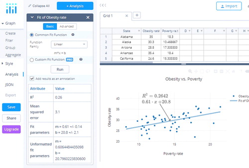
To obtain a quantitative value of this relationship, students generate the regression equation using plotly. They will be able to add the line to the scatterplot and have the equation appear on the plot (this display will include R²). Refer to Appendix C for instructions to add these items to the plot. Students will need to take the square root of R² = 0.2642 using their calculators. The value of the correlation coefficient is r = 0.541. Students should know the possible values of r are between –1 and 1 and the farther from 0, the stronger the linear relationship. When students interpret r = 0.541 in the context of the problem, it should be similar to what they said when they interpreted the scatterplot. There is a medium strength, positive, linear relationship between state poverty rates and obesity rates averaged from 2014 to 2016.

The estimated regression equation is: $\widehat{\text{Obesity}}=0.61(\text{Poverty})+20.8$. After students add this equation to their scatterplot, it should resemble the plot in Figure C3. From the estimated regression equation, students interpret both the slope and intercept values in the context of the problem. The slope interpretation should say something similar to, “for every increase of 1 percentage point in the poverty rate, we can expect the obesity rate to increase by 0.61 percentage points.” As for the interpretation of the intercept term, students should understand that it corresponds to the case where the poverty rate is 0, so the interpretation should read, “when the poverty rate is 0, we expect the obesity rate to be 20.8%.” Even though students are asked to interpret this value as an exercise in the Activity Worksheet, they need to understand that it should not be interpreted in a real-life example. There are no data points even close to a 0 percent poverty rate, so there are no values supporting the claim that at this point the expected obesity rate is near 21%. Also, in reality, there will never be a state with a poverty rate of 0, so in this regression equation, the y-intercept is simply present to improve the fit of the regression equation.

Students are asked to look at their scatterplot and try to determine if any states appear to be pulling the regression line in a certain direction. From the scatterplot it does appear that the slope of the line is being pulled down, due to the two points at (17.87, 22.10) and (20.50, 28.50). These points correspond to the District of Columbia and New Mexico, respectively.

In regression, extrapolation of the regression equation to points outside the range of the collected values of the independent variable should never be done. According to the Census Bureau, the poverty rate for Puerto Rico was 46.2% in 2014 (https://www.puertoricoreport.com/u-s-census-data-show-continued-decline-puerto-ricos-population/#.WqvH5GrwZhE). If 46.2% were a valid value to use in the regression equation, students would see that $\widehat{\text{Obesity}}=0.61(46.2)+20.8=48.98$; and the obesity percentage in Puerto Rico would be estimated to be 48.98%. In terms of the actual use of this prediction, students should adamantly refuse to use it in a real-life scenario. There are no data points providing information to the regression equation anywhere near a poverty rate of 46.2%. There is no evidence to suggest that the linear relationship will continue past the last poverty rate in the dataset. In fact, according to 2016 data collected through the Behavioral Risk Factor Surveillance System (BRFSS), 30.7% of adults in Puerto Rico are obese (https://www.cdc.gov/obesity/data/prevalence-maps.html), showing that the extrapolated estimate of 48.98% is very far off the mark.

Throughout the activity, students have been asked to provide interpretations of the parameter estimates of the model and the correlation coefficient. One important remaining question asks students if the regression equation implies that poverty rate directly causes the increased obesity rate in states across the United States. Clearly, students should understand that correlation between the two variables in no way implies causation. This study was purely observational, so students were simply asked to determine if there was a relationship between poverty and obesity. This does not determine that poverty leads to obesity. To check for causation, an experiment would have been needed. An experiment would randomly divide subjects of similar characteristics into two groups, with one living a period of time in severe poverty while the other was living a comfortable lifestyle. Over the course of the experiment, the obesity rates in the two groups could be compared to determine if the obesity rate is significantly higher when living in poverty. Not only would this be unethical, but also nearly impossible to carry out. The only main difference between the two subject groups would have to be the income/lifestyle characteristic. Many confounding variables will play a role in the experiment. Therefore, students should understand that even though poverty and obesity are related, it cannot be concluded that poverty causes obesity.

In the activity, students found that District of Columbia and New Mexico appear to be influencing the regression equation. If you have time, ask students to explore how the regression equation changes if both of the points are removed, and how this differs from just having one of the points removed. This will illustrate the influence of outliers.

The activity goes on to guide students in the creation of two univariate choropleth maps using plotly. The obesity map created in plotly uses the color red for high obesity rates, indicating West Virginia (36.3%), Mississippi (36.1%), Louisiana (35.5%), Arkansas (35.4%), and Alabama (35.0%) as the states with the five highest obesity rates. Similarly, the poverty map created in plotly uses the color red for high poverty rates, indicating Mississippi (21.4%), New Mexico (20.5%), Louisiana (19.9%), Kentucky (18.7%), and Arkansas (18.4%) as the states with the five highest poverty rates. Answers will vary, but students might point out that Mississippi, Louisiana, and Arkansas have high rates for both obesity and poverty.

Finally, the activity presents students with a bivariate choropleth map. This map makes it much easier to see which states have high (or low) obesity and poverty rates, or some other interesting combination, such as low poverty and high obesity. We recommend showing your students Figure C10, since this makes a solid connection between the scatterplot and the color grid, making the map much easier to grasp. You might also want to show your students the animation at http://www.joshuastevens.net/cartography/make-a-bivariate-choropleth-map/ which shows the two color schemes, one for each variable, being superimposed on top of each other, resulting in a 3 × 3 grid of 9 colors.

Students are asked which states have high obesity and poverty rates, and the top right color (teal) indicates Texas, Oklahoma, Arkansas, Louisiana, Mississippi, Tennessee, Alabama, Kentucky, West Virginia, South Carolina, and Michigan as the states with the highest obesity and poverty rates in combination. This does not perfectly match up with the states that stand out solely for high obesity rates or solely for high poverty rates, so students might ponder this. Many states, such as Mississippi, Louisiana, and Arkansas stand out on both univariate choropleth maps as well as the bivariate map, but some other states, such as Texas and Michigan, only stand out on the bivariate map due to their combination of relatively high obesity and poverty rates.

Students are asked to relate what they see in the bivariate map to the scatterplot. They might say that the two states that appear in the upper right corner of the scatterplot, thus meaning that they have both high obesity and high poverty rates, are Mississippi and Louisiana. These two states appear as teal, the upper right color in the grid.

Specifically, they are asked to focus on Colorado, since it appears as an outlier in the lower left corner of the scatterplot, corresponding to a low/low combination of obesity and poverty rates. Students should make the connection and see that on the map, Colorado appears in light blue, which is the color occupying the lower left corner of the grid.

4 Conclusions

Maps are frequently used to display data distributions that have a geographic context. They are commonly seen on web pages, in newspapers, magazines, and on TV newscasts. Arguably, it may be stated that maps appear as commonly in today’s media as data displays typically discussed in an introductory statistics course, such as pie charts and bar graphs. We propose the use and interpretation of statistical maps in an introductory course.

In particular, univariate choropleth maps are very commonly seen in the media. The distributions of many variables of interest for the 50 U.S. States are displayed with choropleth maps. An extension of a univariate choropleth map is the bivariate choropleth map. In it, the observations are grouped into classes in terms of their bivariate distribution. The bivariate distribution is often displayed as a 3 by 3 array of color shades that combines color “ramps” for each variable.

In our activity, we ask students to interpret a univariate choropleth map and then use plotly to construct two univariate choropleth maps. After an introduction to bivariate choropleth maps and their interpretation, we ask students to think about how what the map shows about the relationship between the two variables coincides with what a scatterplot shows about the relationship between the two variables.

Appendix A: Biases in Election Maps

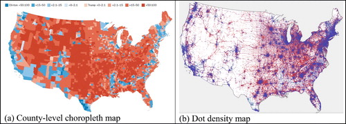
It is well-known that standard maps of U.S. Presidential election results can be visually misleading (National Geographic; October 12, 2016). For example, the county-level choropleth map of the 2016 election results (see Figure A1(a)) “grossly exaggerates the extent of [Donald] Trump’s victory” (TIME; May 17, 2017) because Trump won the “vast majority of U.S. counties” (2649 to 503), which tended to have smaller populations and be geographically larger than average than the counties Hillary Clinton won. The visual impression is that Trump won by a landslide because “Trump’s territory accounts for 75.6% of the nation’s landmass.” In fact, The New York Times (May 13, 2017) reports that “Trump keeps a stack of [such] color-coded maps” in his office, “sometimes hands the maps out to visitors as a kind of parting gift,” and “dwells on the map” in conversations. A less misleading map is the dasymetric dot density map by Kenneth Field shown in Figure A1(b). It is constructed so 1 dot stands for 1 vote (red for Trump, blue for Clinton), and so the density of the dots is much greater in urban areas than rural areas, a feature missed by the standard choropleth map. The visual impact “does not distort the visual weight of the relative proportions of red and blue simply by virtue of the size of a geographical area,” as Field states in his description of the map technique.

Fig. A1 Maps of 2016 U.S. presidential election results: (a) county-level choropleth map; (b) dot density map. Sources: (a) https://www.washingtonpost.com/news/politics/wp/2018/07/30/presenting-the-least-misleading-map-of-the-2016-election/; (b) http://arcg.is/1yLmOL.

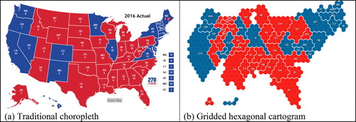
Of course, U.S. Presidents are not elected based on number of votes but rather by the number of electors in the Electoral College. The traditional choropleth electoral map shown in Figure A2(a) suffers from the same bias described above: the Great Plains/Mountain states with large areas and sparse population density are visually weighted disproportionally compared to northeastern states with small areas and larger population density. The gridded hexagonal cartogram in Figure A2(b) corrects this bias. In it, one electoral vote is represented by one hexagon of area so there is no visual bias (though, of course, the geography is distorted). The cartogram, a term whose first use is credited to Charles Minard (of the flow map of Napolean’s campaign), can be defined as “a diagrammatic map type that represents the mapped area by distorting the geometry of the feature itself” (Field 2017).

Fig. A2 Electoral Maps of 2016 U.S. presidential election: (a) traditional choropleth; (b) gridded hexagonal cartogram. Sources: (a) https://www.270towin.com/2016_Election/interactive_map; (b) https://gistbok.ucgis.org/bok-topics/2018-quarter-02/cartograms.

Appendix B: Classroom Activity

In this activity, you will use simple linear regression and choropleth maps to explore the relationship between poverty and obesity in the United States between 2014 and 2016. You will use a free online graphing tool called plotly to create graphs and compute statistics. The data (Table 1) are saved in an Excel file for you to use. You will answer several questions as you work through this activity.

1. Before starting your computer work, look at the United States of Obesity 2017 map. Use the legend at the top of the map to see how the color spectrum corresponds to obesity rate. What is the value and color for the state you live in? How many states have a lower obesity rate? How many states have a higher obesity rate?

   Create a free account on the plotly website and make a scatterplot with each state’s obesity rate on the vertical axis and each state’s corresponding poverty rate on the horizontal axis. To do this, go to https://plot.ly/ and enter your E-mail address. Choose a username and password. After clicking on a link in an E-mail plotly will send you, you can log in. Next, click on the Import button and choose the Excel dataset containing the obesity and poverty data for the U.S. Notice that variable names occupy the first row. Click the arrow by Column 0 and select Rename header, then type in State. Repeat for the remaining columns. Delete the first row by selecting it, then right-click near the “1” and select Remove selected rows. Now for the scatterplot: Note that the default Chart Type (left side of screen) is scatterplot. We want to use poverty rate to predict obesity rate, so we will denote X = poverty and Y = obesity. Click on the drop down arrow for X and choose poverty rate; click on the arrow for Y and choose obesity rate. This creates the scatterplot. The graph is interactive—if you hover your mouse pointer over a point, it will give the X and Y values. Pull down the Hover Text arrow and choose State. Now the state name will also appear.

2. From the scatterplot alone, interpret the relationship between poverty and obesity.

   Add the regression line to the scatterplot. Click Analysis, then click the blue + Analysis button. Select Curve fitting. For Target Trace, choose Obesity rate. The default will be a Linear fit, so click Run. This will add the line to the plot. Select Add results as an annotation. This will superimpose the equation of the line and the R² value on the graph.

3. Calculate the numerical value of r, the correlation coefficient between state obesity rates and state poverty rates. (Remember that r can be computed by taking the square root of R². If the direction of the relationship is negative, you will have to put a negative sign in front of r.) Does the value support your interpretation in question 2? Explain.

4. Write the estimated regression equation for predicting a state’s obesity rate from the state’s poverty rate.

5. Interpret the slope of the estimated regression equation in the context of this problem.

6. Interpret the intercept of the estimated regression equation in the context of this problem. Practically speaking, is it reasonable to interpret this intercept value? Why or why not?

7. Based on the regression equation and scatterplot, are there any states that appear to be “pulling” the line in one direction or the other? If so, which states are they, and in what direction do they appear to be pulling the line?

8. According to the Census Bureau, in 2014 Puerto Rico had a poverty rate of 46.2%. Suppose Puerto Rico became a state. Use the regression equation found in question 2 to predict the obesity rate for Puerto Rico.

9. Is it okay to extrapolate the regression equation to include Puerto Rico? That is, is it reasonable to apply the regression equation to predict the obesity rate for Puerto Rico?

10. From this simple linear regression analysis, can you conclude that an increase in the poverty rate directly causes the obesity rate to increase? Why or why not?

    Now you will create your own maps using plotly. You will create two maps, one with obesity rates and one with poverty rates. At the top right of the screen, hover over your username and select New Chart. This will create a new tab with a blank data grid. Hover over your username again and select My Files. Look for the data file name you saved and click the Edit button. Once the data are again in view, we need to change the chart type to choropleth map. Click in the box under Chart Type. From the collection of chart types that pops up, pick the Choropleth Map in the upper right. A blank map of the world will initially appear. Next, we specify what information we are using in the map. The locations must be given by state abbreviations, so we need to create another column. Click on the down arrow for the State column in the data grid and choose Add state name abbreviation. A new column of state abbreviations will appear. Rename this column header if you like. Select the new column of state abbreviations for Locations, and select obesity rate for Values. Choose USA State Abbreviations for Location Format, and USA for Map Region. There is only one option for Projection associated with the USA Map Region, Albers USA, which will be automatically selected.

    By default, plotly creates maps with a sequential color scheme. To make your map look more like the original United States of Obesity map, you can change it to use a diverging color scheme. Click on the Style heading in the far left-hand bar, which will display several options, the first two of which are Traces and Layout. Traces control the color scale. The second-from-left color scale is an example of a diverging scheme. Click on this color scheme and notice how the map changes. You may also want to increase the resolution of the map under the Geo Layout settings. You will roughly increase the map resolution by a factor of two when you change the resolution from the default of 1:110,000,000 to 1:50,000,000. Do not forget to save your map by using the Save button on the left bar. If you want to easily share your creation with others, click the Share button. This will give you a web address so anyone can view your graphs.

    Once you are finished creating a choropleth map showing U.S. obesity rates, follow the directions again to create a choropleth map showing U.S. poverty rates.

11. Now that you have maps showing obesity and poverty rates for the United States, study them to see what else can be learned. Which states have high poverty rates and high obesity rates?

    The maps you just created in plotly are called univariate choropleth maps, since they only showed one variable at a time, either obesity rate or poverty rate. Bivariate choropleth maps show two variables at a time, using a combination of colors in a 3 × 3 grid. Unfortunately, bivariate choropleth maps cannot be created in plotly, but one is provided for you to interpret. As you look at the map, pay close attention to the color grid and note that states with high rates for both poverty and obesity appear as a teal color, while states with low rates for both poverty and obesity appear as light blue. Yellow indicates states with low poverty and high obesity rates, purple indicates states with high poverty and low obesity rates, and so on.

12. According to the bivariate choropleth map, which states have high poverty rates and high obesity rates? Relate this back to the scatterplot. Find an interesting point on the scatterplot, perhaps an outlier like Colorado. How does this state appear on the bivariate map?

Univariate Choropleth Map Showing Obesity Rates by State

Bivariate Choropleth Map Showing the Relationship Between Poverty Rate and Obesity Rate

Appendix C: Examples of Using Software to Make Maps

C.1 Making Scatterplots and Maps With Plotly

Choropleth maps can be created with a variety of software packages, such as Microsoft Excel, Google Sheets, R, and SAS. In this article, we will demonstrate how to use the free online application plotly, which contains a good combination of simplicity along with a moderate amount of customizability. An added bonus is that graphs created in plotly can be freely shared on the web. Plotly has a variety of products for sale, but we will utilize their free website called Graph Maker at https://plot.ly/create/. (The help article at https://help.plot.ly/excel/choropleth-maps/ was a starting point for us.) To use this software, it is first necessary to create an online account. Simply enter your E-mail address, and choose a username and password. After clicking on a link in an E-mail plotly will send you, you can log in.

We demonstrate how to perform a simple linear regression analysis and create a choropleth map for the “United States of Obesity” data, as in the activity in Section 3.

C.1.1 Data Import

Begin by clicking on the Import button and choose the Excel dataset containing the obesity and poverty data for the United States. A link that will take you to the Excel dataset is http://facweb.gvsu.edu/adriand1/United_States_of_Obesity.xlsx. After closing the empty Grid tabs, your screen should look like Figure C1.

Fig. C1  Screen shot of the plotly Graph Maker interface after the data is imported.

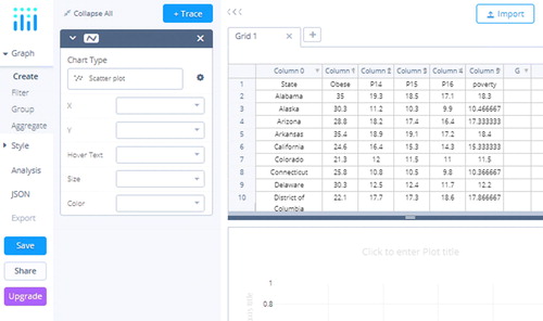
Notice that variable names occupy the first row. Click the arrow by Column 0 and select Rename header; then type in State. Repeat for the remaining columns. Delete the first row by selecting it, then right-click near the 1, and select Remove selected rows. Note that the Poverty rate column is the average of the years 2014–2016. Thus, you may delete the P14–P16 columns if you like by clicking the down arow for the column and choosing Remove selected columns.

C.1.2 Scatterplot

Note that the default Chart Type on the left side of the screen is scatterplot. In the activity, students are asked to use poverty rate to predict obesity rate, so X = poverty and Y = obesity. This creates the scatterplot which is shown in Figure C2. Note the gray text: Click to enter Plot title.

Fig. C2 Screen shot of the plotly Graph Maker interface after the scatterplot is created.

If we wished to include a third variable, we could use the Size or Color functions to add further dimensions to the plot. The graph is interactive: if you hover your mouse pointer over a point, it will give the X and Y values. Pull down the Hover Text arrow and choose State. Now the state name will also appear.

C.1.3 Regression Line

Let’s add the regression line to the plot. Click Analysis, then click the blue + Analysis button. Select Curve fitting. For Target Trace, choose Obesity rate. The default will be a Linear fit, so click Run. This will add the line to the plot. Select Add results as an annotation. This will superimpose the equation of the line and the R² value on the graph as shown in Figure C3. You may want to adjust the position of this by dragging it.

Fig. C3 Screen shot of the scatterplot with the regression line added.

C.1.4 Saving Your Work

At this point, you will want to save your plotly work. Click the blue Save button on the left. Note that you will be able to save the data grid and the scatterplot, giving your own names for each. When using the free Graph Maker, you are required to save your graphs as public: they will be freely viewable by the public.

C.1.5 Univariate Choropleth Maps

Now we can create choropleth maps showing the data on a map of the United States. We will create two univariate choropleth maps, one with the obesity rates and one with poverty rates.

At the top right of the screen, hover over your username and select New Chart. This will create a new tab with a blank data grid. Hover over your username again and select My Files. Look for the data file name you just saved and click the Edit button. Once the data are again in view, we need to change the chart type to choropleth map. Click in the box under Chart Type that contains the words scatterplot. From the collection of chart types that pops up in the dialog box shown in Figure C4, pick the Choropleth Map in the upper right. A blank map of the world will initially appear.

Fig. C4 Screen shot of the dialog box for creating a choropleth map. The choropleth map in the upper-right is selected, and variables are filled in on the right-hand side.

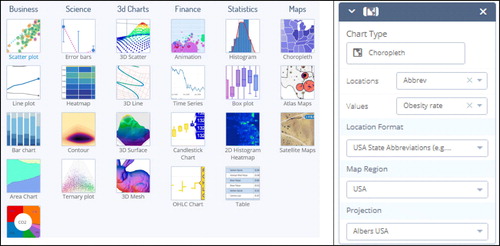
Next, we specify which columns in the dataset represent the locations and the values in the choropleth map dialog box on the right-hand side in Figure C4. The locations must be given by state abbreviations, so we need to create another column. Click on the down arrow for the State column in the data grid, and choose Add state name abbreviation. A new column of state abbreviations will appear. Rename this column header if you like. Select the new column of state abbreviations for Locations, and select Obesity rate for Values. Choose USA State Abbreviations for Location Format and USA for Map Region.

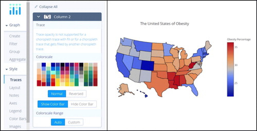
Completing the above will produce the map shown in Figure C5(a). You can create a title for the plot by clicking on the gray text Click to enter Plot title and typing your title. You can also make a label for the color bar on the right by clicking on the gray text near the top of the bar. We will use the title “The United States of Obesity” and the label “Obesity Percentage.” The result is shown in Figure C5(b).

Fig. C5 Default plotly choropleth map (a) before and (b) after adding the title and label.

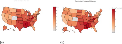
We can modify some of the display options by clicking on the Style heading in the far left-hand bar (see Figure C6(a)), which will display several options, the first two of which are Traces and Layout. Traces controls the color scale using the dialog box shown in Figure C6(a). The default color scale is shown on the left, and others can be chosen by clicking on the different color bars. Overall, color schemes for representing quantitative variables on choropleth maps can be divided into sequential and diverging schemes. There are also schemes designed for categorical variables, but we will not discuss those here. As described by http://colorbrewer2.org/learnmore/schemes_full.html, “lightness steps dominate the look” of sequential schemes, with light colors for low data values to dark colors for high data values. For example, the default color scheme in plotly is sequential. In contrast, diverging schemes “put equal emphasis on mid-range critical values and extremes at both ends of the data range. The critical class or break in the middle of the legend is emphasized with light colors, and low and high extremes are emphasized with dark colors that have contrasting hues” (http://colorbrewer2.org/learnmore/schemes_full.html). The second-from-left color scale used in Figure C6 is an example of a diverging scheme, as is the one used in the original map in Figure 8. Click on this color scheme and notice how the map changes. Diverging color schemes are ideally suited for variables with negative and positive values. However, they can also provide more definition to a color scale, as well as clearer information about whether particular values are above or below the middle. The diverging scheme in Figure C6 seems to be more descriptive than the sequential scheme in Figure C5. For instance, it is easier to tell that the states of Florida and Minnesota have below average obesity percentages, in contrast to their neighboring states.

Fig. C6 Screen shot for changing the color scale.

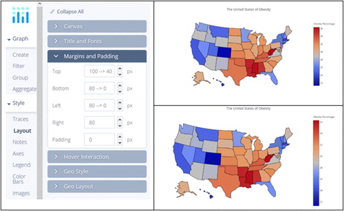
Next, we will change two options within the Layout category. First, because the default margins are quite generous, we reduce them in the Margins and Padding settings shown in Figure C7. This gives us a larger picture of the map and a longer color bar.

Fig. C7 Screen shot for changing the margins, including before and after maps.

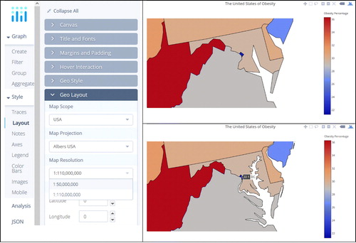
The second task is to increase the resolution of the map under the Geo Layout settings. We will roughly increase the map resolution by a factor of two in changing the resolution from the default of 1:110,000,000 to 1:50,000,000, as shown in Figure C8. This is more noticeable when we zoom in on a portion of the map, as we do in showing the greater Washington, DC region in Figure C8. This can be done with the plus/minus controls in the upper right of the graph area; note that these are not visible until you hover your mouse over them. Another nice interactive feature of the plotly map is that the exact value for an individual state can be queried by hovering your cursor over the state. For example, the obesity percentage of 22.1% in Washington, DC is shown in the bottom graph in Figure C8.

Fig. C8 Screen shot showing changing the resolution, including before and after maps.

C.1.6 The Plotly Dashboard

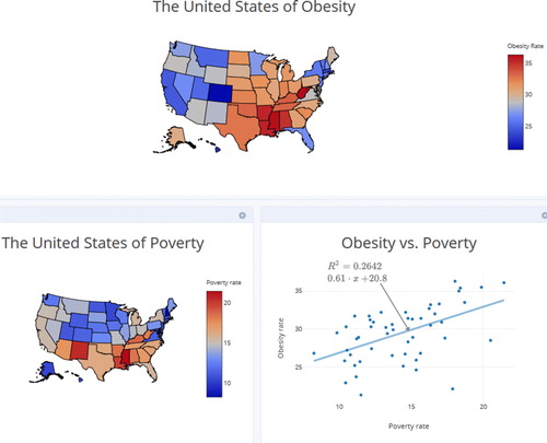
Another nice feature of plotly is that you can create a “dashboard,” a collection of graphs in the same place, often called an infographic. We can gather all of the graphs created so far and arrange them in one image, like a poster. Under your username, select New Dashboard. Under “Get started by adding a:” click the Plot button. Click the Your Files button, and choose any of the graphs you have created. To add a second graph, click the + Plot button at the bottom of the screen. Continue to do this until you have them all in view, and rearrange them (by dragging) until you are happy with the result. The dashboard created for the obesity and poverty data is shown in Figure C9. Then you can Save your dashboard by clicking the blue button at the bottom of the screen. You may also click the Share button, which provides you with a Shareable Link, a web address that’s lets others enjoy the same interactive features (i.e., zooming, panning, querying, etc.).

Fig. C9 The plotly dashboard.

Do not forget to save your map by using the Save button on the left bar, as shown in Figure C3.

Once you are finished creating a choropleth map showing U.S. obesity rates, follow the directions again to create a choropleth map showing U.S. poverty rates.

Unfortunately, it does not appear that bivariate choropleth maps can be created in plotly, so in the next section we will focus on the interpretation of a bivariate choropleth map created in R.

C.2 A Bivariate Choropleth Map for the Obesity and Poverty Data

We will show a bivariate choropleth map for the state-wise poverty and obesity rate data used in the last section as an additional example of a bivariate choropleth map and for practice on its interpretation. These graphics were produced in R with help from http://lenkiefer.com/2017/04/24/bivariate-map/. Figure C10 shows the legend for the bivariate map and the corresponding scatterplot. This is the same scatterplot shown in Figure C2, except that the points (states) are divided into the nine regions of the legend. The two vertical and horizontal lines are terciles; that is, they split the obesity and poverty rates for the states into thirds. Note from the scatterplot that points (or states) representing different colors (in the map) need not be far apart.

Fig. C10 Legend and corresponding scatterplot for obesity and poverty rates.

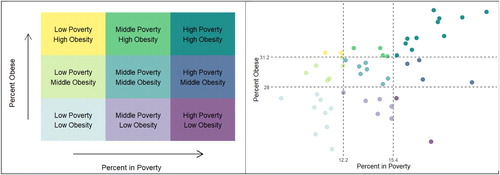
Figure C11 shows the bivariate choropleth map. The most compelling pattern is the group of (high poverty, high obesity) states stretching across the southern U.S. from Texas to West Virginia. There is also a cluster of (low poverty, low obesity) states in the New England region, but it is less noticeable due to the smaller sizes of those states.

Fig. C11 Bivariate choropleth map for the percent obese/poverty data.

References

- Steen, L. ed. (2001), Mathematics and Democracy: The Case for Quantitative Literacy, Princeton, NJ: National Council of Education and the Disciplines.
- Bloch, M., Buchanan, L., Katz, J., and Quealy, K. (2018, July 25). “An Extremely Detailed Map of the 2016 Election,” The New York Times, available at https://www.nytimes.com/interactive/2018/upshot/election-2016-voting-precinct-maps.html.
- GAISE College Report ASA Revision Committee (2016), “Guidelines for Assessment and Instruction in Statistics Education (GAISE) College Report 2016,” available at http://www.amstat.org/education/gaise.
- Giratikanon, T., Katz, J., Leonhardt, D., and Quealy, K. (2014, April 24), “Up Close on Baseball’s Borders,” The New York Times, available at https://www.nytimes.com/interactive/2014/04/23/upshot/24-upshot-baseball.html.
- Hartenian, E., and Horton, N. (2015), “Rail Trails and Property Values: Is There an Association?,” Journal of Statistics Education, 23(2). DOI: 10.1080/10691898.2015.11889735.
- Katz, J. (2016, December 27). “‘Duck Dynasty’ vs. ‘Modern Family’: 50 Maps of the U.S. Cultural Divide,” The New York Times, available at https://www.nytimes.com/interactive/2016/12/26/upshot/duck-dynasty-vs-modern-family-television-maps.html.
- Kapitula, L., and Stephenson, P. (2014), “How Wet Is the Earth?,” STatistics Education Web, available at https://doi.org/https://www.amstat.org/asa/files/pdfs/stew/HowWetistheEarth.pdf.
- Rosling, H. “Gapminder,” available at www.gapminder.org.
- Stoudt, S., Cao, Y., Udwin, D., and Horton, N. J. (2014), “What Percent of the Continental US Is Within One Mile of a Road?,” STatistics Education Web, available at http://www.amstat.org/education/stew/pdfs/PercentWithinMileofRoad.pdf.
- Arms sales: https://www.visualcapitalist.com/arms-sales-usa-vs-russia-1950-2017/.
- Foreign aid: https://www.economist.com/graphic-detail/2016/08/10/where-does-foreign-aid-go?fsrc=scn/fb/te/bl/ed/.
- Human population growth: https://doi.org/https://aeon.co/videos/how-we-became-more-than-7-billion-humanitys-population-explosion-visualised.
- PFAS contamination sites: https://doi.org/https://www.ewg.org/interactive-maps/2019_pfas_contamination/map.
- References for Background on John Snow
- Andrews, R. J., and Wainer, H. (2017), “The Great Migration: A Graphics Novel,” Significance, 14, 14–19. DOI: 10.1111/j.1740-9713.2017.01070.x.
- Bynum, W. (2013), “On the Mode of Communication of Cholera: W.F. Bynum Reassesses the Work of John Snow, the Victorian ‘Cholera Cartographer’,” Nature, 495, 169–170.
- Chetwynd, A., and Short, H. (2006), “Cholera—A Step Too Farr,” Significance, 3, 88–90.
- Frerichs, R. (2001), “History, Maps and the Internet: UCLA’s John Snow Site,” SoC Bulletin, 34, 3–7.
- Hajna, S., Buckeridge, D., and Hanley, J. (2015), “Substantiating the Impact of John Snow’s Contributions Using Data Deleted During the 1936 Reprinting of His Original Essay on the Mode of Communication of Cholera,” International Journal of Epidemiology, 44, 1794–1799.
- Hill, A. (1955), “Snow—An Appreciation,” Proceedings of the Royal Society of Medicine, 48, 1004–1007. DOI: 10.1177/003591575504801204.
- Lai, A. (2011), “London Cholera and the Blind-Spot of an Epidemiology Theory,” Significance, 8, 82–85.
- UCLA John Snow Website: https://doi.org/http://www.ph.ucla.edu/epi/snow.html.
- https://doi.org/http://chnm.gmu.edu/worldhistorysources/unpacking/mapsmain.html.
- https://doi.org/http://en.wikipedia.org/wiki/Thematic_map.
- https://doi.org/http://www.fes.uwaterloo.ca/crs/geog165/maps.htm.
- https://doi.org/http://en.wikipedia.org/wiki/Geographic_information_system.
- https://doi.org/http://en.wikipedia.org/wiki/Map_making.
- http://www.phil.uni-passau.de/histhw/tutcarto/english/index-frames-en.html.
- https://doi.org/http://www.ncjrs.gov/html/nij/mapping/.
- Brewer, C. (1994), “Color Use Guidelines for Mapping and Visualization,” in Visualization in Modern Cartography, eds. A. MacEachren and D. Taylor, Tarrytown, NY: Elsevier Science, pp. 123–147.
- Stevens, J. (2015, February 18), “Bivariate Choropleth Maps: A How-to Guide” [Blog Post], available at http://www.joshuastevens.net/cartography/make-a-bivariate-choropleth-map/.
- Field, K. (2017), “Cartograms,” The Geographic Information Science & Technology Body of Knowledge (3rd quarter 2017 edition), ed. J. P. Wilson, Ithaca, NY: University Consortium for Geographic Information Science. DOI: 10.22224/gistbok/2017.3.8.
- https://doi.org/https://www.nationalgeographic.com/news/2016/10/improved-election-map-cartograms/.
- https://time.com/4780991/donald-trump-election-map-white-house/.
- https://www.nytimes.com/2017/05/13/us/politics/election-is-over-but-trump-still-cant-seem-to-get-past-it.html?_r=0.
- http://carto.maps.arcgis.com/apps/webappviewer/index.html?id=8732c91ba7a14d818cd26b776250d2c3.
- https://doi.org/https://www.270towin.com/2016_Election/interactive_map.
- Malloure, M., Richardson, M., Reischman, D., and Stephenson, P. (2013), “The United States of Obesity.” STatistics Education Web, available at http://www.amstat.org/education/STEW/.
- Source of United States of Obesity Map: http://calorielab.com/news/fattest-states/.
- Sources of Poverty Data: https://www.census.gov/content/dam/Census/library/publications/2016/demo/acsbr15-01.pdf; https://www.census.gov/content/dam/Census/library/publications/2017/acs/acsbr16-01.pdf.