Educational Tool and Active-Learning Class Activity for Teaching Agglomerative Hierarchical Clustering

ABSTRACT

To incorporate active learning and cooperative teamwork in statistics classroom, this article introduces a creative three-dimensional educational tool and an in-class activity designed for introducing the topic of agglomerative hierarchical clustering. The educational tool consists of a simple bulletin board and color pushpins (it can also be realized with a less expensive alternative) based on which students work collaboratively in small groups of 3–5 to complete the task of agglomerative hierarchical clustering: they start with n singleton clusters, each corresponding to a pushpin of a unique color on the board, and work step by step to merge all pushpins into one single cluster using the single linkage, complete linkage, or group average linkage criteria. We present a detailed lesson plan that accompanies the designed activity and also provide a real data example in the supplementary materials. Supplementary materials for this article are available online.

KEYWORDS:

• Hands-on learning
• Lesson plan
• Multivariate statistical analysis
• Teamwork

1 Introduction

Multivariate data analysis is a popular second or third course in the undergraduate statistics curriculum. It can be taught at different levels with a minimum requirement of introductory statistics. Among all commonly introduced multivariate data analysis techniques, clustering analysis is an important unsupervised learning topic in the course due to its wide applications. Almost all textbooks on this subject devote an entire chapter to the delivery of different clustering methods (see, e.g., Chatfied and Collins 1980; Zelterman 2015; Everitt and Dunn 2001; Everitt and Hothorn 2011; James et al. 2013; Johnson and Wichern 2008). In recent years, data science, a fast-developing multidisciplinary field, has received more and more attention in undergraduate education. Data science emphasizes practical skills in analyzing big data (De Veaux et al. 2017). Thus, not surprisingly, clustering analysis is always included in the data science curriculum (Irizarry 2000; Grus 2015; Kotu and Deshpande 2018). In addition, clustering analysis is also a common topic covered in textbooks on data mining and statistical learning (James et al. 2013; Hastie, Tibshirani, and Friedman 2016).

There are several different approaches to complete the task of clustering, among which agglomerative hierarchical clustering is one of the most intuitive methods. A traditional lesson on the topic of agglomerative hierarchical clustering often involves formal mathematical formulation of the methodology and some real data implementation by statistical software. However, the pure lecture-style lesson may not engage students well, and therefore could not yield the best learning outcomes. According to our past teaching experiences, we also found that although the software implementations are straightforward to most students, some may still have confusion about the clustering process or struggle with the explanations behind the clustering solutions obtained from different linkage criteria. Furthermore, in contrast to the traditional lecture-based “teaching by telling” approach, many statistics educators have turned to active learning, that is, “learning by doing,” in recent decades (Garfield 1993; Gnanadesikan 1997; Schwartz 2013; Eadie 2019). Active learning may take various forms. For instance, Green and Blankenship (2015) shared several strategies and examples to incorporate active learning into a two-semester sequence course in mathematical statistics. Wagaman (2016) discussed a case study for teaching an undergraduate multivariate data analysis course. Past research has shown that, regardless of the tools, active learning is effective in improving the recall of short-term and long-term information (Prince 2004; Misseyanni et al. 2018). More importantly, it aims to promote critical thinking, encourage student–teacher interaction and student–student collaboration, and create an engaging learning environment to help students better master the knowledge. Many recent studies show that active learning in STEM disciplines improves student attitudes and their academic performance (Preszler et al. 2007; Armbruster et al. 2009; Kvam 2012; Freeman et al. 2014; Cudney and Ezzell 2017).

Following the recommendations of the 2016 GAISE College Report, in particular,

“Teach statistics as an investigative process of problem-solving and decision-making,”

“Focus on conceptual understanding,”

“Foster active learning,”

we designed a creative three-dimensional teaching tool that can be used to complete an active-learning class activity for learning agglomerative hierarchical clustering. The pedagogical development aims to enhance students’ mastery of the topic, promote classroom engagement, and potentially benefit the larger statistics education community.

The rest of the article is organized as follows: in Section 2, we start with a brief review of the concept on agglomerative hierarchical clustering and discuss the motivation of our study. We then introduce the designed teaching tool and class activity in Section 3. We conclude our article with some final remarks in Section 4. An activity worksheet and a real data example are provided as supplementary materials to accompany the designed lesson.

2 Background and Motivation

Clustering analysis is a topic in unsupervised learning that aims to categorize similar units into homogeneous groups based on the observed features. Given a multivariate dataset, it simplifies the structure of the full data and helps uncover the underlying relationship between multivariate features. It often serves as an exploratory data analysis tool to guide the selection of appropriate methods for statistical inference at the later stage of a research study. It has wide applications in many different disciplines, such as market segmentation (Wedel and Kamakura 1999), bioinformatics (Abu-Jamous, Fa, and Nandi 2015), clinical psychiatry (Jiménez-Murcia et al. 2019), environmental policy (Hu et al. 2019), among many others.

Many clustering methods are derived based on dissimilarity measures. Given k quantitative features, denoted by $X_1^i,\dots ,X_k^i$ for observation i, a common metric to measure the dissimilarity between observation i and observation j ($i,j=1,2,\dots ,n$) is the Euclidean distance, defined by$$d_{ij}=\sqrt{\sum _{\mathcal{l}=1}^k{(X_l^i-X_l^j)}^2}.$$

The agglomerative hierarchical clustering method can be formulated based on the pairwise Euclidean distances. Simply put, it produces a sequence of n – 1 partitions of the data, starting with n singleton clusters and ending with one cluster that consists of all n units. At each step, one chooses to merge the two “closest” clusters together to reduce the complexity of the clustering solution at the cost of losing some within-cluster homogeneity. The “closest” clusters at each step are determined based on a merging criterion that depends on the pairwise distances between units from two distinct clusters. In this project, we consider the three most commonly used merging criteria, all of which are defined based on the Euclidean distance:

• Single linkage: one merges the two clusters that have the smallest minimal distance, where the minimal distance between cluster s and cluster t is given by$$\min \{d_{ij}:X^i\in \text{cluster}\mathrm{ }s,X^j\in \text{cluster}\mathrm{ }t.\}$$

• Complete linkage: one merges the two clusters that have the smallest maximum distance, where the maximum distance between cluster s and cluster t is given by$$\max \{d_{ij}:X^i\in \text{cluster}\mathrm{ }s,X^j\in \text{cluster}\mathrm{ }t.\}.$$

• Group average linkage: one merges the two clusters that have the smallest average group distance, where the average group distance between cluster s and cluster t is given by$$\frac{1}{n_s{n}_t}\sum _{X^i\in \text{cluster}\mathrm{ }s}\sum _{X^j\in \text{cluster}\mathrm{ }t}{d}_{ij},$$

and n_s and n_t represent the number of units in cluster s and cluster t, respectively.

The definition of agglomerative hierarchical clustering and its associated linkage functions are intuitive and do not require advanced mathematical knowledge. Therefore, this is a topic appropriate to introduce in an undergraduate multivariate data analysis course at all levels. In addition, the implementation of the method is usually straightforward by using statistical software or languages, for example, the hclust() function in the statistical language R (Becker, Chambers, and Wilks 1988). However, the clustering solutions on a given real dataset derived from various merging criteria are likely to be different. It may not be convincing to simply explain it by saying “this is just due to different linkage criteria.”

From a different aspect, the “chaining effect” of the single linkage criterion and “crowding effect” of the complete linkage criterion are commonly seen in practice (see definitions below). Providing intuitive explanations for these effects helps students better understand the differences between the merging criteria.

• Chaining effect: Chaining effect is commonly seen with the single linkage criterion, where single observations are fused one-at-a-time to existing clusters, yielding extended and trailing clusters (James et al. 2013).

• Crowding effect, that is, violation of “closeness” property: Crowding effect is sometimes seen with the complete linkage criterion, where observations can be much closer in Euclidean distance to certain points from other clusters than to some points in its own cluster. As a result, different clusters may not seem far enough apart (Hastie, Tibshirani, and Friedman 2016).

To clarify possible confusions associated with the topic of agglomerative hierarchical clustering and to promote an engaging classroom atmosphere, we designed a hands-on active learning tool that facilitates students’ understanding of the methodology through collaborative teamwork and helps them gain insights into the comparisons between different linkage solutions. We describe the proposed class activity in details in Section 3.

3 Developed Class Activity

We have taught two multivariate data analysis courses at two different private, four-year liberal arts colleges. Both courses are offered to students who have taken introductory statistics and multivariable calculus (one upper-level course also requires linear algebra and a course on regression analysis), and are counted as a statistics elective toward the mathematics or statistics major (or minor). Our class sizes are often small, with enrollments of fewer than 15. However, the designed class activity is suitable for classes of medium size, for example, 20–50 students. In addition, it does not require students to have advanced mathematical background. For instance, the planned lesson does not involve any calculus knowledge, so it is appropriate for a broader audience.

The anticipated learning outcomes from the lesson include:

1. Students will develop a clear understanding of agglomerative hierarchical clustering.

2. Students will be able to apply and distinguish between different linkage functions (i.e., merging criteria).

3. Students will be able to recognize the effects that are associated with certain linkage functions, for example, chaining effect and crowding effect, and understand intuitively why they happen.

3.1 Materials

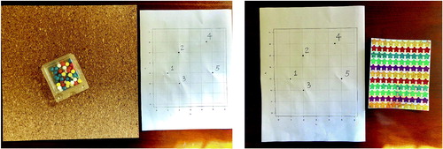
The three-dimensional educational tool kit includes a square bulletin board and pushpins of assorted colors (see the left image of Figure 1). The pushpins are used to display the locations of observations (i.e., points) on a two-dimensional coordinate plane, where the color of each point indicates its membership of a certain cluster. A less expensive alternative, shown in the right image of Figure 1, replaces the bulletin board and pushpins by a piece of paper and a sheet of colorful stickers. In the following discussion, we illustrate a dataset of five observations with two variables, denoted by X₁ and X₂. In particular, the coordinates of the five points are set to be (1, 3), (2, 5), (2, 2), (4.5, 6), and (5, 3). On the bulletin board in Figure 1, we write down a digit from 1 to 5 next to each observation for ease of reference and calculation. Instructors may choose to use a larger number of observations, but please be aware that the expected time to complete the activity increases with the sample size.

Fig. 1 Left: The activity kit that each group of students receive. Right: An alternative activity kit.

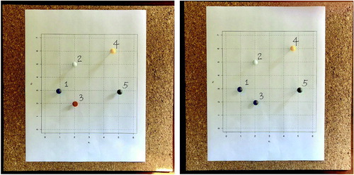
Initially, all pushpins are of different colors, implying that each forms its own singleton cluster. In the process of completing the designed activity, students will change the colors of the pushpins based on the steps of agglomerative hierarchical clustering, reflecting the adjustments of the cluster memberships given a merging criterion. See Figure 2 for a simple demonstration, where the two closest observations (in Euclidean distance) were merged together to form a four-cluster solution. The same procedure also applies to the alternative kit using stickers, that is, students change the colors of certain observations by attaching new stickers on top of the previous ones to complete the process of agglomerative hierarchical clustering in each step. The activity is described in more details in Section 3.2.

Fig. 2 Demonstration of the first step in agglomerative hierarchical clustering, where point 1 and point 3 were merged together.

3.2 Activity Plan

The in-class activity, together with the lesson of the topic on agglomerative hierarchical clustering, can be completed within one lecture of 60–75 min. The class starts with an introduction of clustering analysis and its practical applications. To engage class discussions, instructors may raise some motivating questions, such as:

“Given the set of observations in this plot (shown in a two-dimensional plot with two features), how would you group similar objects into two sets?”

“How would you quantify ‘similarity’ between objects?”

“What is the total number of groups (clusters) needed?”

“Comparing the n-cluster solution and the one-cluster solution, which partition is more homogeneous within each cluster?”

During the interactive conversation with students, the concept of Euclidean distance is reviewed and the method of agglomerative hierarchical clustering is introduced, including the formulations of the three linkage functions as shown in Section 2.

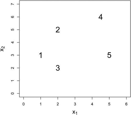
Then, the class is divided into small groups of 3–5 to further investigate agglomerative hierarchical clustering through the designed in-class activity. Each group of students is given activity kit as shown in Figure 1. The five observations presented in Figure 3 were carefully chosen to yield different clustering solutions using each of the single linkage, complete linkage, and group average linkage merging criteria. In addition to the educational tool, each team is also given a worksheet that guides them through the entire activity (please see the supplementary materials for the worksheet and its solution). In the worksheet, students are first given a 5 × 5 distance matrix that represents the pairwise Euclidean distances of the dataset. Alternatively, instructors may provide students with a ruler and let them measure the pairwise Euclidean distances and compute the distance matrix as part of the group activity.$$\text{distance}\mathrm{ }\text{matrix}=\left(\begin{array}{ccccc}0.0& & & & \\ 2.2& 0.0& & & \\ 1.4& 3.0& 0.0& & \\ 4.6& 2.7& 4.7& 0.0& \\ 4.0& 3.6& 3.2& 3.0& 0.0\end{array}\right).$$

Fig. 3 Scatterplot of the dataset.

Following the instructions in the worksheet, each team then realizes agglomerative hierarchical clustering based on each of the three linkage criteria. They are asked to record the cluster solution in each step, starting with “(1), (2), (3), (4), (5)” in Step 0 that represents a five-cluster solution and ending with the single-cluster solution “(1,2,3,4,5)” in Step 4. In Steps 1–3, they need to update the between-cluster distance matrix and identify the smallest, largest, or average distance between clusters given the single linkage, complete linkage, or group average linkage criteria, respectively. Within each team, students are encouraged to take the lead in different roles: for instance, one student may be responsible for taking notes (completing the worksheet questions), and one student may help adjust the colors of the pushpins. All students are expected to participate in the group discussions throughout the activity. The entire activity is expected to be completed within 20 min. In the end, all teams are expected to reach the following results.

• Based on the single linkage criterion:

  Step 0 (5-cluster solution): (1), (2), (3), (4), (5)

  Step 1 (4-cluster solution): (1,3), (2), (4), (5)

  Step 2 (3-cluster solution): (1,2,3), (4), (5)

  Step 3 (2-cluster solution): (1,2,3,4), (5)

  Step 4 (1-cluster solution): (1,2,3,4,5)

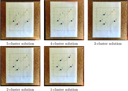
• Based on the complete linkage criterion:

  Step 0 (5-cluster solution): (1), (2), (3), (4), (5)

  Step 1 (4-cluster solution): (1,3), (2), (4), (5)

  Step 2 (3-cluster solution): (1,3), (2,4), (5)

  Step 3 (2-cluster solution): (1,3), (2,4,5)

  Step 4 (1-cluster solution): (1,2,3,4,5)

• Based on the group average linkage criterion:

  Step 0 (5-cluster solution): (1), (2), (3), (4), (5)

  Step 1 (4-cluster solution): (1,3), (2), (4), (5)

  Step 2 (3-cluster solution): (1,2,3), (4), (5)

  Step 3 (2-cluster solution): (1,2,3), (4,5)

  Step 4 (1-cluster solution): (1,2,3,4,5)

Figures 4–6 present the steps of the activity based on the single linkage, complete linkage, and group average linkage criteria, respectively.

Fig. 4 Steps of activity based on the single linkage criterion.

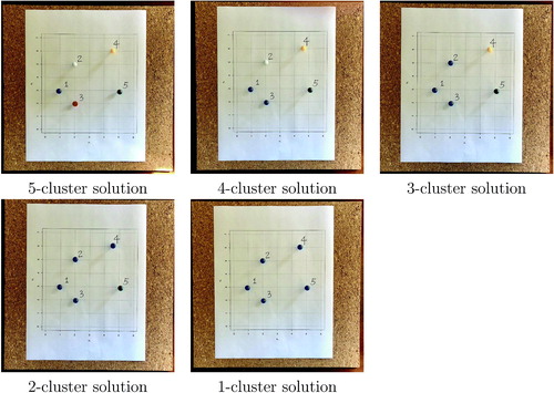
Fig. 5 Steps of activity based on the complete linkage criterion.

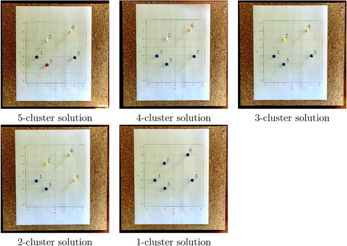
Fig. 6 Steps of activity based on the group average linkage criterion.

After the completion of the group activity, the entire class engages in a follow-up discussion. Instructors may raise leading questions that encourage students to think actively about the reasons behind the same or different solutions based on the three merging criteria. Some possible questions include:

“Why are the 4-cluster solutions the same given different linkage functions?”

“Among the three 2-cluster solutions, which one is the most imbalanced? Why would that happen?”

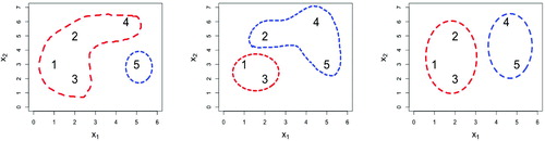
The above questions may lead to the introduction of the chaining and crowding effects. To further clarify these concepts, instructors may present visualization of the chaining and crowding effects using graphs such as those in Figure 7. The left panel displays the two-cluster solution following the single linkage criterion. The relatively large size of the red cluster shows the chaining effect, that is, single observations tend to merge into existing clusters in precedent steps. The middle panel presents the two-cluster solution using the complete linkage criterion. In this case, the Euclidean distances between point 2 and point 1 and between point 2 and point 3 are 2.2 and 3.0, respectively. However, point 2 is grouped with points 4 and 5 together, and the Euclidean distances between point 2 and point 4 is 2.7 and between point 2 and point 5 is 3.6. In other words, point 2 is closer in Euclidean distance to members of the other cluster compared to points of its own group. The right panel is the 2-cluster result based on the group average criterion which seems to offer a compromise solution between the other two approaches and potentially alleviates the chaining and crowding effects.

Fig. 7 Illustration of the 2-cluster solutions based on the single linkage (with the chaining effect), the complete linkage (with the crowding effect), and the group average linkage criteria. The last merging rule offers a compromise solution between the previous two criteria.

If the course is taught at a higher level, other merging criteria such as centroid linkage (Sokal and Mitchener 1958) and mini-max linkage (Bien and Tibshirani 2011) criteria may be introduced. These more recent developments aim to avoid the undesirable chaining and crowding effects that are often associated with the single linkage and complete linkage criteria.

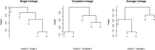
Up till now, students should have a thorough understanding on how clusters are formed using different merging criteria. If time permits, the lesson may continue with software illustration. For instance, instructors could introduce commonly used R functions to realize agglomerative hierarchical clustering, and discuss how to visualize the clustering results by a dendrogram. As an example, instructors may use the following code to demonstrate how use of the hclust() function to analyze the aforementioned five-point dataset.

#Creating the coordinates of the points in the activity x1 <- c(1,2,2,4.5,5) x2 <- c(3,5,2,6,3) data = cbind(x1,x2) # Fit agglomerative hierarchical clustering methods and plot the dendrograms hc.single <- hclust(dist(data), method="single") plot(hc.single) hc.complete <- hclust(dist(data), method="complete") plot(hc.complete) hc.average <- hclust(dist(data), method="average") plot(hc.average)

These R commands will produce the dendrograms as shown in Figure 8.

Fig. 8 The dendrograms produced by R.

Remarks. We have the following observations and suggestions for using the designed activity.

1. When updating the distance matrix between clusters from step to step (see the worksheet in the supplementary materials), instructors may provide assistance to certain groups of students, reminding them of the definition of each merging criterion.

2. It is not obvious to students what the meaning of “height” is in a dendrogram. When presenting the dendrogram (Figure 8) in R, instructors may point out to the class that the “height” at each merging step corresponds to the optimal distance given a linkage criterion. For instance, suppose one follows the complete linkage criterion. At a certain step if cluster s and cluster t are merged together, the merging point that corresponds to the level of “height” in the dendrogram equals to the maximum distance between observations in cluster s and cluster t, namely, $\max \{d_{ij}:X^i\in \mathrm{ }\text{cluster}\mathrm{ }s,X^j\in \mathrm{ }\text{cluster}\mathrm{ }t\}$. Furthermore, such maximum distance (i.e., height) is the smallest among all maximum distances between pairs of clusters obtained in the previous step. In this case, the minimal maximum distance between clusters is the “optimal distance.”

3. According to our teaching experience, one difficulty that some students may have in completing the activity is to determine the maximum distance (minimum distance, or average distance, depending on the linkage criterion) between clusters. At a given step, students need to first carefully identify observations in each cluster and then find out the maximum distance, for example, between each pair of clusters so that they can correctly determine which two clusters are to be merged together in the following step. Another important task in cluster analysis is the selection of the number of clusters. Although there have been a number of available tools in existing literature, choosing the optimal number of clusters is generally regarded as a difficult task. In our real data example, we illustrate the use of elbow method (Thorndike 1953), based on the within-cluster variations to identify the number of clusters to use.

4. The designed class activity also provides instructors with an opportunity to better illustrate chaining and crowding effects with the help of appropriate visualization. We found graphical displays, such as those shown in Figures 7 and 8, helped students grasp the seemingly abstract concepts of chaining and crowding effects more easily.

The aforementioned lesson plan should be sufficient for one regular class period of 60–75 min. After students have a thorough understanding of agglomerative hierarchical clustering, instructors may introduce them a more real dataset where the feature space is of higher dimensions and the number of observations is larger. When working on the real data example, instructors can guide students to make connections to the observations concluded from the simple class activity in the context of the given dataset. For instance, we use a facial recognition dataset in our classes. The data consist of 400 images of 40 different individuals. All of these images were taken between April 1992 and April 1994 at the Olivetti Research Laboratory in Cambridge, UK. Hence, the dataset is also known as the Olivetti Faces dataset. The dataset can be found from the AT&T lab (https://www.cl.cam.ac.uk/research/dtg/attarchive/facedatabase.html). It was also studied in Bien and Tibshirani (2011) in the context of clustering analysis. In this example, the primary goal is to correctly group similar images together. To ease visualization of the clustering results, we recommend working on a subset of available images. In the supplementary materials, readers can find a detailed case study, including sample R commands and the corresponding clustering results, using all of the 10 images from one individual of the Olivetti Faces dataset.

Within the broader curriculum, after other clustering methods are introduced (e.g., k-means clustering, model-based clustering, etc.), instructors may further discuss the comparisons between various clustering methods. In addition, if the topic of classification has been taught, there is a good opportunity to highlight the differences between unsupervised learning and supervised learning when comparing clustering with classification.

4 Summary and Discussion

This article introduces an active-learning class activity. It can be realized by a designed three-dimensional educational tool that is easy to use by statistics instructors. The developed teaching tool is appropriate for a multivariate data analysis course or any course that covers the topic of agglomerative hierarchical clustering. The use of the educational medium encourages students’ in-class participation and active learning, and promotes collaborative teamwork that enhances the understanding of the methodology. The teaching tool can be simplified by plain paper and stickers as a less expensive alternative. In a future project, we are interested in comparing the efficacy and learning outcomes of using different educational tools, including the bulletin board-based three-dimensional tool, the paper-based alternative tool, and the rudimentary method (i.e., the traditional lecture-based lesson).

Supplementary Materials

In the supplementary materials, we include the worksheet and its solution for the activity introduced in Section 3.2. Additionally, a detailed case study that applies agglomerative hierarchical clustering to a subset of the Olivetti Faces datasets is also included with sample R commands and the corresponding clustering results.