Development of an Informal Test for the Fit of a Probability Distribution Model for Teaching

Abstract

Informally testing the fit of a probability distribution model is educationally a desirable precursor to formal methods for senior secondary school students. Limited research on how to teach such an informal approach, lack of statistically sound criteria to enable drawing of conclusions, as well as New Zealand assessment requirements led to this study. Focusing on the Poisson distribution, the criteria used by ten Grade 12 teachers for informally testing the fit of a probability distribution model was investigated using an online task-based interview procedure. It was found that criteria currently used by the teachers were unreliable as they could not correctly assess model fit, in particular, sample size was not taken into account. The teachers then used an interactive goodness of fit simulation-based visual inference tool (GFVIT) developed by the first author to determine if the teachers developed any new understandings about goodness of fit. After using GFVIT teachers reported a deeper understanding of model fit and that the tool had allowed them to take into account sample size when testing the fit of the probability distribution model through the visualization of expected distributional shape variation. Hence, a new informal test for the fit of a probability distribution is proposed.

Keywords:

• Goodness of fit
• Grade 12 teachers
• Informal inference
• Poisson distribution
• Secondary statistics education
• Visual inference tool

1 Introduction

The nature of the statistics taught and assessed in New Zealand secondary schools was significantly impacted by the implementation of the New Zealand curriculum (Ministry of Education 2007). In particular in Grade 12, new simulation-based methods such as bootstrapping and randomization tests were introduced (Pfannkuch et al. 2013) to support students’ statistical inferential reasoning. However, for the requirement that Grade 12 statistics students should compare model probability distributions with experimental distributions, there were no proposed ways on how to teach conceptual understanding of how to assess goodness of fit and on how to informally test the fit of a probability distribution model. The problem was compounded because there was limited research in this area and there did not seem to be a pedagogical method that was statistically sound that would help teachers introduce students to an informal test for goodness of fit.

The purpose of this study was 3-fold. The first purpose was to determine how one could informally test the fit of a probability distribution model and then to develop an interactive goodness of fit simulation based visual inference tool (GFVIT). The second purpose was to find out how some teachers informally test the fit of a probability distribution model, which would inform how an informal test could be currently taught to students. The third purpose was to trial the GFVIT tool on the same teachers for them to reflect on their prior conceptions and to consider the potential benefits for learning how to assess goodness of fit. The trialing of the GFVIT tool with teachers also gave an opportunity to identify any issues with the tool before future research with students. Although the tool can be used for any probability distribution, this paper exemplifies the findings by focusing on the Poisson distribution. Therefore, the research questions regarding some Grade 12 teachers were: (1) What criteria do these teachers use for informally testing the fit of a probability distribution model? (2) What new understandings about goodness of fit emerge when these teachers use the GFVIT tool?

2 Current Teaching Situation in New Zealand

In New Zealand, Grade 12 statistics students undertaking the National Certificate in Educational Achievement (NCEA) can be assessed against seven different statistics achievement standards based on the New Zealand Curriculum (Ministry of Education 2007). Apply probability distributions in solving problems (hereafter referred to as the AppProb Standard) is one of these NCEA statistics Achievement Standards and is externally assessed by the New Zealand Qualifications Authority (NZQA) through a one-hour written exam paper. Students who are assessed against the AppProb Standard are required to investigate situations that involve elements of chance using methods such as calculating and interpreting expected values and standard deviations of discrete random variables, and applying discrete and continuous probability distributions (e.g., uniform, triangular, Poisson, binomial, and normal). Students are required to informally test the fit of the probability distribution model by comparing the model probability distribution with the experimental probability distribution, and concluding that if the model was a “good fit” then the model is a “good model” for the true probability distribution. The method typically used in assessments for informally testing the fit of the probability distribution model is as follows: discuss the assumptions of the model, then compare the features of the model and experimental probability distributions such as mean, variance, and shape, and then use these comparisons to judge the “goodness” of the model as it applies to the true probability distribution.

While the New Zealand Curriculum (Ministry of Education 2007) expects that students learning about probability “acknowledge samples vary,” “compare and describe the variation between theoretical and experimental distributions,” and appreciate “the role of sample size,” there is no guidance provided as to how to teach this objectively. Instead, subjective evaluations are made when comparing theoretical and experimental distributions, using words such as “close” or “similar” and furthermore sample size is not taken into account. Hence, the method proposed for informally testing the fit of the probability distribution model has no clear criteria for making a call about the “goodness of fit.” In contrast, when students are taught about statistical inference they are taught that distributional shape and estimates are affected by the size of the sample and through using bootstrapping and randomization test methods base their conclusions on explicit evidence or criteria. Therefore, it was identified that research was needed to explore how Grade 12 statistics teachers assess the fit of a probability distribution model, as each teacher’s understanding will inform how they teach an informal test to Grade 12 students.

3 Review of Research Literature

Before discussing research involving informally testing the fit of a probability distribution model, informal inferential reasoning research is drawn upon to characterize an informal test for goodness of fit. Such a characterization is needed to theorize how an informal test for goodness of fit could be taught to support the learning of inferential reasoning.

Informal inferential reasoning is defined by Zieffler et al. (2008) as reasoning where students make claims but do not use formal statistical procedures, use available prior foundational conceptual knowledge and articulate evidence for a claim. Firstly, with regard to formal procedures, Dolor and Noll (2015) stated that the rationale for teaching informal approaches to inference is to make formal procedures more accessible. Hence, an informal test for the fit of a probability distribution model should build toward understanding the chi-square goodness-of-fit test, which determines whether the proportions of each outcome of a single categorical variable follow the model probability distribution. Secondly, when considering what prior knowledge students have available within probability modeling learning contexts, many research studies (e.g., Konold and Kazak 2008; Fielding-Wells and Makar 2015) point to students discussing model fit by comparing features of distributions and growing samples. Although these studies do not formally use probability distributions, they do indicate that a learning approach for novices to begin to think about model fit is visually comparing distributions of data, including, thirdly, the ability to use evidence to make a claim. The challenge for making an informal inference, however, is to determine what evidence can teachers draw on that is statistically sound to help students build their conceptual understanding of the goodness-of-fit of a probability distribution model.

Therefore, we define the characteristics of an informal test for the fit of a probability distribution as one that:

• Does not use formal procedures, methods, or language (e.g., test statistic, null hypothesis, chi-square, p-value);

• Draws a conclusion about the goodness of fit of a probability distribution model by looking at, comparing, and reasoning from distributions of data;

• Builds conceptual understanding of the goodness of fit of a probability distribution model; and

• Provides foundations to make the procedures associated with the chi-square goodness of fit test more accessible.

Based on this definition for an informal test for the fit of a probability distribution, only two relevant studies were located: Dolor and Noll (2015) and Roback et al. (2006). In both studies, the teachers involved students in creating and using a set of test samples to assist them to develop initial ideas about what features would and would not support the model distribution being tested. Students were then guided by the teachers to develop their own method for measuring the discrepancy between the model distribution and the sample data using the test samples. Sampling distributions for the student-created test statistics were then generated using simulation and used to provide evidence against the fit of the model for each of the test samples. Dolor and Noll (2015) found that students were able to reason with the simulated sampling distribution created from their own measure of discrepancy, and were able to consider the shape of the sampling distribution in relation to degrees of freedom and to the nature of the measure. In contrast, despite seeing the value in creating their own test statistic, Roback et al. (2006) observed that students did not independently use the simulated sampling distribution to assess whether the test statistic provided evidence against the fit of the model.

A feature of both studies was the generation of the sampling distribution for the measure of discrepancy or test statistic. Although the generation of the sampling distribution would show variation from sample to sample, the variation is for the test statistic, a measure that is not visually connected to the sample distribution and the model probability distribution. Hence, a limitation of this teaching approach is that the test statistic condenses a myriad of understandings into an abstract measure. Another limitation of teaching the use of a single numerical measure as part of a test is that the distributional features of the sample and probability distribution model are devalued; features such as sample space, number of outcomes, variation of individual proportions, influence of sample size, and the interaction between them. For similar reasons, Q-Q (quantile-quantile) plots were not considered in the development of an informal test for the fit of a probability distribution as they require conceptualizing the distributions in terms of quantiles and do not support the visual comparison of sample distribution and the model distribution in terms of distributional shapes. Furthermore, Poisson, binomial, uniform and triangular models are new concepts for Grade 12 students and hence a test that used a visual comparison of features of the model and sample distributions would be more appropriate for teaching.

Simulation-based inference teaching is primarily geared toward the creation and use of a sampling distribution for the test statistic. However, Hofmann et al. (2012) developed a graphical inference method, an inference approach where data plots are used as test statistics. A lineup of plots is generated consisting of the real sample data plot randomly placed somewhere between plots generated from the null hypothesis or a known model. If someone viewing the lineup of plots can identify the real sample data then that gives statistical evidence to support a conclusion that the real sample data does not fit with the null data (the model tested). Such a visual inference method used for teaching fulfills the four characteristics of an informal test defined earlier as it allow students to use an informal procedure, to draw a conclusion about the goodness of fit of a probability distribution model by looking at, comparing, and reasoning from distributions of data, builds conceptual understanding, and provides foundations for the chi-square test. However, a teaching approach using static lineups lacks visual animation and the ability for students to visualize and experience the representative intervals for the expected variation of each proportion in the model, which Dolor and Noll (2015) considered an important idea for students to experience in their study.

Using an example of a jar that contained equal numbers of four different colored beans, they asked students to give representative intervals for how many beans of each color they would expect to observe in samples of 100, for example, 22–28 for each color. Students were specifically told to consider the expected variability from sample to sample when creating these representative intervals. Dolor and Noll included this task in their learning trajectory to generate discussion around unusualness and to encourage thinking around how to judge sample distributions as being similar or different to the model distribution. However, Dolor and Noll observed that students found it challenging to create the representative intervals, as they had not built up enough experience working with repeated samples.

Teachers building up student experience of working with repeated samples for informal statistical inference is a feature of the work of Wild et al. (2011) as their animations visually track sample to sample variation in summary statistics such as medians or in the case of bar graphs the variation in each proportion. For example, the sample to sample variation in medians of boxplots or variation in proportions of bar graphs are tracked and shown interactively building up into intervals overlaid onto the display plot, allowing students to visualize the noise or variation around the signal. The question is whether a reliable method, based on students experiencing and visualizing the noise around a distributional shape signal, can be determined for an informal goodness-of-fit test for a probability distribution model.

Sketching distributional shape has a limited research base. From the work of Arnold (2013) on Grade 9 students, where the research was focused on sample-to-population inference, it was identified that students intuitively tended to overfit distributions by following the outline of dot plots. Hence, Arnold (2013) encouraged students to focus on sketching the signal in distributional shape using smooth representative curves. In her research she used large sample dot plots and a context where students could draw on their personal contextual knowledge to inform their sketch. However, using context in determining the appropriateness of a model can be problematic as Casey and Wasserman (2015) found that the teachers in their study ignored points when fitting a line of best fit to bivariate sample data because they used contextual knowledge about the population relationship. It is also questionable whether contextual knowledge should be part of any criteria for an informal test of goodness of fit. On the other hand, when engaging with probability distributional modeling students can work with data simulated from the probability distribution alongside real data observations and do not need to draw on contextual knowledge. Indeed, in the research of Fielding-Wells and Makar (2015), when young students played a game of addition bingo, the probability distribution model of which is triangular, they produced over-fitted shape sketches of their results. These shape sketches of the students’ sample distributions were then laid on top of each other. Although individually the over-fitted shape sketches did not show the shape of the distribution, collectively they started to paint a picture of a triangular mountain. This approach not only reinforces ideas about signal and noise but also why a good model is unlikely to be an over-fitted shape.

Another consideration is sample size and how to take it into account when making informal inferences. To learn about how the shape of small samples may not look like the model and the effect of sample size on shape, Konold and Kazak (2008) asked middle-school students to generate simulations using varied sample sizes from a discrete triangular distribution and to rate the degree of fit of the expected distribution either as “bad,” “OK,” or “great.” Furthermore, Konold and Kazak and others (e.g., Lehrer, Jones, and Kim 2014; Kazak, Pratt, and Gökce 2018) have used simulation to explore the relationship between the shape of the model distribution and the shape of data simulated from the model and encouraged students to use shape as one of their criterion for assessing model fit. Hence, from a review of the literature it would seem that within a software driven modeling environment that over-fitted distributional shapes could be tracked from simulated sample to simulated sample from the model and could be used to develop a new informal test for teaching the fit of a probability distribution model.

With regard to the software interface for teaching simulation-based modeling, there are two important considerations: student confusion between real data and simulated data (Gould et al. 2010; Pfannkuch, Wild, and Regan 2014) and whether the inference is about the true, unknown population/probability distribution or the known probability model distribution (Konold et al. 2011; Pfannkuch and Ziedins 2014). In the latter case there are examples of probability modeling, such as drawing objects from a bag at random, where the probability model is unknown to the students (Fielding-Wells and Makar 2015) and hence from the student perspective, their inference is about the true and unknown probability distribution, not directly about the model probability distribution. In these situations the model is the same as the truth but in other situations the model may not be the truth, only an approximation to the truth. Hence, in these other situations the data collected from the real situation can only be used to infer the true probability distribution and not the model probability distribution, as the data are not generated from the model. To prevent these confusions Fergusson (2017) proposed a statistical modeling framework (Figure 1) that clearly separates the real world and the model world. The framework allows for the separation but connection of data that are observed in the real world and data that are generated from a model, and the separation but connection of the true unknown random process that is being modeled and the model itself.

Fig. 1 Statistical modeling framework (Fergusson 2017, p. 62).

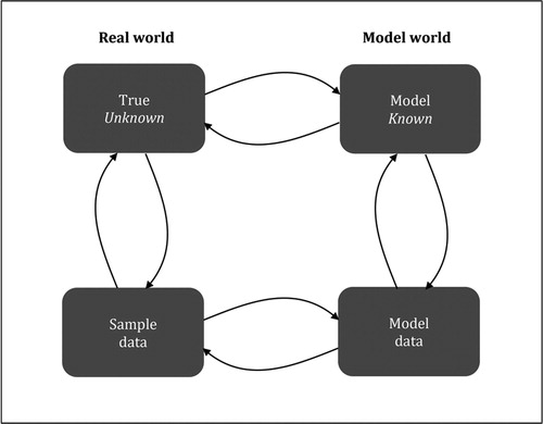
Within this framework, the arrows that connect each of the four components are bi-directional and represent the shuttling between knowledge from both components during a statistical modeling activity (c.f. Wild and Pfannkuch 1999). For example, the connection between the true distribution or process to sample data represents the consideration of how the data were generated (e.g., through the use of random sampling from a population). The connection from sample data to the true distribution or process is inferential in nature, and represents the use of the sample data to obtain estimates for features of the true distribution or process.

4 Method

A small exploratory study was conducted where the priority of the research was to collect rich information, not to obtain a representative sample or to generalize the findings to a wider population (Creswell 2015). A mixed methods research design was used as the research questions could be better answered using a combination of quantitative and qualitative methods. Structured task-based online self-interviews, where participants are asked to complete a task and verbalize in writing their reasoning and thoughts, were used. This method is similar to that used by Casey and Wasserman (2015), who were measuring teachers’ understanding of informal lines of best fit. Specifically, for Task One reported in this article, a quantitative method, a randomized experiment, was embedded within a qualitative data collection method.

Data were collected from participants over a four-week period through a task-based self-interview conducted in an online environment, which allowed participation of teachers from a range of locations in New Zealand. The online environment gave participants the flexibility of completing each task at separate times. The tasks, including some parts of tasks, were presented one at a time and once answered could not be revisited.

4.1 Participants

The participants in the overall study were 17 Grade 12 statistics teachers from a range of New Zealand high schools who had taught the Grade 12 probability distribution standard. Recruitment of teachers was through an advertisement placed on the NZ statistics teachers Facebook page. In total, 28 teachers responded with 17 completing at least the first out of five tasks. However, for the two tasks reported in this paper, ten and nine teachers completed them, respectively. Of the ten, four had completed an undergraduate degree with a major in statistics or equivalent.

4.2 Tasks

4.2.1 Task One

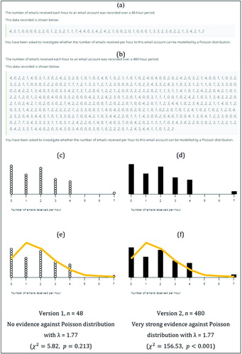
Task One involved teachers investigating whether the number of E-mails received per hour to an E-mail account could be modeled by a Poisson distribution. Task One was a randomized experiment and thus there were two versions of this task: Version 1 had a small dataset (n = 48, see Figures 2(a) and (c)) and Version 2 a large dataset (n = 480, see Figures 2(b) and (d)). In both versions all questions were identical and the sample distributions used were identical in terms of outcomes and proportions (see Figures 2(c) and (d)). Teachers were randomly allocated to one of the two versions. The first part of the task asked teachers to describe the steps they would take to complete the investigation, which is not reported in this article. The second part required teachers to sketch the shape of the sample distribution and then they were shown the sample data with the theoretical model, the Poisson distribution, overlaid and asked to discuss the appropriateness of the Poisson model in terms of the visual fit of the model to the sample data. For Version 1, the chi-square test gave no evidence against the Poisson distribution being a good fit for the sample distribution whereas Version 2 gave very strong evidence against the Poisson distribution. Task One was designed to test the conjecture that teachers do not take sample size into account when assessing the fit of a probability distribution model to sample data and to explore what criteria and reasoning teachers use to informally assess the goodness of fit.

Fig. 2 Key design features of Task One.

4.2.2 Task Two

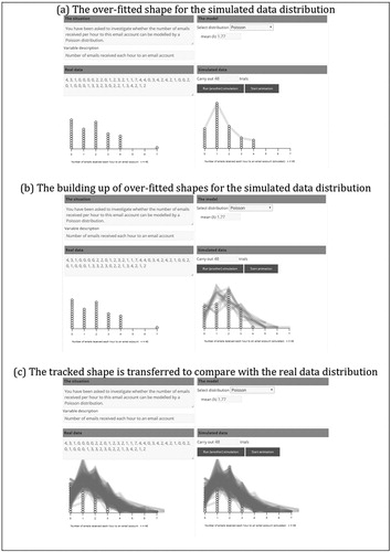
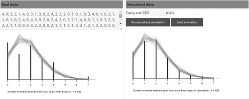
Task Two involved a simulation-based modeling tool (http://learning.statistics-is-awesome.org/modeling-tool/) designed by the first author, the researcher for the study. The tool was designed to address potential issues identified in the literature review, namely: sample data collected from the real situation being confused with simulated data generated from the model; and sample size not being taken into account when informally testing probability distribution models. Two noteworthy features of the tool are: (1) the left-hand side of the screen displays information related to the real situation being modeled and the right-hand side of the screen displays information related to the model being used (see Figure 1); and (2) the tracking of the over-fitted shape for the simulated data from the model. This allows the learner to visualize and experience the expected variation in shape using animation that simulates samples the same size as the real data and to transfer that visualization to the sample distribution to informally test the fit of a probability distribution model. Figure 3 shows screen shots of the three key stages of using the tool to informally test the fit of a probability distribution model.

Fig. 3 Screenshots demonstrating the use of the interactive tool to informally test the fit of a probability distribution model for Task Two.

For Task Two teachers were first guided how to use the tool using two contrasting examples. They were then given the sample data they were presented with in Task One to use the tool to assess the fit of the Poisson model. Teachers were then asked what understandings about informally fitting a probability distribution model, if any, the tool helped to clarify for them and the benefits the tool might have for building students’ understanding of model fit.

5 Analysis of Data

Because Task One was a randomized experiment, significance tests were conducted to determine whether there was a difference between the responses of the two groups of teachers. Qualitative data for Task One were analyzed using a thematic approach. The goal of a thematic analysis (Braun and Clarke 2006) is to identify patterns of meaning across a dataset using six phases: (1) familiarize oneself with data, (2) generate initial codes, (3) search for themes, (4) review themes, (5) define and name themes, and (6) produce a report. For Task Two a summary of teacher reflections is presented.

5.1 Task One Results

The results for Task One are divided into three parts. The first part considers the effect of the sample size: Version 1 (participants shown a sample of size 48), Version 2 (participants shown a sample of size 480). The second part determines the criteria the teachers used for sketching shapes of distributions, while the third part determines the criteria the teachers used for assessing the visual fit of the model.

5.1.1 Randomized Experiment

Five teachers were randomly allocated to Version 1 and five to Version 2 of Task One. It was conjectured that there would be no overall difference between the two groups of teachers when analyzing the responses to questions within the task.

5.1.2 Criteria Described for Sketching Shapes of Distributions

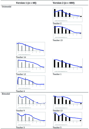
The shape sketches drawn by the teachers for each version of the task were similar, despite the sample sizes being quite different (Figure 4). Of note is that two teachers for both versions sketched a bimodal distributional shape. In the case of Version 2 (n = 480), the bimodality visible in in the distribution should be interpreted as a very strong signal for the distribution as the outcomes associated with outcomes 0 and 2 would be over 100 each for a total sample size of 480.

Fig. 4 Shape sketches for Task One matched by pairs of visually similar sketches across Versions 1 and 2 of the task.

After the teachers sketched the distribution they were asked to describe the criteria they used to sketch the shape, to which nine of the ten teachers responded. The criteria they used were categorized and are presented in Table 1. Each teacher was placed in only one category. Interestingly 7 of the 9 descriptions used knowledge beyond what could be seen in the distribution. The outline criterion involved the fitting and inferring of a smooth shape, whereas the use of the context criterion involved drawing on teachers’ presumptions about the behavior of E-mails to the E-mail account. The leveling criterion involved using knowledge about how much variation there would be between different samples, while the model criterion involved using knowledge about the proposed model for the number of E-mails arriving per hour. None of the teachers made reference to how much data was represented or the sample size and all of the teachers drew sketches that were based on all outcomes in the distribution.

Table 1 Categories of criteria described to sketch the shape of a distribution.

Criterion	Description	Example excerpt	Number of teachers
Outline	The sketch should be a smooth outline of the data distribution, with the peak(s) or highest point(s) determined by the outcome(s) with highest frequency.	“Imagining how a heavy blanket would drape itself over the columns” [Teacher 13]	3 [Teachers 5, 12, 13]
Context	The sketch should be informed by contextual knowledge of the variable. Use context to decide which features of data distribution to incorporate in shape.	“It will be bimodal because there are a lot of hours in the middle of the night when no-one sends me an email” [Teacher 3]	3 [Teachers 1, 3, 9]
Leveling	The sketch should try to balance out the heights of each bar or stack of dots to take into account sampling variability or noise.	“I thought that the up and down at 1 to 4 was due to sampling variability, so I didn’t follow that exactly” [Teacher 4]	2 [Teachers 4, 16]
Model	The sketch should be based on the model distribution. Use model to decide which features of data distribution to incorporate in shape.	“Assumed a Poisson with mean around 1 or 2” [Teacher 2]	1 [Teacher 2]

5.1.3 Informally Testing the Fit of a Probability Distribution Model

Teachers were asked to discuss the appropriateness of the Poisson model in terms of the visual fit of the model to the sample data, to which all ten teachers responded. The expected good responses are illustrated in Figure 5.

Fig. 5 Examples of good responses to the two versions of Task One for assessing the fit of the Poisson distribution to the sample data.

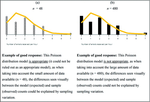
Despite the fact that the two versions of the task had been designed to elicit different responses, three Version 1 teachers (4, 9, 12) responded the same way as three Version 2 teachers (5, 13, 15) by discussing the Poisson distribution model as being appropriate. Only three teachers (4, 9, 13) made reference to the sample size when considering the fit of the proposed model: two Version 1 teachers (4, 9) and one Version 2 Teacher (13). However, three of the six teachers, who concluded the proposed model was appropriate, expressed a lack of confidence in their conclusion, such as Teacher 13 who stated “things that make me less confident are …” Therefore, in addition to sample size not being considered by most of the teachers when informally testing the fit of a probability distribution, the reluctance to commit to a conclusion about the appropriateness of the model suggests there are issues with the criteria used by the teachers.

Consequently, six criteria that were used by teachers to decide on the visual fit of a model were identified (Table 2). Nine of the ten teachers used more than one criterion. The two most used criteria to compare the proposed model with the sample data—individual outcomes and shape—were used by teachers irrespective of the version of the task they completed. These two criteria are related as the shape of the model and sample distribution are based on individual outcomes within each distribution. However, teachers did not seem to recognize the connection between individual outcomes and shape in their descriptions. For example, Teacher 4 explained that she was “concerned about the high frequency of zero and the low frequency of one,” making use of the individual outcomes criterion, and then went on to explain, “but apart from those, the shape of the graph is what I would expect from a sample of 48,” making use of the shape criterion. She qualified this further using the sampling variation criterion, stating that “the high frequency of zero and the low frequency of one are within what might be expected due to random variation in a sample from a Poisson distribution.” This teacher appeared to disconnect the shape of the sample from each outcome within the distribution and its associated frequency, by suggesting the shape of the distribution could be described without using two of the outcomes. Two teachers (3, 4) went beyond a data-fitting exercise and discussed whether the proposed model would be useful and whether the conditions of the model were met. As all of the criteria identified in Table 2 involve a comparison between what was expected and what was observed, sample size should be taken into account. For example, the measures criterion was typically used to compare the mode of the sample distribution and the mode of the proposed model. The same three teachers who discussed sample size when assessing the visual fit of the Poisson distribution to the sample data also used the sampling variation criterion (4, 9, 13).

Table 2 Categories of criteria teachers used to assess the visual fit of the model.

Criterion	Description	Example excerpt	Number of teachers
Individual outcomes	The observed counts for each outcome in the sample data are similar/different to the expected counts for each outcome under the model.	“The model underestimates the number of hours where no emails are received (and somewhat for the number of hours where 4 emails have been received), and overestimates the number of hours where 1 email is received” [Teacher 1]	8 [Teachers 1, 2, 3, 4, 5, 9, 13, 16]
Shape	The shape of the sample distribution is similar/different to the shape of the model distribution.	“This distribution is similar to the Poisson distribution in that: it is skewed to the right“ [Teacher 13]	7 [Teachers 4, 5, 9, 12, 13, 15, 16]
Measures	Measures like the mean, median, mode, range and standard deviation are similar/different for the sample and model distributions.	“The mode of the Poisson distribution is 1, the mode for the emails is 0” [Teacher 9]	4 [Teachers 5, 9, 13, 16]
Sampling variation	The differences between observed counts and the expected counts can (not) be explained by sampling variation, including sample size.	“The high frequency of zero and the low frequency of one are within what might be expected due to random variation in a sample from a Poisson distribution” [Teacher 4]	3 [Teachers 4, 9, 13]
Combined outcomes	The observed counts across a subset of outcomes in the sample data are similar/different to the expected counts across a subset of outcomes under the model.	“The fitted model has the number of emails received, 0, 1 and 2, as the most common which does fit that ‘skewed to the lower end’ aspect of a Poisson dist. as well” [Teacher 12]	2 [Teachers 2, 12]
Alternative	The proposed model is (not) a better fit than an alternative model	“A normal dist. bell shaded curve does not appear to match” [Teacher 12]	1 [Teacher 12]

5.2 Summary of Findings for Task One

Teachers used a variety of criteria to sketch the shape of a distribution, and these criteria show that sample size is not taken into account and that other factors not seen in the data distribution are also used when shape sketching. Teachers also used a variety of criteria to assess the fit of a probability distribution model, most commonly comparisons of shape and of expected counts versus observed counts. However, these criteria appear unreliable as they did not allow teachers to correctly assess the fit of a probability distribution model.

5.3 Task Two Results

For Task Two, teachers were guided through the use of the new simulation-based tool for probability distribution modeling and then asked to reflect on what they had learned. Nine of the ten teachers completed this task. These reflections highlighted three potential benefits of using the tool: to reinforce a modeling perspective, to develop specific understandings for probability distributions, and to informally test the fit of a probability distribution model.

5.3.1 Using the Tool to Reinforce a Modeling Perspective

Teachers commented on how using the tool helped support the separation and connection between the real world and the modeling world, making statements such as:

I really like how you can compare your experimental data to the modeled data side by side [Teacher 5]

The connection between the visuals (real life, simulated data from a theoretical distribution) are very clear. … Being able to take the tracked shape and transfer it over to the real life data makes it easy to see the similarities and differences, as well as understanding where the tracked shape came from [Teacher 1]

Teachers were also positive about how the tool kept the focus on probability distributions as models and reinforced the notion that models were an approximation of reality:

Allows students to explore several different models easily [Teacher 3]

The fitted model isn’t necessarily a perfect fit to the real data which is something students can struggle with [Teacher 12]

The possibility of more than one probability distribution fitting the data can be seen [Teacher 9]

The inexact nature of fitting a model [Teacher 3]

The design of the tool in terms of layout and interface was also seen by teachers as intuitive and the use of visualization was perceived as being beneficial to student learning and engagement:

It will be useful for students to simulate samples from a variety of distributions quickly … Seeing sampling variability with the shadowing allowing them to hold multiple iterations of a simulation in their head at once [Teacher 4]

I have found that with other visualization tools (e.g., the ones from iNZight) these help to engage students [Teacher 12]

5.3.2 Using the Tool to Develop Specific Understandings for Probability Distributions

Teachers were positive about how the tool could allow students to learn more about the features of different probability distributions through seeing the data generated from the models.

The comments made by teachers regarding specific understandings for probability distributions that use of this tool could support were in summary:

• Visualization of different probability distributions

• Impact of change of parameter(s) on the shape of the probability distribution

• Visualization of randomness (variation within the distribution) through use of simulations

• Expectations for amount of distributional shape variation and the effect of sample size.

5.3.3 Using the Tool to Informally Test the Fit of a Probability Distribution Model

Across the responses, teachers were in agreement that the tool could allow students to make more secure conclusions regarding the fit of a probability distribution model to sample data. This potential benefit was demonstrated by the responses given by Teacher 13. Presented with Version 2 of Task Two (see Figure 6), this teacher had initially described that the proposed Poisson model was a reasonable fit to the sample data.

Fig. 6 Version 2 of Task Two, which shows the sample distribution (n = 480) with the model probability distribution overlaid on the same graph.

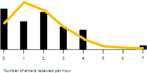
The Poisson model gives a reasonable approximation for the true distribution of emails [Teacher 13]

However, after using the simulation-based modeling tool in Task Two (see Figure 7), this teacher was able to incorporate and visualize the variation associated with a sample distribution of size 480 when considering the fit of the model, as shown in the following excerpt:

Fig. 7 An example of how the new simulation-based modeling tool could have been used by Teacher 13 to test the fit of the probability distribution model.

Gives me a much, much better idea about the amount of expected variation between the experimental data and the model—much less than I expected! [Teacher 13]

Teacher 13 was not alone in reflecting on how the tool had helped enhance her personal understanding of probability distribution modeling, as seen in the excerpts that follow:

It has also really clarified for me that your data doesn’t have to fit the model exactly, as each simulation of the model will give slightly different results. As long as your data is within the range of values from running the simulation, then it is ok. [Teacher 5]

The amount of data collected impacts on the accuracy of the model selection. This is not something I recall explicitly teaching to date, and now I will. [Teacher 9]

5.4 Summary of Findings for Task Two

Teachers were positive about potential benefits of the new simulation-based modeling tool, and identified ways that the tool could reinforce a modeling perspective and support development of understanding for features of probability distributions. Teachers also communicated that the tool had allowed them to take into account sample size when testing the fit of the probability distribution model through the visualization of expected distributional shape variation.

6 Discussion

The purpose of this study was to explore how teachers informally test the fit of a probability distribution. The research questions regarding some Grade 12 teachers, which are now addressed, were: (1) What criteria do these teachers use for informally testing the fit of a probability distribution model? (2) What new understandings about goodness of fit emerge when these teachers use the GFVIT tool?

6.1 Informally Testing the Fit of a Probability Distribution Model

Teachers used a variety of criteria to informally test the fit of a probability distribution model, most commonly comparisons of shape and of expected counts versus observed counts. The comparison of model counts (expected counts) and sample counts for outcomes (observed counts) as a criterion is similar to findings from Lehrer, Jones, and Kim (2014), who found that students compared model statistics with sample statistics as their criterion for model fit. However, comparisons of expected counts and observed counts need to take into account sample size. Additionally, to use sample size as part of an informal test for the fit of a probability distribution model, teachers need knowledge of expected variation of either the model proportions or the sample proportions. It appears in this research that teachers had difficulty visualizing this variation, similar to how the students in Dolor and Noll’s (2015) study lacked experience with expected variation for group proportions. It should be noted that there was high level of alignment between the criteria used by teachers for informally testing the fit of a probability distribution model and the criteria typically used by NZQA assessments. Even though a guideline was found in one government produced resource regarding sample size that samples of at least 200 should show a shape similar to the underlying probability distribution, three out of five teachers made the incorrect call about the fit of the probability distribution model for Version 2 of Task Two, which had a sample size of 480.

The limitation of comparing the probability distribution model counts (expected counts) with the sample data counts (observed counts) extends to the comparison of distributional shapes. The use of shape as a criterion for probability model testing appears to be problematic. First, the concept of distributional shape is not useful for probability distribution models with nominal categorical variables and also for probability distribution models that are shaped irregularly. Second, from a probability modeling perspective, the use of “shape” becomes a probabilistic interpretation of what outcomes are possible (using sample space) and which are more likely to happen or not (using proportions). The inconsistency of the distributional shape sketches for small sample sizes demonstrated by teachers in the study perhaps indicates that a probabilistic interpretation of shape is challenging.

6.2 Emergent Understandings When Using the Tool

Teachers made positive comments about the new simulation-based modeling tool and reflections made suggest that use of the tool could allow for a more reliable informal test of the fit of a probability distribution model. Teachers also communicated that the tool had allowed them to take into account sample size when testing the fit of the probability distribution model through the visualization of expected distributional shape variation and that the layout of the tool supported the connections between the real world and model world. However, no mention was made that the tool helped to distinguish what was being estimated, the true unknown population or the known probability distribution model. The new informal test of the fit of a probability distribution model displayed all of the characteristics that we defined for such a test.

6.3 Limitations of Research

As this study involved a small self-selected sample of 17 teachers, the results cannot be generalized to all teachers. However, the results can be used to indicate potential issues and suggest areas that could need further research regarding teaching model testing. It should be noted that four of the ten teachers who completed all tasks had statistics majors or equivalent, which is higher than would be typically found among Grade 12 Statistics teachers. The data were collected for this study using an online structured self-interview and the researcher was unable to follow up unclear responses with teachers. Tasks were completed by each teacher in a range of environments. There is no way for the researcher to determine if they were completed independently, and so other unknown factors may contribute to what was described in responses. There may be other ways to test the fit of a probability distribution model without overlaying the model line on the data. Therefore, this research only shows one specific method that could be used. Although a randomized experiment was used to test the effect of sample size on teachers’ conclusion for the visual fit of the probability distribution model, the group sizes were small (five each), and therefore any conclusions are tentative.

6.4 Recommendations for Future Research

This research included the development, for teaching, of a new informal test for the fit of a probability distribution model and a simulation-based modeling tool, GFVIT, needed to perform this test. The theoretical basis of this new informal test for the fit of a probability distribution model needs further research. As this was an exploratory study, the trialing of GFVIT with the teachers could only indicate its viability for student learning. Follow up studies are now needed to investigate whether Grade 12 students can understand and interpret this new informal test for the fit of a probability distribution model using GFVIT. Further research is also needed regarding how to teach probability distribution modeling using the new test and whether use of the new test improves teacher as well as student understanding of probability distribution modeling. The new informal test for the fit of a probability distribution model is also an informal test for significance. Care needs to be taken when interpreting the test output, particularly as students can incorrectly interpret large p-values as evidence the null hypothesis (the probability distribution being modeled) is true (e.g., Reaburn 2014). The new simulation-based modeling tool allows a teaching approach where students can quickly change the parameters of a probability distribution model, and track over-fitted shapes for the simulated distributions to show more than one probability distribution could “fit” the sample data. Research could investigate whether teaching that multiple models could “fit” the sample data helps students understand why they cannot accept the null hypothesis.

7 Conclusion

This study was initiated following the identification of a problem with the current method for teaching an informal test for the fit of a probability distribution model, as assessed by the AppProb Standard. The main issues with the current method are the difficulty of taking into account (1) sample size and (2) the expected variation of sample proportions when comparing model proportions with sample proportions, without visual representations of the expected variation or without using a test for significance that uses a numerical test statistic and associated procedures. Research suggested students struggle to separate the real world from the model world in their thinking about probability distribution modeling. To resolve the issue with the current method for informally testing the fit of a probability distribution model, the statistical modeling framework (Figure 1) was used as the basis for the design of a new simulation-based modeling tool that allows the teaching of graphical inference, resulting in a new informal test for the fit of a probability distribution model. The new informal test is the first time that one has been proposed and therefore makes a sound contribution to teaching and research.

ORCID

Anna Fergusson http://orcid.org/0000-0002-1987-8150

Maxine Pfannkuch http://orcid.org/0000-0002-2202-9678

References

- Arnold, P. (2013), “Statistical Investigative Questions. An Enquiry Into Posing and Answering Investigative Questions From Existing Data,” Doctoral thesis, University of Auckland, New Zealand, ResearchSpace@Auckland, available at http://hdl.handle.net/2292/21305
- Braun, V., and Clarke, V. (2006), “Using Thematic Analysis in Psychology,” Qualitative Research in Psychology, 3, 77–101. DOI: 10.1191/1478088706qp063oa.
- Casey, S. A., and Wasserman, N. H. (2015), “Teachers’ Knowledge About Informal Line of Best Fit,” Statistics Education Research Journal, 14, 8–35.
- Creswell, J. W. (2015), A Concise Introduction to Mixed Methods Research, Thousand Oaks, CA: SAGE.
- Dolor, J., and Noll, J. (2015), “Using Guided Reinvention to Develop Teachers’ Understanding of Hypothesis Testing Concepts,” Statistics Education Research Journal, 14, 60–89.
- Fergusson, A.-M. (2017), “Informally Testing the Fit of a Probability Distribution Model,” Masters dissertation, University of Auckland, New Zealand, ResearchSpace@Auckland, available at http://hdl.handle.net/2292/36909.
- Fielding-Wells, J., and Makar, K. (2015), “Inferring to a Model: Using Inquiry-Based Argumentation to Challenge Young Children’s Expectations of Equally Likely Outcomes,” in Reasoning About Uncertainty: Learning and Teaching Informal Inferential Reasoning, eds. A. Zieffler and E. Fry, Minneapolis, MN: Catalyst Press, pp. 1–28.
- Gould, R., Davis, G., Patel, R., and Esfandiari, M. (2010), “Enhancing Conceptual Understanding With Data Driven Labs,” in Data and Context in Statistics Education: Towards an Evidence-Based Society. Proceedings of the Eighth International Conference on Teaching Statistics, Ljubljana, Slovenia, eds. C. Reading, Voorburg, The Netherlands: International Statistical Institute.
- Hofmann, H., Follett, L., Majumder, M., and Cook, D. (2012), “Graphical Tests for Power Comparison of Competing Designs,” IEEE Transactions on Visualization and Computer Graphics, 18, 2441–2448. DOI: 10.1109/TVCG.2012.230.
- Kazak, S., Pratt, D., and Gökce, R. (2018), “Sixth Grade Students’ Emerging Practices of Data Modelling,” ZDM, 50, 1151–1163. DOI: 10.1007/s11858-018-0988-3.
- Konold, C., and Kazak, S. (2008), “Reconnecting Data and Chance,” Technology Innovations in Statistics Education, 2.
- Konold, C., Madden, S., Pollatsek, A., Pfannkuch, M., Wild, C., Ziedins, I., Finzer, W., Horton, N., and Kazak, S. (2011), “Conceptual Challenges in Coordinating Theoretical and Data-Centered Estimates of Probability,” Mathematical Thinking and Learning, 13, 68–86. DOI: 10.1080/10986065.2011.538299.
- Lehrer, R., Jones, R., and Kim, M. (2014), “Model-Based Informal Inference,” in Sustainability in Statistics Education. Proceedings of the Ninth International Conference on Teaching Statistics (ICOTS9, July, 2014), Flagstaff, Arizona, USA, eds. K. Makar, B. de Sousa, and R. Gould, Voorburg, The Netherlands: International Statistical Institute.
- Ministry of Education (2007). The New Zealand Curriculum, Wellington, New Zealand: Learning Media Limited.
- Pfannkuch, M., Forbes, S., Harraway, J., Budgett, S., and Wild, C. (2013), “Bootstrapping Students’ Understanding of Statistical Inference,” Summary Research Report for the Teaching and Learning Research Initiative, available at http://www.tlri.org.nz/sites/default/files/projects/9295_summary/%20report.pdf.
- Pfannkuch, M., Wild, C. J., and Regan, M. (2014), “Students’ Difficulties in Practicing Computer-Supported Statistical Inference: Some Hypothetical Generalizations From a Study,” in Mit Werkzeugen Mathematik Und Stochastik Lernen [Using Tools for Learning Mathematics and Statistics], eds. T. Wassong, D. Frischemeier, P. Fischer, R. Hochmuth, and P. Bender, Wiesbaden, Germany: Springer Spektrum, pp. 393–403.
- Pfannkuch, M., and Ziedins, I. (2014), “A Modeling Perspective on Probability,” in Probabilistic Thinking: Presenting Plural Perspectives, eds. E. Chernoff and B. Sriraman, New York, NY: Springer, pp. 101–116.
- Reaburn, R. (2014), “Introductory Statistics Course Tertiary Students’ Understanding of p-Values,” Statistics Education Research Journal, 13, 53–65.
- Roback, P., Chance, B., Legler, J., and Moore, T. (2006), “Applying Japanese Lesson Study Principles to an Upper-Level Undergraduate Statistics Course,” Journal of Statistics Education, 14. DOI: 10.1080/10691898.2006.11910580.
- Wild, C. J., and Pfannkuch, M. (1999), “Statistical Thinking in Empirical Enquiry,” International Statistical Review, 67, 223–248. DOI: 10.1111/j.1751-5823.1999.tb00442.x.
- Wild, C. J., Pfannkuch, M., Regan, M., and Horton, N. J. (2011), “Towards More Accessible Conceptions of Statistical Inference,” Journal of the Royal Statistical Society, Series A, 174, 247–295. DOI: 10.1111/j.1467-985X.2010.00678.x.
- Zieffler, A., Garfield, J., delMas, R., and Reading, C. (2008), “A Framework to Support Research on Informal Inferential Reasoning,” Statistics Education Research Journal, 7, 40–58.