Teaching the Complexity of Dependence With the Triplet Game

Abstract

Students often struggle with the concept of dependence of events or random variables. We present a simple coin flipping game that yields surprising results due to the dependencies within the game. The game is simple enough for young children to understand and play, yet complex enough to yield results that are counterintuitive to even most graduate students. We discuss how to implement the game in a classroom, suggest two problems from the game for students to solve, and present several solutions to the problems.

KEYWORDS:

• Coin flipping
• expected value
• randomness
• simulation

1 Introduction

Students new to the study of probability and statistics face the challenge of understanding the concept of dependence between events or random variables. The most common error is to assume independence, which usually simplifies calculations, but often leads to error. William Kruskal, former president of the American Statistical Association, chided that kind of error, calling it mathematical laziness: “… one may well ask why the assumption of independence is so widespread. One answer is ignorance. … Far more important than simple ignorance, in my opinion, is seductive simplicity. It is so easy to multiply marginal probabilities, formulas simplify, and manipulation is relatively smooth, so the investigator neglects dependence, or hopes that it makes little difference. Sometimes the hope is realized, but more often dependence can make a tremendous difference” (Kruskal 1988, p. 933). As educators, we owe it to our students to remove their ignorance and share the dangers of simplicity.

One approach to teaching dependence uses games of chance. We do so with a coin flipping game, one that is simple enough for elementary school students to learn and play, yet one that yields results that very few graduate students foresee. This article describes the game and discusse its application in the classroom. We provide multiple solutions to problems raised in the game. These solutions include both Monte Carlo simulations in Excel and R, as well as motivations for closed form solutions. The mathematical background necessary to understand the solutions vary, which allows sharing this game with a wide range of students. We also provide intuition to help students better understand the counter-intuitive results.

The Guidelines for Assessment and Instruction in Statistics Education (GAISE) College Report (2016) suggests two areas of emphasis in the teaching of statistics: (1) teach statistics as an investigative process of problem-solving and decision-making and (2) give students experience with multivariable thinking. We suggest that our coin-flipping game embraces both recommendations. We are not, of course, the first to consider coin flipping to teach probability. Several authors (Morgan and Morgan 1984; Popham and Sirotnik 1992; Maxwell 1994) have coin flipping exercises to introduce and explain p-values. Others use coin flipping to explain probability to students as young as middle school (Braun et al. 2014; Degner 2015). We are also not the first to use Monte Carlo simulation to estimate the solutions of difficult problems (Hodgson and Burke 2000; Vaughan and Berry 2005; Sigal and Chalmers 2016). Jamie (2002) provided an excellent review of the computer simulation literature and discussed its impact on students. Most recently, Miller and Sanjurjo (2018) found that even established researchers err when calculating conditional expectations in sequential data. Their investigation into the hot hand fallacy discovered a bias in how many researchers measure conditional dependence of outcomes in sequential data.

2 The Triplets Game

Triplets is a game that consists of two players observing a sequence of flipped coins. Each player selects one of the eight possible triplets of outcomes when flipping a fair coin three times (TTT, TTH, THT, HTT, THH, HTH, HHT, HHH). They may not select the same triplet. One of the players repeatedly flips the coin. The first player to observe their triplet in consecutive flips wins. For example, player A selects HHH and player B selects THT. The coin is flipped three times, producing the sequence HHT. Neither player wins with this sequence. The coin is flipped a fourth time and produces an H, so the sequence is now HHTH. Neither player wins with this sequence. The sequence contains three H’s, but player A needs them to occur sequentially to win. The coin is flipped a fifth time and produces a T. Player B wins as the last three flips match his triplet. After explaining the game to the class, we place the students in pairs and have them play the game. Ten minutes typically is enough time for the students to familiarize themselves with the game and start to develop winning strategies. We then reassemble the class and have them discuss the game. The goal here is to help them understand the role of dependence in the game.

Most students find two aspects of the game counterintuitive. One, the expected number of flips until one observes a specific triplet is not the same for all eight triplets. In fact, there are three different expected values. Two, regardless of which triplet the first player selects, there is always at least one superior (more likely to win) triplet available to the second player. This provides a second player advantage. We devote the remainder of the class time to answering two related questions: (1) what is the expected number of flips until one observes a given triplet; and (2) which of two triplets is more likely to occur first? We refer to these two as the expected value and superior triplet problems.

3 The Expected Value Problem

We start the postgame conversation by asking the students about the strategy they used. Most will not have developed an intuitive sense for the game, so be prepared to guide the conversation. After allowing time to discuss their strategies, we ask what traits they expect in a good triplet. The most common response is one that quickly occurs in the sequence. We advise guiding this discussion in the direction of expected values. A good triplet is one that, on average, occurs in a small number of flips. We ask them to guess the mean number of flips for the triplet that they used in the game. The most common, but (often) incorrect guess is eight. It returns the expected number of independent, three flip sequences until observing a given triplet. Mentally, the students have calculated the product of the mean of three independent random variables, each with a Geometric (p = 0.5) distribution. This answer echoes back to Kruskal’s warning, as it ignores the dependencies between triplets with shared flips. At this time we find it useful to share the actual expected values with the students shown in Table 1.

Table 1 Expected number of flips until observing a given triplet.

TTT	TTH	THT	HTT	THH	HTH	HHT	HHH
14	8	10	8	8	10	8	14

Next, we task the students with either estimating or deriving the three expected values. The appropriate method depends on the mathematical background of the students. Undergraduate and graduate business students typically have sufficient exposure to Monte Carlo simulation to model the game and use repeated random sampling to estimate the means. Students with backgrounds in engineering, mathematics, and statistics often possess the mathematical rigor to derive the closed-form solutions.

We describe below how to build the Monte Carlo simulations in Excel and R, derive the closed-form solution, and provide intuition to clarify the results.

3.1 Monte Carlo Simulation in Excel

Excel (or any other spreadsheet program) provides an excellent environment for creating Monte Carlo simulations without the need for understanding a programming language. Most high school students have familiarity with and access to the program. We estimate the solution to the expected value problem with the Monte Carlo simulation in Excel shown below in Figure 1.

Fig. 1 Monte Carlo simulation in Excel. The cells with borders (e.g., G11) identify cells whose code is explained in the article.

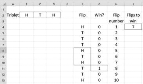
Our simulation in Excel consists of four sections: the chosen triplet, a sequence of coin flips, identification of when the triplet occurred in the sequence, and determination of the number of flips until observing the triplet. First, we set aside the three consecutive cells B2:D2 to contain the chosen triplet. Placing the triplet outside the code facilitates quick changes to the simulation. Second, we simulate a coin flip using the IF(RAND()>0.5, “H,” “T”) function in cells F4:F103. This generates 100 coin flips, sufficient to determine the number of flips to generate the chosen triplet. Third, we identify when the triplet is observed using an AND statement nested in an IF statement. The code for cell G11, which identifies the triplet in cells F8:F10, follows.$$\mathrm{G}11\mathrm{}=\mathrm{}\text{IF}\left(\text{AND}\left(\$\mathrm{B}\$2\mathrm{}=\mathrm{}\mathrm{F}8,\$\mathrm{C}\$2\mathrm{}=\mathrm{}\mathrm{F}9,\mathrm{}\$\mathrm{D}\$2\mathrm{}=\mathrm{}\mathrm{F}10\right),1,0\right)$$

Cell G11 returns a one if the cells F8:F10 contain the same sequence as cells B2:D2. Fourth, we determine how many flips occurred until the triplet was observed with a VLOOKUP function. The code in cell I4, which identifies when the triplet occurred and returns the flip number, follows.$$\mathrm{I}4\mathrm{}=\mathrm{}\text{VLOOKUP}\left(1,\mathrm{G}7:\mathrm{H}103,2,\text{FALSE}\right)-1$$

After building the simulation, we now use it to estimate the mean number of flips until observing each of the eight triplets. We randomly generate a large of games by repeatedly pressing the F9 button. The F9 button directs Excel to generate new random observations from all the RAND() function calls on the sheet. We cycle through each of the eight triplets, generating a large number of games, and calculating the mean number of flips until each triplet is observed. The strong law of large numbers tells us that the sample mean converges almost surely to the expected value. Sample sizes greater than 1000 typically yield estimates within one flip of the actual mean.

3.2 Monte Carlo Simulation in R

R provides another excellent environment in which to conduct a Monte Carlo simulation. Many college students, especially those in more mathematically rigorous disciplines, have experience either coding in R or in another language.

We conduct a Monte Carlo simulation in R to estimate the solution of the expected value problem with two user-defined functions, flip and sim.flip. The function flip takes a triplet and calculates how many coin flips are required to achieve the triplet. The function sim.flip executes the flip function a specified number of times. The R code for both functions follows below in Appendix A. The flip function takes the triplet as three arguments. The function then generates a sequence of three coin flips. The triplet is then compared to the sequence. If they match, the number of flips is returned and the function exits. If they do not match, another flip is generated. The process continues until the triplet is observed in the sequence. The sim.flip function takes the triplet and the number of games to simulate as arguments. The function calls the flip function the requested number of times and then calculates the simulated mean number of flips until observing the triplet.

After defining these two functions, we now utilize them to estimate the mean number of flips until observing each of the eight triplets. We cycle through each of the eight triplets, generating a large number of games, and calculating the simulated mean number of flips until each triplet is observed. Samples of size of 100,000 yield sample means mostly within 0.10 flips of the actual population means.

3.3 Closed-Form Solution

Deriving a closed-form solution for the expected number of coin flips until one sees a specific triplet (expected value problem) requires a level of mathematical maturity that not all college students possess. However, deriving these solutions not only provides precise answers but also yields unique insights into the expected value problem. As an example, we derive the expected number of flips until observing the triplet HTH.

Let X be the number of coin flips until HTH occurs for the first time. We want to compute $E(X).$

Consider the first flip of the coin. $E(X)$ is the weighted sum of the conditional expectations of X:(1) $$E\left(X\right)=E\left(X|H\right)P\left(H\right)+E\left(X|T\right)P\left(T\right).$$(1)

Notice that $E(X|T)=E(X)+1$, since one “restarts the counting” if the first flip is a T. Since $P(H)=P(T)=\frac{1}{2},$ then, we can rewrite E(X) in (1) as(2) $$E\left(X\right)=\frac{1}{2}E\left(X|H\right)+\frac{1}{2}\left[E\left(X\right)+1\right]=E\left(X|H\right)+1.$$(2)

We now turn our attention to computing $E(X|H)$. Consider the second flip of the coin. $E(X|H)$ is the weighted sum of conditional expectations of $X|H$:(3) $$E\left(X|H\right)=E\left(X|HT\right)P\left(T\right)+E\left(X|HH\right)P\left(H\right).$$(3)

Notice that $E(X|HH)=E(X|H)+1$, since one “restarts the counting with H” if the second flip is a H. Since $P(H)=$ $P(T)=\frac{1}{2},$ we can rewrite $E(X|H)$ in (3) as(4) $$E\left(X|H\right)=\frac{1}{2}E\left(X|HT\right)+\frac{1}{2}\left[E\left(X|H\right)+1\right]=E\left(X|HT\right)+1.$$(4)

We now turn our attention to computing $E(X|HT)$. Consider the third flip of the coin. $E(X|HT)$ is the weighted sum of conditional expectations of $X|HT$.(5) $$E\left(X|HT\right)=E\left(X|\mathit{HTH}\right)P\left(H\right)+E\left(X|\mathit{HTT}\right)P\left(T\right).$$(5)

We have that $E(X|\mathit{HTH})=3$, since you observed the triplet. Also, $E(X|\mathit{HTT})=E(X)+3$, since one “restarts the counting” if the third flip is a T. This allows us to rewrite $E(X|HT)$ as follows:(6) $$E\left(X|HT\right)=\frac{1}{2}3+\frac{1}{2}\left(E\left(X\right)+3\right)=\frac{1}{2}E\left(X\right)+3.$$(6)

Place the result from formula (6) into formula (4) to obtain(7) $$E\left(X|H\right)=\left[\frac{1}{2}E\left(X\right)+3\right]+1=\frac{1}{2}E\left(X\right)+4.$$(7)

Place the result from formula (7) into formula (2) to obtain$$E\left(X\right)=\left[\frac{1}{2}E\left(X\right)+4\right]+1=10$$

3.4 Intuition

Why do some triplets occur, on average, sooner than others do? The key is to consider what happens when a specific triplet fails to occur in the first three flips and where that leaves the sequence. Consider player A with triplet HHH. If the triplet fails on any of the first three flips (T, HT, or HHT), then player A starts again (i.e., player A will require at least three more flips to win). Now consider player B with triplet HTH. If the triplet fails on either the first or third flip (T or HTT), then player B starts again. However, if the triplet fails on the second flip (HH), then player B is one correct flip (the first head) into the triplet, needing just TH to win. Finally consider player C with triplet HHT. If the triplet fails on either the first or second flip (T or HT), then player C starts again. However, if the triplet fails on the third flip (HHH), then player C is two correct flips (the first two heads) into his triplet. Figure 2 shows these results.

Fig. 2 Number of flips into the triplet at failure. A triplet can fail at the first, second, or third flip in a sequence of three flips. At the time of failure, the triplet will require, at a minimum, one to three more flips before being observed.

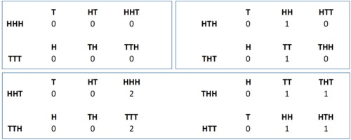
The triplets HHH (player A) and TTT always start again when the triplet fails. These two have an expected value of 14 flips. The triplets HTH (player B) and THT start again when they fail on the first or third flip, but are one flip into their sequence when they fail on the second flip. These two have an expected value of 10 flips. The triplets HHT (player C) and TTH start again when they fail in the first two flips, but are two flips into their sequence when they fail on the third flip. These two have an expected value of eight flips. The triplets THH and HTT start again when they fail on the first flip, but are one flip into their sequence when they fail on either the second or third flip. These two also have an expected value of eight flips. The eight triplets have three different expected values. Which of these three a triplet takes depends upon how far into their sequence the triplet is at failure.

4 The Superior Triplet Problem

Consider a simple game in which the students choose triplets, say A and B, and the student whose chosen triplet appears first wins a prize. We begin by asking the students which triplet they would choose when playing the game. Most students lack the intuition to see which triplets to prefer. However, after observing the results of Table 1, most will choose one of the four triplets with eight expected flips for their occurrence. We then ask them, in all possible pairings, which triplets are most likely to be observed first. Most will say that the triplet with a smaller expected number of flips until observation is more likely to be observed first. At this time, we find it useful to share the actual probabilities of observing triplet B before triplet A for all possible pairings shown in Table 2.

Table 2 Superior triplets (table).

	Player B
		TTT	TTH	THT	HTT	THH	HTH	HHT	HHH
Player A	TTT	–	1/2	3/5	3/5	3/5	7/12	7/10	1/2
	TTH	1/2	–	1/3	3/4	1/3	3/8	1/2	3/10
	THT	2/5	2/3	–	1/2	1/2	1/2	5/8	5/12
	HTT	1/8	1/4	1/2	–	1/2	1/2	2/3	2/5
	THH	2/5	2/3	1/2	1/2	–	1/2	1/4	1/8
	HTH	5/12	5/8	1/2	1/2	1/2	–	2/3	2/5
	HHT	3/10	1/2	3/8	1/3	3/4	1/3	–	1/2
	HHH	1/2	7/10	7/12	3/5	7/8	3/5	1/2	–

NOTE: The probability of observing triplet B before triplet A. Probabilities exceeding one half are shaded in gray, that is, superior triplets.

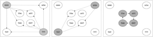
Students are often surprised to discover that for every triplet, there is at least one other triplet that is superior. In fact, two have five superior triplets, two have two superior triplets, and four have just one superior triplet. Students who learn visually often find it helpful to see these relationships displayed graphically (see Figure 3).

Fig. 3 Superior triplets (graph). If Player A selects a grayed triplet, any triplet connected by an arrow has greater than one-half probability of appearing before Player A’s triplet.

Before moving onto proving the results, we have the students return to playing the game, knowing now how likely they are to win in different settings. Practical experience helps reinforce which triplets are superior.

Next, we task the students with either estimating or deriving the probabilities of one triplet beating another, building on the work students did to solve the expected value problem. We describe below how to build the Monte Carlo simulations in Excel and R, derive the closed-form solution, and provide intuition to clarify the results.

4.1 Monte Carlo Simulation in Excel

We obtain a solution to the superior triplet problem from the Monte Carlo simulation in Excel shown below in Figure 4.

Fig. 4 Monte Carlo simulation in Excel-modified. The cells with borders (e.g., I4) identify cells whose code is explained in the article.

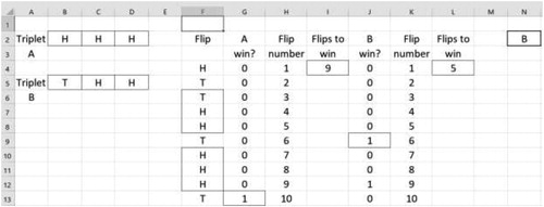
We modify our earlier simulation to compute probabilities of one triplet occurring before another in Excel. Our simulation in Excel now consists of five sections: the two triplets, a sequence of coin flips, identification of each triplet in the sequence, determination of the number of flips until observing each triplet, and determination of which triplet occurred first. First, we set aside the three consecutive cells B2:D2 and B5:D5 to contain the triplets. Again, placing the triplets outside the code facilitates quick changes to the simulation. Second, we simulate a coin flip using the RAND() function in cells F4:F103. This generates 100 coin flips, sufficient to determine a winner of the triplet game. Third, we identify when each triplet is observed using an AND statement nested within an IF statement. The code for cell G13, which identifies the first triplet (A) in cells F10:F12, and the code for cell J9, which identifies the second triplet (B) in cells F6:F8, follows.$$+\mathrm{G}13\mathrm{}=\mathrm{}\text{IF}\left(\text{AND}\left(\$\mathrm{B}\$2=\mathrm{F}10,\$\mathrm{C}\$2=\mathrm{F}11,\$\mathrm{D}\$2=\mathrm{F}12\right),1,0\right)+$$$$+\mathrm{J}9\mathrm{}=\mathrm{}\text{IF}\left(\text{AND}\left(\$\mathrm{B}\$5=\mathrm{F}6,\$\mathrm{C}\$5=\mathrm{F}7,\$\mathrm{D}\$5=\mathrm{F}8\right),1,0\right)\mathrm{}+$$

Fourth, we determine how many flips occurred until each triplet was observed with a VLOOKUP function. The code in cells I4 and L4, which identifies when each triplet occurred and returns the flip numbers, follows.$$\mathrm{I}4\mathrm{}=\mathrm{}\text{VLOOKUP}\left(1,\mathrm{G}7:\mathrm{H}103,2,\text{FALSE}\right)-1$$$$\mathrm{L}4\mathrm{}=\mathrm{}\text{VLOOKUP}\left(1,\mathrm{J}7:\mathrm{K}103,2,\text{FALSE}\right)-1$$

Fifth, we determine which of the two triplets occurred first with an IF statement. The code in cell K2, which compares the number of flips until each triplet is observed, follows.$$\mathrm{N}2\mathrm{}=\mathrm{}\text{IF}\left(\mathrm{I}4<\mathrm{L}4,"\mathrm{A}","\mathrm{B}"\right)$$

After modifying the simulation, we now use it to estimate the probability of winning with each triplet against each of the other seven triplets. We cycle through each of the 64 triplet pairs, generating a large number of games, and calculating the percentage of time each triplet was observed first. Borel’s law of large numbers tells us that the sample proportion converges to the population proportion. Samples of size 100,000 typically yield estimates within 0.01% of the actual probability. These calculations again provide an excellent opportunity to observe and discuss the relationship between sample size and convergence.

4.2 Monte Carlo Simulation in R

We conduct a second Monte Carlo simulation in R to compute probabilities of one triplet occurring before another (the superior triplet problem) with two additional user-defined functions, compare and sim.compare. The function compare takes two triplets and determines which occurs first in a sequence of simulated coin flips. The function sim.compare executes the compare function a specified number of times. The R code for both functions follows in Appendix A. The compare function takes the two triplets as arguments. The function then generates a sequence of three coin flips, again with the rbinom function. Both triplets are compared to the sequence. If either matches, that triplet is returned as the winner. If neither matches, another flip is generated. The process continues until one of the triplets is observed in the sequence. The sim.compare function takes the two triplets and the number of games to simulate as arguments. The function calls the compare function the requested number of times and stores the result in a vector.

After defining these two functions, we now utilize them to estimate the probability of winning with each triplet against each of the other seven triplets. We cycle through each of the 64 triplet pairs, generating a large number of games, and calculating the percentage of time each triplet was observed first.

4.3 Closed-Form Solution

In this section, we derive a closed form solution for the superior triplet problem—the probability that a selected triplet occurs before another one. Take two distinct triplets, A and B. We will find the probability that B occurs before A when flipping a fair coin. For example, take $A=\mathit{HHT}\wedge B=\mathit{HTT}$ triplets. Let X be the event that B occurs before A. We need to determine $P(X).$ Define the following probabilities:

• $P(X|HH)$ is the probability that B occurs before A, given that the first two flips were HH.

• $P(X|HT)$ is the probability that B occurs before A, given that the first two flips were HT.

• $P(X|TH)$ is the probability that B occurs before A, given that the first two flips were TH.

• $P(X|TT)$ is the probability that B occurs before A, given that the first two flips were TT.

We have(8) $$\ll \begin{array}{c}P\left(X\right)=P\left(X|HH\right)P\left(HH\right)+P\left(X|HT\right)P\left(HT\right)\\ \hspace{1em}+P\left(X|TH\right)P\left(TH\right)+P\left(X|TT\right)P\left(TT\right)\\ =\frac{1}{4}(P\left(X|HH\right)+P\left(X|HT\right)+P\left(X|TH\right)+P\left(X|TT\right))\end{array}$$(8) since $P(HH)=P(HT)=P(TH)=P(TT)=\frac{1}{4}.$

Each of these conditional probabilities of the equation above can be written as follows:(9.1) $$\begin{array}{c}P\left(X|HH\right)=P\left(X|\mathit{HHH}\right)P\left(H\right)+P\left(X|\mathit{HHT}\right)P\left(T\right)\\ =\frac{1}{2}(P\left(X|\mathit{HHH}\right)+P\left(X|\mathit{HHT}\right))\end{array}$$(9.1) (9.2) $$\begin{array}{c}P\left(X|HT\right)=P\left(X|\mathit{HTH}\right)P\left(H\right)+P\left(X|\mathit{HTT}\right)P\left(T\right)\\ =\frac{1}{2}\left(P\left(X|\mathit{HTH}\right)+P\left(X|\mathit{HTT}\right)\right)\end{array}$$(9.2) (9.3) $$\begin{array}{c}P\left(X|TH\right)=P\left(X|\mathit{THH}\right)P\left(H\right)+P\left(X|\mathit{THT}\right)P\left(T\right)\\ =\frac{1}{2}\left(P\left(X|\mathit{THH}\right)+P\left(X|\mathit{THT}\right)\right)\end{array}$$(9.3) (9.4) $$\begin{array}{c}P\left(X|TT\right)=P\left(X|\mathit{TTH}\right)P\left(H\right)+P\left(X|\mathit{TTT}\right)P\left(T\right)\\ =\frac{1}{2}\left(P\left(X|\mathit{TTH}\right)+P\left(X|\mathit{TTT}\right)\right)\end{array}$$(9.4)

Keeping in mind that X is the event that the triplet $B=\mathit{HTT}$ occurs before the triplet $A=\mathit{HHT}$, the eight conditional probabilities on the right sides of the above four equations (which are conditioned on the first three flips) can be written as(10.1) $$P\left(X|\mathit{HHH}\right)=P\left(X|HH\right)$$(10.1) (10.2) $$P\left(X|\mathit{HHT}\right)=0$$(10.2) (10.3) $$P\left(X|\mathit{HTH}\right)=P\left(X|TH\right)$$(10.3) (10.4) $$P\left(X|\mathit{HTT}\right)=1$$(10.4) (10.5) $$P\left(X|\mathit{THH}\right)=P\left(X|HH\right)$$(10.5) (10.6) $$P\left(X|\mathit{THT}\right)=P\left(X|HT\right)$$(10.6) (10.7) $$P\left(X|\mathit{TTH}\right)=P\left(X|TH\right)$$(10.7) (10.8) $$P\left(X|\mathit{TTT}\right)=P\left(X|TT\right)$$(10.8)

Using the expressions in (10.1)–(10.8) in the equations in (9.1)–(9.4) will give us:(11.1) $$P\left(X|HH\right)=\frac{1}{2}\left(P\left(X|HH\right)+0\right)=\frac{1}{2}P\left(X|HH\right)$$(11.1) (11.2) $$P\left(X|HT\right)=\frac{1}{2}\left(P\left(X|TH\right)+1\right)$$(11.2) (11.3) $$P\left(X|TH\right)=\frac{1}{2}\left(P\left(X|HH\right)+P\left(X|HT\right)\right)$$(11.3) (11.4) $$P\left(X|TT\right)=\frac{1}{2}\left(P\left(X|TH\right)+P\left(X|TT\right)\right)$$(11.4)

Solving these four equations for the four unknowns gives us:$$\begin{array}{c}P\left(X|HH\right)=0,\hspace{1em}P\left(X|HT\right)=\frac{2}{3},\\ P\left(X|TH\right)=\frac{1}{3},\hspace{1em}P\left(X|TT\right)=\frac{1}{3}.\end{array}$$

Therefore,$$\begin{array}{c}P\left(X\right)=\frac{1}{4}(P\left(X|HH\right)+P\left(X|HT\right)+P\left(X|TH\right)\\ \hspace{1em}+P\left(X|TT\right))=\frac{1}{3}.\end{array}$$

4.4 Intuition

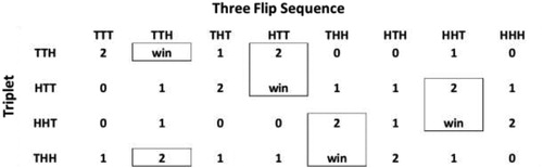
Most students are not surprised by the fact that a triplet with a larger expected value is never superior to a triplet with a smaller expected value. They do struggle to understand why one triplet is superior to another with the same expected value. We point out that the current sequence of flips in a game tends to favor one triplet over another. A superior triplet is one in which sequences, on average, favor it over the inferior triplet. Consider TTH and HTT. Both have an expected value of eight, but HTT is superior to TTH. The reason for HTT’s superiority becomes apparent when one compares the two triplets side by side across each of the eight possible three flip sequences (see Figure 5). Each triplet wins with one of the sequences, and is either zero, one, or two flips into their sequence after failing with one of the other seven. Compare where one triplet is when the other wins. TTH is two flips into its sequence when HTT wins, but HTT is only one flip into its sequence when TTH wins. HTT is superior because its winning sequence occurs at one of TTH’s best nonwinning sequences. In fact, this occurs for each superior triplet among the four triplets with an expected value of eight.

Fig. 5 The number of flips into a triplet’s sequence for each three flip sequence. A triplet is superior to the triplet above it (i.e., THH is superior to HHT) and TTH is superior to THH. The boxes show how each superior triplet wins when its inferior triplet is two flips into its sequence.

5 Closing Notes

Each of the three solutions provides different opportunities to explain the complexity of dependence to students. The Monte Carlo simulation in Excel provides an opportunity for the students to observe long sequences of flips. This helps them to develop an intuitive understanding of the independence of a flip from prior flips, the dependence of a triplet on prior flips, why some triplets have larger expected values than others, and why some are superior (as we have defined the term) to others. We have our students estimate the distributions of a flip and a triplet, given prior flips, from a long sequence of flips. These demonstrations help clarify the meaning of dependence and independence. We also have our students estimate the expected value a triplet and the percentage of time that one triplet occurs before another. These demonstrations allow the students to observe the empirical results of the expected value and superior triplet problems. The Monte Carlo simulation in R code provides an opportunity to observe and discuss the relationship between sample size and convergence. R handles large sample sizes much better than Excel, as one is not restricted to the dimensions of a spreadsheet. We have our students vary the sample size argument in both the functions sim.flip and sim.compare to allow them to observe how the sample means and proportions converge to the population means and proportions as the sample sizes increase. A common mistake that students make is to spend a considerable amount of time building the simulation and then quickly estimate the expected values with a small number of simulation runs. The closed form derivations provide an opportunity to observe and discuss the nested conditional probabilities needed to derive the expected value. Although not all students have the mathematical maturity to understand the derivations, they provide another level of understanding to those that do.

5 Appendix A:

R Code

flip<-function(a,b,c){
counter<-3
pick<-c(a,b,c)
t<-rbinom(n = 3, size = 1, prob = 0.5)
repeat{
if(all(t==pick)){
break
}
t[1]<-t[2]
t[2]<-t[3]
t[3]<-rbinom(n = 1, size = 1, prob = 0.5)
counter<-counter + 1
}
return(counter)
}

sim.flip<-function(n,a,b,c){
result<-numeric(n)
for(i in 1:n){
result[i]<-flip(a,b,c)
}
return(sum(result)/n)
}

compare<-function(a,b,c,d,e,f){
counter<-3
pick1<-c(a,b,c)
pick2<-c(d,e,f)
t<-rbinom(n = 3, size = 1, prob = 0.5)
repeat{
if(all(t==pick1)){
win<-0
break
}
if(all(t==pick2)){
win<-1
break
}
t[1]<-t[2]
t[2]<-t[3]
t[3]<-rbinom(n = 1, size = 1, prob = 0.5)
counter<-counter + 1
}
return(win)
}

sim.compare<-function(n,a,b,c,d,e,f){
result<-numeric(n)
for(i in 1:n){
result[i]<-compare(a,b,c,d,e,f)
}
return(result)

}

References

- Braun, J. W., White, B. J., and Craig, G. (2014), “R Tricks for Kids,” Teaching Statistics, 36, 7–12. DOI: 10.1111/test.12016.
- Degner, K. (2015), “Flipping Out: Calculating Probability With a Coin Game,” Mathematics Teaching in Middle School, 21, 244–247.
- GAISE College Report ASA Revision Committee (2016), “Guidelines for Assessment and Instruction in Statistics Education College Report,” available at http://www.amstat.org/education/gaise.
- Hodgson, T., and Burke, M. (2000), “On Simulation and the Teaching of Statistics,” Teaching Statistics, 22, 91–96. DOI: 10.1111/1467-9639.00033.
- Jamie, D. (2002), “Using Computer Simulation Methods to Teach Statistics: A Review of the Literature,” Journal of Statistics Education, 10, 1–16. DOI: 10.1080/10691898.2002.11910548.
- Kruskal, W. (1988), “Miracles and Statistics: The Casual Assumption of Independence,” Journal of the American Statistical Association, 83, 929–940.
- Maxwell, N. P. (1994), “A Coin-Flipping Exercise to Introduce the P-Value,” Journal of Statistics Education, 2, 1, DOI: 10.1080/10691898.1994.11910465.
- Miller, J., and Sanjurjo, A. (2018), “Surprised by the Hot Hand Fallacy? A Truth in the Law of Small Numbers,” Econometrica, 86, 2019–2047. DOI: 10.3982/ECTA14943.
- Morgan, L. A., and Morgan, F. W. (1984), “Personal Computers, p-Values, and Hypothesis Testing,” Mathematics Teacher, 77, 473–478.
- Popham, W. J., and Sirotnik, K. Q. (1992), Understanding Statistics in Education, Itasca, IL: F. E. Peacock Publishers.
- Sigal, M., and Chalmers, P. (2016), “Play It Again: Teaching Statistics With Monte Carlo Simulation,” Journal of Statistics Education, 24, 136–156. DOI: 10.1080/10691898.2016.1246953.
- Vaughan, T., and Berry, K. (2005), “Using Monte Carlo Techniques to Demonstrate the Meaning and Implications of Multicollinearity,” Journal of Statistics Education, 13, 1–9. DOI: 10.1080/10691898.2005.11910640.