Studying the Strength of Prediction Using Indirect Mixture Modeling: Nonlinear Latent Regression with Heteroskedastic Residuals

Abstract

We present a latent regression model in which the regression function is possibly nonlinear, and not necessarily smooth (e.g., a step function), and in which the residual variances are not necessarily homoskedastic. Heteroskedasticity is modeled by making the conditional (on the predictor) residual variance a (user-specified) function of the predictor. We use indirect mixture modeling to estimate the parameters by marginal maximum likelihood estimation, as proposed by Bock and Aitken (1981) in the context of item-response theory modeling and Klein and Moosbrugger (2000) in the context of structural equation modeling. We present a small simulation study to evaluate power and the consequences of model misspecification, and an illustration concerning neuroticism and extroversion. The model can be used to evaluate changes in the strength of the prediction as a function of the predictor.

Keywords:

• heteroskedasticity
• indirect mixture
• latent regression
• marginal maximum likelihood
• nonlinearity

In direct applications of finite mixture modeling, the aim is to identify latent classes (mixture components), which are amenable to substantive interpretation (e.g., Dolan, Schmittmann, Lubke, & Neale, 2005; Muthén, Khoo, Francis, & Boscardin, 2003; Schmittmann, Dolan, van der Maas, & Neale, 2005). In indirect applications, mixture modeling is used as a tool to obtain a flexible, tractable form of analysis (e.g., Bauer, 2005; Kelava, Nagengast, & Brandt, 2014; Moosbrugger, Schermelleh-Engel, Kelava, & Klein, 2009). For instance, finite mixture factor analysis has been used indirectly to accommodate nonnormality (Wall, Gua, & Amemiya, 2012), and directly to identify interpretable latent classes (Dolan & van de Maas, 1998; Lubke & Muthén, 2005). In this article, we use indirect mixture modeling to accommodate nonlinearity and heteroskedasticity in the latent regression model.

We consider the combination of nonlinearity and heteroskedasticity to be of substantive interest to model changes in the strength of prediction. For instance, consider the statement “Social isolation (SI) causes depression (D),” which can be formalized in terms of the linear regression of D on SI. The psychological shorthand narrative is intuitively appealing: the more isolated you are, the more likely you are to be depressed (Cacioppo, Hawkley, & Thisted, 2010). However, it is possible that at low, or even intermediate, levels of depression, depression is less strongly associated with social isolation. This variation in strength of the relationship might be due to heteroskedasticity (e.g., σ² [D|SI high] < σ²[D|SI low]), or due to variation in the value of the regression coefficient, β (e.g., β|SI high > β|SI low). The latter results in nonlinearity, whereas the former does not. However, both have a bearing on the strength of the regression relationship.

To accommodate nonlinearity, latent polynomial regression is often used. Two main approaches are the (latent) product-indicator approach and the distribution analytic approach (Moosbrugger et al., 2009). Within the product indicator approach latent nonlinearity is specified by including appropriate functions of the observed indicators (Bollen, 1995; Jaccard & Wan, 1996; Jöreskog & Yang, 1996; Kenny & Judd, 1984; Ping, 1996; Schumacker & Marcoulides, 1998). The product-indicator approach requires nonlinear constraints (but see Marsh, Wen, & Hau, 2004), and estimation suitable for nonnormality, given the nonnormality arising from the inclusion of product indicators. Within the distribution analytic approach, the model is estimated by conditioning on latent variables involved in the nonlinear regression terms. This can either be done by formulating the model as an indirect mixture (e.g., the latent moderated structural equation approach; Klein & Moosbrugger, 2000) or by approximating the nonnormal density function of the joint indicator vector (e.g., using quasi-maximum likelihood estimation; Klein & Muthén, 2007). A second indirect mixture approach to nonlinearity was developed by Bauer (2005; see also Pek, Sterba, Kok, & Bauer, 2009). Bauer proposed an exploratory regression model that approximates the nonlinear regression function by means of a weighted combination of linear regression models. This method requires specification of the number of components in the indirect mixture, not of the functional form of the nonlinear function (e.g., curvilinear, quadratic, exponential).

In the methods mentioned so far, heteroskedasticity, if any, is not modeled and not of substantive interest. Generally, in linear regression modeling, heteroskedasticity is viewed as an obstacle to correct statistical inference concerning regression coefficients, which can be addressed by iterated weighted least squares (Greene, 2011; Hooper, 1993) or by a correction of the standard errors (Huber, 1967; White, 1980). However, heteroskedasticity can be of theoretical interest in its own right. For instance, heteroskedasticity is important in the study of ability differentiation (Molenaar, Dolan, & van der Maas, 2011), genotype by environment interaction (Molenaar et al., 2013; van der Sluis, Dolan, Neale, Boomsma, & Posthuma, 2006), and personality (i.e., schematicity hypothesis; Molenaar, Dolan, & de Boeck, 2012). As mentioned earlier, here we are interested in heteroskedasticity (in combination with possible nonlinearity), as it has a bearing on the precision of prediction in the regression model.

Within the context of factor models and item-response theory (IRT) models, Molenaar and colleagues used marginal maximum likelihood (MML) estimation to model nonlinearity and heteroskedasticity (Molenaar et al., 2012; Molenaar et al., 2011; Molenaar, Dolan, & Verhelst, 2010; Molenaar, Dolan, Wicherts, & van der Maas, 2010). This approach is similar to that of Klein and Moosbrugger (2000) as it also exploits the fact that MML estimation in psychometric modeling can be cast in terms of constrained finite mixture modeling (see later).

In this article, we use the indirect mixture modeling approach to fit a nonlinear heteroskedastic latent regression model using MML estimation. In the model, both the regression coefficient and the latent residual variance are deterministic functions of the latent predictor. We show that various forms of heteroskedasticity can be accommodated using smooth or step functions. Similarly, various forms of nonlinearity can be considered including, but not limited to, polynomial functions or smooth functions. The outline of this article is as follows. We first present the formal indirect mixture model. Next, we discuss MML estimation of the model parameters. Then, we present the results of a simulation study to demonstrate the viability of the model in terms of parameter recovery, power, and the effect of misspecification. We apply the model to a real data set pertaining to personality. Finally, we conclude the article with a brief discussion.

THE INDIRECT MIXTURE MODEL TO TEST NONLINEARITY AND HETEROSKEDASTICITY

The Linear and Homoskedastic Case

We consider two instances of the latent linear regression model (see Figure 1). We assume that the normally distributed predictor variable (η_x) is latent with L indicators and that the dependent variable (η_y) is either observed (Figure 1 bottom) or latent with K indicators (Figure 1 top). We assume the dependent variable (η_y) to be normal conditional on the predictor (η_y). The number of indicators is arbitrary but assumed to be sufficient to avoid problems of identification. In matrix notation, the model for the L-dimensional vector of predictor indicators, denoted by x, is given by

(1) $\mathbf{x}={\nu }_{\mathbf{x}}+{\lambda }_{\mathbf{x}}{\eta }_{\mathbf{x}}+{\epsilon }_{\mathbf{x}},$(1)

FIGURE 1  Regression models with four predictor and four dependent indicators (top) or one dependent (bottom).

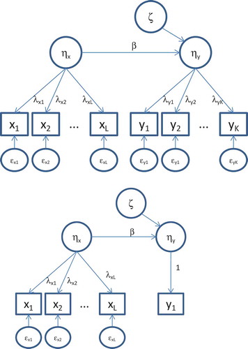
where ν_x is the L-dimensional vector of intercepts, λ_x is an L-dimensional vector of factor loadings, η_x is the 1 × 1 vector of the latent predictor (i.e., η_x = [η_x]), and ε_x is the L-dimensional vector of residuals. Next, the model for the K-dimensional vector of dependent latent variable indicators, denoted by y, given K > 1, is given by

(2) $y={\nu }_y+{\lambda }_y{\eta }_y+{\epsilon }_y,$(2)

with the parameters defined analogously. The preceding model reduces to y = ν_y + η_y if K = 1, as here the variable y features as the observed dependent. In the standard linear homoskedastic model, the latent dependent variable is regressed on the latent predictor variable as follows:

(3) ${\eta }_{\mathbf{y}}=\mathbf{B}{\eta }_{\mathbf{x}}+\zeta \mathbf{,}$(3)

where B is a 1 × 1 matrix containing the regression coefficient β, and ζ is a 1 × 1 matrix containing the latent residual ζ with variance σ_ζ². Homoskedasticity implies that the variance of ζ is constant over the range of η_x.

The Nonlinear and Heteroskedastic Case

We generalize the latent linear regression model to accommodate nonlinearity and heteroskedasticity simultaneously by making the regression coefficient β and the residual variance σ_ζ² a function of the predictor η_x:

(4) $\beta ={\mathrm{f}}_{\beta }({\eta }_{\mathrm{x}}),$(4)

and

(5) ${{\sigma }_{\zeta }}^2={\mathrm{f}}_{\zeta }({\eta }_{\mathrm{x}}).$(5)

The choice of the functions f_β(.) and f_ζ(.) is arbitrary, and not limited to smooth functions. An obvious smooth function is the r-degree polynomial regression:

(6) $\beta ={\mathrm{f}}_{\beta }({\eta }_{\mathrm{x}})={\gamma }_0+{\gamma }_1{\eta }_{\mathrm{x}}+{\gamma }_2{{\eta }_{\mathrm{x}}}^2+\dots +{\gamma }_{\mathrm{r}}{{\eta }_{\mathrm{x}}}^{\mathrm{r}}$(6)

where the model reduces to standard linear regression if γ_i = 0 (i = 1, …, r). As an example of a discrete function, consider a three-step function:

(7) $\begin{array}{rl}& \beta \hspace{0.17em}={\mathrm{f}}_{\beta }({\eta }_{\mathrm{x}})={\mathrm{k}}_0+{\mathrm{k}}_1\mathrm{i}\mathrm{f}{\eta }_{\mathrm{x}}\le -c\\ & {\mathrm{k}}_0\mathrm{i}\mathrm{f}-c<{\eta }_{\mathrm{x}}<c\\ & {\mathrm{k}}_0+{\mathrm{k}}_2\mathrm{i}\mathrm{f}{\eta }_{\mathrm{x}}\ge c\end{array}$(7)

where c is a chosen, fixed threshold value. To model heteroskedasticity of the latent residual, we could use an rth order polynomial function:

(8) ${{\sigma }_{\zeta }}^2={\mathrm{f}}_{\zeta }({\eta }_{\mathrm{x}})=\mathrm{e}\mathrm{x}\mathrm{p}({\varphi }_0+{\varphi }_1{\eta }_{\mathrm{x}}+{\varphi }_2{{\eta }_{\mathrm{x}}}^2+\dots +{\varphi }_{\mathrm{r}}{{\eta }_{\mathrm{x}}}^{\mathrm{r}})$(8)

or equivalently

(9) $\text{log}({\sigma }_{\zeta })=\text{log}({\text{f}}_{\zeta }({\eta }_{\text{x}}))={\varphi }_0+{\varphi }_1{\eta }_x+{\varphi }_2{\eta }_x+\dots +{\varphi }_r{\eta }_{\text{x}},$(9)

where the intercept ϕ₀ accounts for the latent residual, which is independent of the predictor η_x. In addition, ϕ_s (s = 1, …, r) are the heteroskedasticity parameters that account for the residual variance as a function of the predictor η_x. As in the case of the regression coefficient, other (discrete) functions can be chosen, such as the step function; for example,

(10) $\begin{array}{c}{{\sigma }_{\zeta }}^2={\mathrm{f}}_{\zeta }\left({\eta }_{\mathrm{x}}\right)={\xi }_0+{\xi }_1\mathrm{i}\mathrm{f}{\eta }_{\mathrm{x}}\le -\mathrm{c},\\ {\xi }_0\mathrm{i}\mathrm{f}\ge -\mathrm{c}<{\eta }_{\mathrm{x}}<\mathrm{c}\\ {\xi }_0+{\xi }_{2}if{\eta }_x\ge \hspace{0.17em}c.\end{array}$ (10)

The step function can be used in an exploratory analysis of heteroskedasticity in the extreme of the η_x distribution, where the choice of c is arbitrary (e.g., setting the threshold c to equal 1 SD; see the illustration later).

Parameter Estimation

Equations 1 through 5 represent the extended nonlinear latent regression model with heteroskedastic residuals. This model can be fitted by means of MML estimation (Bock & Aitkin, 1981; Klein & Moosbrugger, 2000; Molenaar et al., 2010), in which we condition on η_x and use Gauss–Hermite quadrature (Stroud & Secrest, 1966) to approximate the integral in the log-marginal likelihood.

To facilitate parameter estimation, we reformulate the models in Figure 1 into an equivalent specification, which is displayed in Figure 2. Specifically, given the model for the indicators of η_x in Equation 1, the conditional mean vector of the x indicators is given by μ_x|η_x = ν_x + λ_xη_x, and the conditional covariance matrix is given by Σ_x|η_x = Θ_x. When considering both nonlinearity and heteroskedasticity in the latent regression of η_y on η_x the model for the indicator vector of η_y conditional on η_x, is defined as y|η_x = ν_y + λ_y f_β(η_x) η_x + λ_y ζ + ε_y, where f_β(η_x) is specified as discussed earlier. In the case of a second-order polynomial, we have f_β(η_x) = γ₀+ γ₁η_x; that is,

$\begin{array}{c}\mathbf{y}|{\eta }_{\mathrm{x}}={\nu }_{\mathrm{y}}+{\lambda }_{\mathrm{y}}({\gamma }_0+{\gamma }_1{\eta }_{\mathrm{x}}){\eta }_{\mathrm{x}}+{\lambda }_{\mathrm{y}}\zeta +{\epsilon }_{\mathrm{y}}=\\ ={\nu }_{\mathrm{y}}+{\lambda }_{\mathrm{y}}({\gamma }_0{\eta }_{\mathrm{x}}+{\gamma }_1{{\eta }_{\mathrm{x}}}^2)+{\lambda }_{\mathrm{y}}\zeta +{\epsilon }_{\mathrm{y}},\end{array}$

FIGURE 2  Regression models with four predictor and four dependent indicators (top) or one dependent (bottom) in an equivalent (to Figure 1) specification. Note that β_k* = β × λ_yk where k = 1, …, K.

which reveals the quadratic nature of the regression model.

The vector of the conditional means of the dependent indicators is defined as μ_y|η_x = ν_y + λ_y f_β(η_x) η_x. The model-implied conditional covariance structure depends on the f_ζ (η_x), as follows: Σ_y|η_x = λ_y[f_ζ(η_x)]λ_y^t + Θ_y, where, for instance, f_ζ(η_x) = exp (ϕ₀ + ϕ₁η_x). To formulize the MML function we stack the indictor vectors of the predictor and dependent latent variable, x and y, into the vector z. In addition, the conditional mean vector of x and y is stacked into ${\mu }_{{\eta }_{\mathrm{x}}}$ and the conditional covariance matrix is the block matrix $\sum {\eta }_{\text{x}}$. Then, the conditional distribution of the data of subject i, z_i, is defined as

$h\left(z_i\text{|}{\eta }_{\text{x}},\tau \right)={\left(2\pi \right)}^{-M/2}{\left|\sum {\eta }_{\text{x}}\right|}^{-\frac{1}{2}}\text{exp}\left(-\frac{1}{2}{\left(z_i-{\mu }_{{\eta }_{\text{x}}}\right)}^{\prime }{\left[\sum {\eta }_{\text{x}}\right]}^{\text{-1}}\left(z_i\text{-}{\mu }_{{\eta }_{\text{x}}}\right)\right).$

By integrating out η_x, we obtain the marginal density of the observed variables for subject i

$k\left({\mathbf{z}}_i|\tau \right)=\underset{-\mathrm{\infty }}{\overset{\mathrm{\infty }}{\int }}h\left({\mathbf{z}}_i|{\eta }_{\mathrm{x}},\tau \right)\times \phi \left({\eta }_{\mathrm{x}}\right)d{\eta }_{\mathrm{x}},$

where $\phi \left({\eta }_{\mathrm{x}}\right)$ is a standard normal density function. Approximating the log of this density using Gauss–Hermite quadratures, we obtain

(11) $\mathrm{l}\mathrm{o}\mathrm{g}L\left(\tau |\mathbf{z}\right)\approx \sum _{i=1}^M\mathrm{l}\mathrm{o}\mathrm{g}\left(\sum _{q=1}^Q{W}_q^{\ast }\times h\left({\mathbf{z}}_{\mathbf{i}}|N_q^{\ast },\tau \right)\right),$(11)

where M is the number of subjects and τ is the parameter vector. In addition, N*_q = $\sqrt{2}$N_q and W*_q = $\frac{1}{\sqrt{\pi }}$ W_q where N_q and W_q are the Q nodes and weights (q = 1, …, Q), respectively of the Gauss–Hermite quadrature approximation. Note that 0 < W*_q < 1 and ${\displaystyle {\sum }_{q=1}^Q{W}_q^{*}=1}$, so that the log-marginal likelihood function, ${\displaystyle {\sum }_{q=1}^Q{W}_q^{*}\times h\left(z_i\text{|}{N}_q^{*},\tau \right)}$ has the form of a Q-component mixture distribution with the weights featuring as mixing proportions, and $h\left({\mathbf{z}}_{\mathbf{i}}|N_q^{\ast },\tau \right)$ featuring as the qth mixture component distribution. The model as defined earlier is implemented in OpenMx (Boker et al., 2011) within the R program (R Development Core Team, 2012).¹

SIMULATION STUDY

We explored the viability of this model by means of a small simulation study, in which we considered parameter recovery, power, and the effects of misspecification. We limited the simulation study to the second-order polynomial nonlinearity model and the second-order polynomial heteroskedasticity model, as defined in Equations 6 and 8. To make the relevant comparisons, we considered four instances of the model: the full model (i.e., the model with the regular regression parameters γ₀, ϕ_0, and the nonlinearity parameter γ₁, and heteroskedasticity parameter ϕ₁); the heteroskedasticity model (i.e., the model with parameters γ₀, ϕ₀, and ϕ₁); the nonlinearity model (i.e., the model with parameters γ₀, ϕ_0, and γ₁); and the basic model (i.e., the standard regression model with only parameters γ₀, ϕ₀). We denote these models as FULL, NON-L, HETERO, and BASIC, respectively.

Setting

We set the number of indicators of the latent predictor (η_x) to equal L = 4, and the number of indicators of the latent dependent variable (η_y) K = 4 or K = 1 (given K =1, η_y is simply equal to the dependent y). To fit the models, we used the following identifying (scaling) constraints; in each model the variance of η_x was fixed to 1. Additionally, given K = 4, the first factor loading of η_y was fixed to 1. To generate data, we set all 4 factor loadings associated with η_x to equal .5 and the factor loadings associated with η_y to equal 1. We fixed all latent variable means (i.e., E[η_x], E[η_y]) to equal zero, consistent with the data generating model. We set the variances of ε_x to equal .5 for all predictor indicators, and the variances of ε_y to equal 1 (but zero in the case of K = 1). Next, we set the baseline regression parameter (γ₀) to equal .4, and the baseline residual term (ϕ₀) to equal (±) .29, depending on whether the residual variance increased or decreased with the predictor.

To evaluate parameter recovery, power, and effects of misspecification of the model, we simulated data under the NON-L, HETERO, or FULL model, for both K = 4 and K = 1. Prior to the simulation study, we established the number of quadrature points needed for accurate estimation, and checked the Type I error rate. We found that 25 points were sufficient and we established that the empirical Type I error rate was equal to the nominal α (results available on request). We varied the values of the parameters of interest to be either small, medium, or large, and either positive or negative (i.e., γ₁ = ±.1; γ₁ = ±.15; γ₁ = ±.2, and ϕ₁ ≈ ±.22; ϕ₁ ≈ ±.31; ϕ₁ ≈ ±.40). Figure 3 depicts the effects. The upper half shows the simulated nonlinearity effects and the lower half shows the simulated heteroskedasticity effects. In the simulation we used all possible combination of effects (i.e., one or two effects present, positive or negative). This scheme led to 24 different parameter settings for both K = 4 and K = 1. We set the sample size to N = 300 and conducted 1,000 replications per parameter setting.

FIGURE 3  Overview of simulated effects. Top left and top right: nonlinearity of the regression relationship (e.g., top left γ₀ = .4, γ₁ = .1, .15, or .20, where β = g₀ + g₁*ηx and E[η_y|η_x] = β*η_x = γ₀*η_x+ γ₁*η_x²; see Equation 6). Bottom left and bottom right: heteroskedastic residual variance as function of η_x (e.g., bottom right ϕ₀ = .29, ϕ₁ = .22, .31, or .40, where the residual variance σ_ζ²|η_x = exp[ϕ₀ = ϕ₁*η_x]; see Equation 8).

RESULTS

Parameter Recovery

To check parameter recovery, we calculated the means and the standard deviations of the parameter estimates obtained under the true (data generating) model. Tables 1 through 3 show the means and standard deviations of the estimates obtained using the three models. Generally, the parameter values are recovered correctly. The parameter estimates pertaining to the residual variance (ϕ₀, ϕ₁) are slightly biased. However, the differences are negligible in the light of the standard deviations of the estimates. For instance, in Table 2, given K = 1, the expected value of ϕ₀ is .29 (in absolute value) and the mean estimated values vary between .27 and .31 (in absolute value), with a standard deviation of about .09. The estimates of the parameter pertaining to the regression function are accurate.

TABLE 1 Mean and Standard Deviations of Parameter Estimates Given K = 1 and K = 4 Dependent Variable Indicators, Given Nonlinearity

		K = 1			K = 4
Effect	Direction	γ0	ϕ0	γ1	γ0	ϕ0	γ1
Small		.40	−.29	(–).10	.40	−.29	(–).10
	γ1 < 0	.40(.06)	−.30(.09)	−.10(.05)	.40(.07)	−.31(.17)	−.10(.05)
	γ1 > 0	.40(.06)	−.30(.09)	.10(.05)	.40(.07)	−.32(.17)	.10(.05)
Medium				(–).15			(–).15
	γ1 < 0	.40(.06)	−.31(.09)	−.15(.05)	.40(.07)	−.31(.17)	−.15(.05)
	γ1 > 0	.40(.06)	−.30(.09)	.15(.05)	.40(.07)	−.30(.17)	.15(.05)
Large				(–).20			(–).20
	γ1 < 0	.40(.06)	−.30(.09)	−.20(.05)	.40(.07)	−.31(.17)	−.20(.05)
	γ1 > 0	.40(.06)	−.30(.09)	.20(.05)	.40(.07)	−.30(.17)	.20(.05)

Note. The true model (denoted NON-L) was fitted. Results are based on 1,000 replications (n = 300 per replication).

TABLE 2 Mean and Standard Deviations of Parameter Estimates Given K = 1 and K = 4 Dependent Variable Indicators, Given Heteroskedasticity

		K = 1			K = 4
Effect	Direction	γ0	ϕ0	ϕ1	γ0	ϕ0	ϕ1
Small		.40	(–).29	(–).22	.40	(–).29	(–).22
	ϕ1 < 0	.40(.06)	−.30(.09)	−.22 (.10)	.40(.07)	−.32(.17)	−.23(.13)
	ϕ1 > 0	.40(.08)	.27(.08)	.23(.10)	.40(.09)	.27(.14)	.23(.11)
Medium				(–).31			(–).31
	ϕ1 < 0	.40(.06)	−.31(.09)	−.31 (.10)	.40(.07)	−.31(.17)	−.30(.13)
	ϕ1 > 0	.40(.08)	.27(.09)	.31 (.10)	.40(.09)	.27(.14)	.31(.11)
Large				(–).41			(–).41
	ϕ1 < 0	.40(.06)	−.30(.09)	−.41(.10)	.40(.07)	−.32(.18)	−.40(.13)
	ϕ1 > 0	.40(.08)	.27(.09)	.40(.10)	.40(.09)	.27(.14)	.41(.12)

Note. The true model (denoted Hetero) was fitted. Results are based on 1,000 replications (n = 300 per replication).

Power

We evaluated the power of the likelihood ratio test to detect various effects. Given either nonlinearity or heteroskedasticity, we fitted the true data generating model (either NON-L or HETERO) and the alternative BASIC model. The likelihood ratio was based on minus twice the difference in likelihood values (BASIC vs. NON-L or HETERO; i.e., 1 df test). Given both effects, we fitted the true model (FULL) and the BASIC model. The likelihood ratio was based on minus twice the difference in likelihood values (BASIC vs. FULL; i.e., 2 df test). Table 4 contains the empirical power estimates based on 1,000 replications. Given medium effect sizes (i.e., ϕ₁ = ±.31 and γ₁ = ±.15), the power (df  = 2, α = .05) to detect both effects simultaneously is good (power = .89 or better). The power to detect heteroskedasticity (ϕ₁ ≠ 0) or nonlinearity (γ₁ ≠ 0) is sufficient (i.e., 1 df tests) given median effect sizes with power varying between .83 and .97 (γ₁ = ±.15) and .69 and .90 (ϕ₁ = ±.31). Given small effect sizes (i.e., ϕ₁ = ±.22 and γ₁ = ±.1) the 1 df tests are appreciably lower (ranging from .46–.68 to detect heteroskedasticity, ranging from .54–.63 to detect heteroskedasticity). Similarly, power of the 2 df tests is insufficient given small effects (ranging from .59–.87). Clearly N = 300 is too small a sample size to detect these effects with adequate power.

TABLE 3 Mean and Standard Deviations of Parameter Estimates Given K = 1 and K = 4 Dependent Variables Indicators, Given Nonlinearity and Heteroskedasticity

		K = 1			K = 4
Effect	Direction	γ0	ϕ0	γ1	ϕ1	γ0	ϕ0	γ1	ϕ1
Small		.40	−.29	(–).10	−.22	.40	−.29	(–).10	−.22
	γ1 < 0 ϕ1 < 0	.40(.06)	−.31(.10)	−.10(.05)	−.22(.10)	.40(.07)	−.32(.17)	−.10(.05)	−.22(.13)
	γ1 > 0 ϕ1 < 0	.40(.06)	−.31(.09)	.10(.05)	−.22(.10)	.40(.07)	−.32(.17)	.10(.05)	−.22(.13)
			.29	(–).10	.22		.29		.22
	γ1 > 0 ϕ1 > 0	.40(.08)	.27(.09)	.10(.06)	.23(.10)	.40(.09)	.26(.14)	.10(.06)	.23(.11)
	γ1 < 0 ϕ1 > 0	.40(.08)	.27(.09)	−.10(.06)	.23(.10)	.40(.09)	.26(.14)	−.10(.06)	.23(.13)
Medium			−.29	(–).15	−.31		−.29	(–).15	−.31
	γ1 < 0 ϕ1 < 0	.40(.07)	−.31(.10)	−.15(.05)	−.31(.10)	.40(.07)	−.32(.17)	−.15(.05)	−.31(.13)
	γ1 > 0 ϕ1 < 0	.40(.07)	−.31(.10)	.15(.05)	−.32(.05)	.40(.08)	−.32(.17)	.15(.05)	−.31(.13)
			.29	(–).15	.31		.29	(–).15	.31
	γ1 > 0 ϕ1 > 0	.40(.08)	.27(.09)	.15(.06)	.31(.10)	.41(.09)	.26(.14)	.15(.06)	.31(.11)
	γ1 < 0 ϕ1 > 0	.40(.08)	.27(.09)	−.15(.06)	.31(.10)	.40(.09)	.26(.14)	−.15(.06)	.31(.12)
Large			−.29	(–).20	−.41		−.29	(–).20	−.41
	γ1 < 0 ϕ1 < 0	.40(.08)	−.31(.17)	−.20(.05)	−.40(.10)	.40(.08)	−.32(.17)	−.20(.06)	−.41(.13)
	γ1 > 0 ϕ1 < 0	.40(.07)	−.31(.10)	.20(.05)	−.41(.12)	.40(.08)	−.31(.17)	.20(.06)	−.40(.14)
			.29	(–).20	.41		.29	(–).20	.41
	γ1 > 0 ϕ1 > 0	.40(.09)	.27(.09)	.20(.07)	.40(.10)	.40(.09)	.26(.14)	.20(.07)	.41(.12)
	γ1 < 0 ϕ1 > 0	.40(.08)	.27(.09)	−.20(.06)	.40(.11)	.40(.09)	.26(.14)	−.19(.07)	.41(.12)

Note. The true model (denoted Full) was fitted. Results are based on 1,000 replications (n = 300 per replication).

TABLE 4 Empirical Power to Detect Effects Given α = .05; 1 df Test (γ₁ ≠ 0 or ϕ₁ ≠ 0) and 2 df Test (γ₁ ≠ 0 and ϕ₁ ≠ 0), Given K = 1 and K = 4 Dependent Variable Indicators

Effect size	Direction	K = 1	K = 4
Small	γ1 < 0	.63	.55
	γ1 > 0	.61	.54
Medium	γ1 < 0	.89	.86
	γ1 > 0	.83	.97
Large	γ1 < 0	.98	.97
	γ1 > 0	.99	.97
Small	ϕ1 < 0	.67	.46
	ϕ1 > 0	.68	.55
Medium	ϕ1 < 0	.89	.69
	ϕ1 > 0	.90	.82
Large	ϕ1 < 0	.99	.91
	ϕ1 > 0	.99	.95
Small	γ1 < 0, ϕ1 < 0	.87	.75
	γ1 > 0, ϕ1 < 0	.79	.69
	γ1 > 0, ϕ1 > 0	.71	.63
	γ1 < 0, ϕ1 > 0	.66	.59
Medium	γ1 < 0, ϕ1 < 0	.99	.97
	γ1 > 0, ϕ1 < 0	.97	.95
	γ1 > 0, ϕ1 > 0	.95	.93
	γ1 < 0, ϕ1 > 0	.91	.89
Large	γ1 < 0, ϕ1 < 0	1	1
	γ1 > 0, ϕ1 < 0	1	1
	γ1 > 0, ϕ1 > 0	1	.99
	γ1 < 0, ϕ1 > 0	.99	.98

Note. Results are based on 1,000 replications (n = 300 per replication).

The 2 df tests have lower power if the effects are opposite effect (e.g., negative nonlinearity and positive heteroskedasticity). For instance, given small effects and K = 1, the power is .87 and .71 given consistent effects, and .79 and .66 given opposite effects (see Table 4 rows 13–16). Interestingly, this finding is consistent with the effects on the unconditional distribution of the data. Specifically, heteroskedasticity and nonlinearity consistently give rise to nonnormality, as evaluated using the Shapiro–Wilks test (results available on request). However, when both effects are present in opposite directions, nonnormality is harder to detect, which suggests that opposite effects on the distribution appear to cancel out. This suggests that apparent normality per se does not rule out the presence of heteroskedasticity in combination with opposite-effect nonlinearity.

Misspecification

We considered misspecified models to gauge the effect of the misspecification on the other parameters. We focused on the effects of the misspecification (dropping a parameter) on the other parameters as we wanted to establish the bias in the other parameters that this causes. We do not consider the effect on the goodness of fit per se as the results in Table 4 address this issue (in terms of power). We simulated data using three data generating models with either one effect (HETERO or NON-L), or both effects (FULL) present. We fitted misspecified models, which excluded these effects, as shown in Table 5. We simulated 1,000 data sets with the medium effect sizes for both K = 4, and K = 1 with positive heteroskedasticity and positive nonlinearity.

TABLE 5 Parameter Estimates in Misspecified Models, Given K = 1 or K = 4 Dependent Variable Indicators

		K = 1			K = 4
True Model	Fitted Model	γ0	ϕ0	γ1	ϕ1	γ0	ϕ0	γ1	ϕ1
HETERO		.40	−.29	.00	−.31	.40	−.29	.00	−.31
	BASIC	.40(.06)	−.25(.09)	−.03(.05)		.39(.07)	−.26(.17)	−.02(.05)
	NON-L	.40(.06)	–.27(.09)			.40(.07)	–.27(.17)
NONL		.40	−.29	.15	.00	.40	−.29	.15	.00
	BASIC	.40(.06)	−.24(.09)		.06(.10)	.40(.07)	−.25(.17)		−.04(.12)
	HETERO	.38 (.06)	–.25(.09)			.389 (.07)	–.25(.17)
FULL		.40	−.29	.15	−.31	.40	−.29	.15	−.31
	BASIC	.40(.06)	−.20(.09)	.13(.05)	−.23(.10)	.40(.07)	−.20(.17)	.13(.05)	−.26(.13)
	HETERO	.45(.06)	–.24(.09)			.45(.08)	–.25(.17)
	NON-L	.39(.06)	–.23(.09)			.39(.07)	–.25(.17)

Note. Results are based on 1,000 replications (n= 300 per replication).

We limit our discussion to the K = 1 condition, as the K = 4 results are similar. First, we consider the results obtained when the misspecified models were fit to data generated using the HETERO model (i.e., ϕ₁ ≠ 0, γ₁ = 0). In the BASIC model (i.e., fixing ϕ₁ to zero), the variance parameter ϕ₀ is somewhat biased (–.25 vs. –.29), as is to be expected. The results of fitting the NON-L model (ϕ₁ fixed to 0, and γ₁ estimated), demonstrates that γ₁ is hardly affected by the misspecification: –.03 (SD = .05) versus 0. Considering data generated under the NON-L model (i.e., ϕ₁ = 0, γ₁ ≠ 0), we find that fitting the BASIC model (i.e., ϕ₁ fixed to zero) results in a bias in the variance parameter ϕ₀ (–.24 vs. –.29). Fitting the HETERO model (i.e., ϕ₁ ≠ 0, γ₁ = 0) demonstrates that ϕ₁ is hardly affected by the misspecification (estimate = .06; SD = .10), but that γ₀ is slightly biased (.38 vs. .40). Overall misspecification could result in appreciable bias. However, the misspecification of heteroskedasticity (ϕ₀ = 0 and γ₁ ≠ 0 rather than ϕ₁ ≠ 0 and γ₁ = 0) produced little bias in the regression parameters (γ₁ is estimated close to its true value of 0), and vice versa. This suggests that the parameter sets {γ₀, γ₁} and {ϕ₀, ϕ₁} are relatively independent.

ILLUSTRATION

Data

We fitted the model to a subset of items from the Big Five Personality questionnaire 5PFT (Elshout & Akkerman, 1975). The 5PFT consists of five scales, each including 14 items measured with 7-point Likert scales. The data were obtained from Smits, Dolan, Vorst, Wicherts, and Timmerman (2011), and were collected in a sample of first-year psychology students in the Netherlands between 1982 and 2007. Smits et al. (2011) demonstrated that the 5PFT dimensions correspond to the five dimensions of the NEO PI (Costa & McCrae, 1985). We analyzed the data of the male students (N = 2,764) 18 to 25 years old. We created two subsamples of n = 1,382, a discovery and a replication sample.

Based on item reliability, we selected a subset of four predictors and four observed outcome items from the Neuroticism and the Extroversion scale. The reliabilities (Cronbach’s α) of these small scales are .78 (Extroversion) and .84 (Neuroticism) in the first sample, and .78 (Extroversion) and .85 (Neuroticism) in the second sample. The means and the standard deviations in the two samples are shown in Table 6.

TABLE 6 Overview of Means and Standard Deviations in the Two Samples Used in the Illustration

	Sample 1 (n = 1,382)		Sample 2 (n = 1,382)
	M	SD	M	SD
Age	20.59	1.87	20.6	1.88
yE1	4.44	1.52	4.46	1.52
yE2	4.10	1.59	4.15	1.57
yE3	4.33	1.53	4.42	1.48
yE4	4.56	1.48	4.59	1.48
yN1	3.36	1.42	3.33	1.39
yN2	3.18	1.62	3.12	1.62
yN3	3.70	1.51	3.63	1.51
yN4	3.10	1.56	3.00	1.50

Note. y_E1 to y_E4 are the indicators of extraversion; y_N1 to y_N4 are the indicators for neuroticism.

Models

To illustrate the model, we used two different functions to model heteroskedasticity and nonlinearity. First, we used the first-order polynomial function using the regression parameters γ₀, γ₁, and heteroskedasticity parameters ϕ₀, ϕ₁. Second, we used the step function using the parameters κ₀, κ_1, κ₂ (see Equation 7) for the stepwise regression, and stepwise heteroskedasticity parameters ξ₀, ξ₁, ξ₂ (see Equation 10). For the step function, the cutoff points were set at −1 SD and +1 SD of the item scores. We first fitted the full models in which both effects were present (denoted either S-FULL or L-FULL), and we then fitted the nonlinearity model (NON-L) and the heteroskedasticity model (HETERO). Finally, we fitted the standard latent regression model. In total, we fitted seven different models: BASIC, L_HETERO, L_NON-L, L_FULL, and S_HETERO, S_NON-L, S_FULL. In the polynomial and the step function model, we applied the likelihood ratio test to determine whether we could drop the heteroskedasticity, the nonlinearity parameter, or both by making the following comparisons. For both the polynomial model and the step function model we first compared the FULL model with the BASIC model using an omnibus test (both effects). Second, we compared the FULL model with the HETERO and NON-L model. Finally, we compare the HETERO and NON-L model with the BASIC model. Given the exploratory nature of these analyses, we adopted an α of .05 and used the replication sample to replicate results obtained in the discovery sample. To determine which model best fit the data, we compared the overall fit of the models using Akaike’s information criteria (AIC). All models were fitted to the Neuroticism and Extroversion data (discovery sample and the replication sample) in OpenMx (Boker et al., 2011) by maximizing the likelihood function given in Equation 11.

RESULTS

Results Using the Polynomial Model

Table 7 gives an overview of the fit measures and likelihood ratio tests obtained in fitting the models to the two data sets. We found that in the polynomial model the omnibus test of both effects (nonlinearity and heteroskedasticity) was significant in the discovery sample and replicated in the replication sample: comparison of L_FULL with BASIC, discovery sample, χ²(2) = 11.73, p = .0028; replication sample, χ²(2) = 15.69, p = .0004. Additional comparisons showed that the nonlinearity parameter γ₁ was not significant: L_FULL versus L_HETERO model, discovery sample 1, χ²(1) = .35, p = .55; replication sample, χ²(1) = 1.21, p = .27; whereas the heteroskedasticity parameter ϕ₁ was significant: L_FULL versus L_NONL model, discovery sample, χ²(1) = 8.34, p = .004; replication sample, χ²(1) = 7.37, p = .007. Given these tests, we considered L_HETERO the model of choice. Further comparison of the L_HETERO model with the BASIC model also showed that the heteroskedasticity parameter ϕ₁ was significant: L_HETERO to BASIC, discovery sample, χ²(1) = 11.38, p =.0007; replication sample 2, χ²(1) = 14.47, p = .0001. We concluded that the L_HETERO model gives the best account of the data. It is important to note that the comparison of the L_NON-L model with the BASIC model (i.e., the test of nonlinearity without taking into account heteroskedasticity) suggests that nonlinearity is present in the second sample: discovery sample, L_NON-L to BASIC, χ²(1) = 3.39, p = .065; replication sample, χ²(1) = 8.31, p = .004. This demonstrates the importance of considering simultaneously heteroskedasticity and nonlinearity.

TABLE 7 Fit Measures and Likelihood Ratio Test Statistics in the Analysis of Neuroticism and Extroversion

							Model Comparison
							Compared With BASIC			Compared With FULL
Data	Function	Model	AIC	−2LL	df		LRT	Diff df	p	LRT	Diff df	p
Discovery		BASIC	14666.41	36522.41	10929	25
	Polynomial	L_HETERO	14657.03	36511.03	10928	26	11.38	1	.0007	0.35	1	.555	*
		L_NON-L	14665.02	36519.02	10928	26	3.39	1	.066	8.34	1	.004
		L_FULL	14658.68	36510.68	10927	27	11.73	2	.0028
	Step	S_HETERO	14636.67 14662.79	36488.67	10927	27	33.74 7.61	2	4.71e-8	29.03 55.15	2	4.96e-7	*
		S_NON-L	14611.63	36514.79	10927	27	62.78	2	.022		2	1.06e-12
		S_FULL		36459.63	10925	29		4	7.55e-13
Replication		BASIC	14535.34	36393.34	10929	25
	Polynomial	L_HETERO	14522.87	36378.87	109281092810927	26	14.47 8.31	1	.0001	1.21	1	.271	*
		L_NON-L	14529.03	36385.03		26	15.69	1	.004	7.37	1	.007
		L_FULL	14523.65	36377.65		27		2	.0001
	Step	S_HETERO	14521.18	36375.18	10927	27	18.16 9.58	2	.0001	17.48	2	.001	*
		S_NON-L	14529.76	36383.76 36357.70	10927	27	35.64	2	.008	26.06	2	2.19e-6
		S_FULL	14507.70		10925	29		4	3.43e-7

Note. Top part of the table contain the results obtained with the two models in the discovery sample (n = 1,382); bottom part contains the results obtained in the replication sample (n = 1,382).

Results Using the Step Function Model

In the step function model, the omnibus tests of both effects were significant: comparison of S_FULL with BASIC, discovery sample, χ²(4) = 62.78, p < .0001, replication sample, χ²(4) = 35.64, p < .0001. Additional comparisons showed that the step regression parameters, κ₁ and κ₂, and the step heteroskedasticity parameters, ζ₁ and ζ₂ (see Equation 10), were significant: S_FULL versus S_HETERO, discovery sample, χ²(2) = 29.03, p < .0001; replication sample, χ²(2) = 17.48, p = .001; S_FULL versus S_NON_L, discovery sample, χ²(2) = 55.15, p < .0001; replication sample, χ²(2) = 26.06, p < .0001. Using the step function model, the FULL model provided the best account of the data.

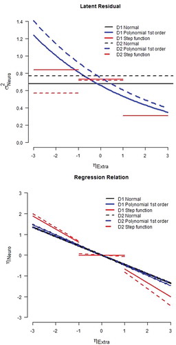
Comparing the AIC of the two models of choice (L-HETERO and S-FULL) showed that the S-FULL fitted the data best (discovery sample: AIC L_HETERO = 14657.03, AIC S_FULL = 14611.63; replication sample: AIC L_HETERO = 14522.87, AIC S_FULL = 14507.70). Comparing the parameter estimates of the two models (Table 8), the difference in the implied regression relation and residual variance are apparent. We plotted the regression relation and residual variance of the BASIC model, the L_HETERO, and the S_FULL model in Figure 4. Based on the parameters of L_HETERO model, the regression relation of the polynomial function is equal to the regression relation of the basic model. However, the residual variance is larger at the lower region of extroversion than in the higher region of extroversion (i.e., σ²[neuroticism | low extroversion] > σ² [neuroticism | high extroversion]). This implies a stronger relation between neuroticism and extroversion in the high regions of extroversion . For the S_FULL model, we note that the regression relation is only present at the lower and higher regions of extroversion (SD < –1 or SD > 1), whereas in the midrange (between –1 SD and +1 SD), there seems to be no relation between the two constructs. Additionally, we note that the residual variance is largest in the midrange, and smallest at the high tail of the distribution, which implies a stronger relation between neuroticism and extroversion in the high regions of extroversion.

TABLE 8 Parameter Estimates for the Two Data Sets Used in the Illustration of the Model

			Parameter estimates
			Non-linearity			Heteroskedasticity
Data	Function	Model	γ0	γ1		(log)ϕ0	(log)ϕ1
Data 1	Polynomial	BASIC	−.49(.03)	—		.68(.08)	—
		HETERO	−.49(.03)	—.05(.03)		.66(.08)	.81(.06)		*
		NON-L	–.48(.03)	–.02(.03)		.68(.08)	.82(.07)
		FULL	–.50(.03)			.66(.08)
			κ0	κ1	κ2	ξ0	ξ1	ξ2
	Step	BASIC	−.49(.03)	—	—	.68(.08)	—	—
		HETERO	−.52(.02)	—.40(.15)	—.25(.15)	.77(.07)	.08(.07)	−.41(.04)	*
		NON-L	–.21(.13)	–.62(.14)	–.66(.12)	.67(.05)	.11(.07)	–.42(.04)
		FULL	–.01(.12)			.73(.06)
			γ0	γ1		(log)ϕ0	(log)ϕ1
Data 2	Polynomial	BASIC	−.45(.03)	—	—	.77(.08)
		HETERO	−.45(.03)	—.08(.03)	—	.75(.08)	.81(.06)		*
		NON-L	–.43(.03)	–.03(.03)		.76(.08)	.84(.07)
		FULL	–.45(.03)			.76(.08)
			κ0	κ1	κ2	ξ0	ξ1	ξ2
	Step	BASIC	−.45(.03)			.77(.08)
		HETERO	−.52(.02)	−.38(.15)	−.15(.16)	.80(.00)	−.18(.08)	−.39(.00)	*
		NON-L	−.22(.12)	−.61(.15)	−.75(.13)	.76(.08)	−.15(.09)	−.41(.04)
		FULL	−.06(.12)			.72(.06)

FIGURE 4  Effect of the parameter estimates on the latent residual variance (top) and the regression relation (bottom). Parameter values of best fitting model are used, as given in Table 8.

DISCUSSION

In this article, we used the indirect mixture modeling approach to model latent heteroskedasticity and nonlinearity in latent regression using MML estimation. The approach is based on the MML estimation as presented by Bock and Aitkin (1981) in the context of IRT modeling, and by Klein and Moosbrugger (2000) in the context of structural equation modeling (see also Moosbrugger et al., 2009). Molenaar, Dolan, and de Boeck (2012; see also Molenaar, Dolan, & Verhelst, 2010) used this approach to model heteroskedasticity and nonlinearity in IRT and factor models.

The possibility to model nonlinearity and heteroskedasticity simultaneously is interesting for both statistical and theoretical reasons. As shown in the simulation study, ignoring heteroskedasticity in presence of nonlinearity leads to biased estimation of the nonlinearity in the regression relation. In the illustration, we showed the consequence of ignoring heteroskedasticity. Failing to model simultaneously heteroskedasticity and nonlinearity, we would have concluded that the relationship between extroversion and neuroticism was nonlinear, but we would not have been able to assess the effect of heteroskedasticity. As shown in the real data example, fitting the polynomial function would have led to a different conclusion.

We consider the flexibility in specifying the function to model nonlinearity and heteroskedasticity a useful feature of this approach. In the illustration, we demonstrated that using different functions to model the latent regression and latent residual provided greater insight into the underlying regression relation. Using the polynomial function, it appeared that the residual variance decreased with extroversion, and that the regression relation was constant over the range of extroversion. However, using the step function, we found that the residual variance was larger in the midrange of extroversion and smaller in the tails. Additionally, we showed that the regression relation was strong in the tails and absent in the midrange of extroversion. This observation underscores the importance of flexibility in the specification of the function with which heteroskedasticity and nonlinearity are modeled.

To establish the viability of the model, we investigated the performance of the model in a small-scale simulation study. We established that parameter recovery is accurate and that given reasonable sample sizes, power is acceptable. We observed lower power given opposite effects of nonlinearity and heteroskedasticity. This can be explained in terms of the detection of nonnormality in the data with regular tests such as the Shapiro–Wilks test. When the effects of nonlinearity and heteroskedasticity are in opposite directions, their effects on the distribution cancel out. The simulation study also showed that misspecification of the model does not lead to incorrect statistical inferences when estimating a parameter known to be zero. Given these results, we consider the model to be viable. However, we note that ignoring either heteroskedasticity or nonlinearity when both effects are known to be present in data does lead to biased estimation of the strength of the regression relation.

This study has the following limitations. First, we only considered a limited number of indicators of both the predictor and the dependent, although many psychological phenomena are measured with more indicators (e.g., items in the questionnaire). The addition of indicators is relatively straightforward. Second, we also considered a limited number of factors, although psychological theories often concern numerous constructs. Generalization of the model to multiple factors might be accomplished via the use of multivariate Gauss–Hermite quadratures. Within the MML framework, extension of the model might only be feasible for a small number of factors (up to five; see Wood et al., 2002). For larger models, a Bayesian estimation procedure is a viable option (e.g., Arminger & Muthén, 1998; Molenaar & Dolan, 2014). Third, we limited the simulation study to the first-order heteroskedasticity and first-order nonlinearity model. As discussed in Molenaar et al. (2010), and demonstrated in our example, the model can be extended to polynomial functions, other nonlinear functions, and step functions. As such, a variety of nonlinear relations can be considered and tested in practice. This method requires the specification of functions to accommodate nonlinearity and heteroskedasticity. For a more exploratory approach to nonlinearity of the regression function based on indirect mixture modeling, we refer to Bauer (2005; Pek et al., 2009), and for a recent exploratory data mining approach that can handle nonlinearity, we refer to Miller, Lubke, McArtor, and Bergeman (in press). Finally, we have assumed that the predictor and conditional dependent variable (i.e., conditional on the predictor) are normally distributed. Kelava et al. (2014) presented a nonlinear latent regression model with nonnormal predictors.

Notes

¹ The OpenMx script is available at www.dylanmolenaar.nl.

REFERENCES

- Arminger, G., & Muthén, B. (1998). A Bayesian approach to nonlinear latent variable models using the Gibbs sampler and the Metropolis–Hastings algorithm. Psychometrika, 63, 271–300. doi:10.1007/BF02294856
- Bauer, D. J. (2005). A semiparametric approach to modeling nonlinear relations among latent variables. Structural Equation Modeling, 12, 513–535. doi:10.1207/s15328007sem1204_1
- Bock, R. D., & Aitkin, M. (1981). Marginal maximum likelihood estimation of item parameters: Application of an EM algorithm. Psychometrika, 46, 443–459. doi:10.1007/BF02293801
- Boker, S., Neale, M., Maes, H., Wilde, M., Spiegel, M., Brick, T., … Fox, J. (2011). OpenMx: An open source extended structural equation modeling framework. Psychometrika, 76, 306–317. doi:10.1007/s11336-010-9200-6
- Bollen, K. A. (1995). Structural equation models that are nonlinear in latent variables: A least squares estimator. Sociological Methodology, 25, 223–251. doi:10.2307/271068
- Cacioppo, J. T., Hawkley, L. C., & Thisted, R. A. (2010). Perceived social isolation makes me sad: 5-year cross-lagged analyses of loneliness and depressive symptomatology in the Chicago health, aging, and social relations study. Psychology and Aging, 25, 453–463. doi:10.1037/a0017216
- Costa, P. T., Jr., & McCrae, R. R. (1985). The NEO personality inventory manual. Odessa, FL: Psychological Assessment Resources.
- Dolan, C. V., Schmittmann, V. D., Lubke, G. H., & Neale, M. C. (2005). Regime switching in the latent growth curve mixture model. Structural Equation Modeling, 12, 94–119. doi:10.1207/s15328007sem1201_5
- Dolan, C. V., & van der Maas, H. L. J. (1998). Fitting multivariate normal mixtures subject to structural equation modeling. Psychometrika, 63, 227–253. doi:10.1007/BF02294853
- Elshout, J. J., & Akkerman, A. E. (1975). Vijf persoonlijkheidsfaktoren test 5PFT: Handleiding [The Five Personality Factor Test (5PFT): Manual]. Nijmegen, The Netherlands: Berkhout B.V.
- Greene, W. H. (2011). Econometric analysis (7th ed.). Upper Saddle River, NJ: Prentice-Hall.
- Hooper, P. M. (1993). Iterative weighted least squares estimation in heteroscedastic linear models. Journal of the American Statistical Association, 88, 179–184.
- Huber, P. J. (1967). The behavior of maximum likelihood estimates under nonstandard conditions. In Proceedings of the Fifth Berkeley Symposium on Mathematical Statistics and Probability (vol. 1, pp. 221–233). University of California Press, Berkeley, CA.
- Jaccard, J., & Wan, C. K. (1996). LISREL analyses of interaction effects in multiple regression. Newbury Park, CA: Sage.
- Jöreskog, K. G., & Yang, F. (1996). Nonlinear structural equation models: The Kenny–Judd model with interaction effects. In G. A. Marcoulides & R. E. Schumacker (Eds.), Advanced structural equation modeling: Issues and techniques (pp. 57–87). Mahwah, NJ: Erlbaum.
- Kelava, A., Nagengast, B., & Brandt, H. (2014). A nonlinear structural equation mixture modeling approach for nonnormally distributed latent predictor variables. Structural Equation Modeling, 21, 468–481. doi:10.1080/10705511.2014.915379
- Kenny, D. A., & Judd, C. M. (1984). Estimating the nonlinear and interactive effects of latent variables. Psychological Bulletin, 96, 201–210. doi:10.1037/0033-2909.96.1.201
- Klein, A. G., & Moosbrugger, H. (2000). Maximum likelihood estimation of latent interaction effects with the LMS method. Psychometrika, 65, 457–474. doi:10.1007/BF02296338
- Klein, A. G., & Muthén, B. O. (2007). Quasi maximum likelihood estimation of structural equation models with multiple interaction and quadratic effects. Multivar Behavioral Researcher, 42, 647–674. doi:10.1080/00273170701710205
- Lubke, G. H., & Muthén, B. (2005). Investigating population heterogeneity with factor mixture models. Psychological Methods, 10, 21–39. doi:10.1037/1082-989X.10.1.21
- Marsh, H. W., Wen, Z., & Hau, K.-T. (2004). Structural equation models of latent interactions: Evaluation of alternative estimation strategies and indicator construction. Psychological Methods, 9, 275–300. doi:10.1037/1082-989X.9.3.275
- Miller, P. J., Lubke, G. H., McArtor, D. B., & Bergeman, C. S. (in press). Finding structure in data using multivariate tree boosting. Psychological Methods.
- Molenaar, D., & Dolan, C. V. (2014). Testing systematic genotype by environment interactions using item level data. Behavior Genetics, 44, 212–231. doi:10.1007/s10519-014-9647-9
- Molenaar, D., Dolan, C. V., & de Boeck, P. (2012). The heteroskedastic graded response model with a skewed latent trait: Testing statistical and substantive hypotheses related to skewed item category functions. Psychometrika, 77, 455–478. doi:10.1007/s11336-012-9273-5
- Molenaar, D., Dolan, C. V., & van der Maas, H. L. J. (2011). Modeling ability differentiation in the second-order factor model. Structural Equation Modeling, 18, 578–594. doi:10.1080/10705511.2011.607095
- Molenaar, D., Dolan, C. V., & Verhelst, N. (2010). Testing and modeling non-normality within the one factor model. British Journal of Mathematical and Statistical Psychology, 63, 293–317. doi:10.1348/000711009X456935
- Molenaar, D., Dolan, C. V., Wicherts, J. M., & van der Maas, H. L. J. (2010). Modeling differentiation of cognitive abilities within the higher-order factor model using moderated factor analysis. Intelligence, 38, 611–624. doi:10.1016/j.intell.2010.09.002
- Molenaar, D., van der Sluis, S., Boomsma, D. I., Haworth, C. M., Hewitt, J. K., Martin, N. G., … Dolan, C. V. (2013). Genotype by environment interactions in cognitive ability: A survey of 14 studies from four countries covering four age groups. Behavior Genetics, 43, 208–219. doi:10.1007/s10519-012-9581-7
- Moosbrugger, H., Schermelleh-Engel, K., Kelava, A., & Klein, A. G. (2009). Testing multiple nonlinear effects in structural equation modeling: A comparison of alternative estimation approaches. In T. Teo & M. S. Khine (Eds.), Structural equation modelling in educational research: Concepts and applications (pp. 103–136). Rotterdam, The Netherlands: Sense.
- Muthén, B., Khoo, S.-T., Francis, D. J., & Boscardin, C. K. (2003). Analysis of reading skills development from kindergarden through first grade: An application of growth mixture modeling to sequential processes. In S. P. Reise & N. Duan (Eds.), Multilevel modeling: Methodological advances, issues, and applications (pp. 71–89). Mahwah, NJ: Erlbaum.
- Pek, J., Sterba, S. K., Kok, B. E., & Bauer, D. J. (2009). Estimating and visualizing nonlinear relations among latent variables: A semiparametric approach. Multivariate Behavioral Research, 44, 407–436. doi:10.1080/00273170903103290
- Ping, J. R. A. (1996). Latent variable interaction and quadratic effect estimation: A two-step technique using structural equation analysis. Psychological Bulletin, 119, 166–175. doi:10.1037/0033-2909.119.1.166
- R Development Core Team. (2012). R: A language and environment for statistical computing. Vienna, Austria: R Foundation for Statistical Computing. Retrieved from http://www.R-project.org/
- Schmittmann, V. D., Dolan, C. V., van der Maas, H. L. J., & Neale, M. C. (2005). Discrete latent Markov models for normally distributed response data. Multivariate Behavioral Research, 40, 461–488. doi:10.1207/s15327906mbr4004_4
- Schumacker, R., & Marcoulides, G. (1998). Interaction and nonlinear effects in structural equation modeling. Mahwah, NJ: Erlbaum.
- Smits, I. A. M., Dolan, C. V., Vorst, H. C. M., Wicherts, J. M., & Timmerman, M. E. (2011). Cohort differences in big five personality factors over a period of 25 years. Journal of Personality and Social Psychology, 100, 1124–1138. doi:10.1037/a0022874
- Stroud, A. H., & Secrest, D. (1966). Gaussian quadrature formulas. Prentice-Hall: Englewood Cliffs, NJ.
- van der Sluis, S., Dolan, C. V., Neale, M. C., Boomsma, D. I., & Posthuma, D. (2006). Detecting genotype–environment interaction in MZ twin data: Comparing the Jinks & Fulker test and a new test based on marginal maximum likelihood estimation. Twin Research, 9, 377–392.
- Wall, M. M., Guo, J., & Amemiya, Y. (2012). Mixture factor analysis for approximating a nonnormally distributed continuous latent factor with continuous and dichotomous observed variables. Multivariate Behavioral Research, 47, 276–313. doi:10.1080/00273171.2012.658339
- White, H. (1980). A heteroskedasticity-consistent covariance matrix estimator and a direct test for heteroskedasticity. Econometrica, 48, 817–838. doi:10.2307/1912934
- Wood, R., Wilson, D. T., Gibbons, R. D., Schilling, S. G., Muraki, E., & Bock, R. D. (2002). TESTFACT:Test scoring, item statistics, and item factor analysis. Chicago, IL: Scientific Software International.