Drawing Conclusions from Cross-Lagged Relationships: Re-Considering the Role of the Time-Interval

Abstract

The cross-lagged panel model (CLPM), a discrete-time (DT) SEM model, is frequently used to gather evidence for (reciprocal) Granger-causal relationships when lacking an experimental design. However, it is well known that CLPMs can lead to different parameter estimates depending on the time-interval of observation. Consequently, this can lead to researchers drawing conflicting conclusions regarding the sign and/or dominance of relationships. Multiple authors have suggested the use of continuous-time models to address this issue.

In this article, we demonstrate the exact circumstances under which such conflicting conclusions occur. Specifically, we show that such conflicts are only avoided in general in the case of bivariate, stable, nonoscillating, first-order systems, when comparing models with uniform time-intervals between observations. In addition, we provide a range of tools, proofs, and guidelines regarding the comparison of discrete- and continuous-time parameter estimates.

Keywords:

• continuous-time SEM
• cross-lagged panel model (CLPM)
• first-order vector autoregressive (VAR(1)) model
• lagged effects

INTRODUCTION

The cross-lagged panel model (CLPM), a discrete-time (DT) structural equation modeling (SEM) model, is a popular method used to analyze longitudinal panel data consisting of multiple repeated measurements of a set of variables. The CLPM is conceptually similar to the first-order vector autoregressive (VAR(1)) model used in time series analysis (cf. Hamilton, 1994), which has seen a recent growth in popularity for the analysis of experience sampling data (cf. Bolger & Laurenceau, 2013; Chow, Ferrer, & Hsieh, 2011; Hamaker, Dolan, & Molenaar, 2005). This type of SEM model is particularly appealing in that it offers the opportunity to assess potentially Granger-causal (Granger, 1969) or predictive relationships between variables when lacking an experimental design, using cross-lagged regression parameters.

However, this type of lagged regression suffers from the well-known problem of time-interval dependency. That is, although this model takes into account the longitudinal structure of the data with respect to the order of measurement occasions, it does not explicitly account for the amount of time that elapses between measurement occasions. This has two major practical implications for researchers. First, if observations within a study are gathered with unequal time-intervals, the standard CLPM will lead to biased results, because it will model the unequal time-intervals as if they were equidistant. Second, even if all observations are equally-spaced in time, the estimated lagged effects will be specific to the time-interval used in the study. That is, the estimated lagged relationships between variables will vary as a function of the amount of time between measurements (a.o., Gollob & Reichardt, 1987). This means that researchers who study the same phenomenon with different uniform time-intervals will come across different estimates of seemingly the same lagged effects. Importantly, this can in some instances lead to researchers studying the same phenomena coming to opposite conclusions regarding the sign and relative strengths (i.e., order of predictive dominance) of lagged effects. To overcome both of the problems posed by the time-interval dependency issue, the use of a Continuous-Time (CT) Modeling approach has been suggested repeatedly in the literature (e.g., Boker, 2002; Chow et al., 2005; Oravecz, Tuerlinckx, & Vandekerckhove, 2009; Oud & Delsing, 2010a). In particular, both Voelkle, Oud, Davidov, and Schmidt (2012) and Boker, Neale, and Rausch (2004) have demonstrated how these models can be estimated in SEM-based software.

In the current article, we will focus specifically on the issue of comparability between CLPM effect estimates of the same phenomena when different uniform time-intervals are used in data collection. This is an issue that is particularly important in the social sciences at the moment, where issues such as replicability and meta-analyses have seen recent widespread critical attention. We offer an accessible account of the specific conditions under which conclusions regarding the sign and relative strengths of effects are invariant under different choices of uniform time-interval.

First, we will begin with an introduction to the key concepts behind the standard CLPM and its continuous-time equivalent, both SEM-based approaches, and a treatment of how these models are related to one another. This treatment includes a number of formulas and tools by which effect estimates based on another time-interval or time-scale, or using another model, can be made comparable, with corresponding R code in an Appendix. Second, we will examine the issue of researchers who use different uniform time-intervals to come to different conclusions with regard to the sign and relative strength of effects. Although previous authors have been at pains to point out that this can sometimes occur, we will elucidate the exact circumstances in which this will or will not occur. In the general case, within the first-order processes, only when researchers are studying univariate processes or stable bivariate processes with real eigenvalues, are such conclusions insensitive to the choice of uniform time-interval or choice of model. We conclude with some recommendations for substantive researchers and a discussion of related pertinent issues.

PRELIMINARIES

In this section, we will introduce the key concepts used throughout the rest of the article. The CLPM is briefly discussed, along with some shortfalls of this model which motivate the rest of the current article. Following this, we briefly introduce the continuous-time model (CTM) that has been suggested by various authors as a means of overcoming the two time-interval problems associated with the CLPM, a DT model. Finally, we will show how these two models can be related in a straightforward manner, a finding that is then utilized throughout the rest of the article.

The Discrete-Time (DT) Cross-Lagged Panel Model (CLPM)

The CLPM is a popular DT SEM-based model used for the analysis of longitudinal panel data, that is, data in which the same set of variables is measured repeatedly at several measurement occasions (cf. Finkel, 1995; Hamaker, Kuiper, & Grasman, 2015; Rogosa, 1980). The CLPM can be seen as an extension to panel data of the first-order vector autoregressive (VAR(1)) model from time-series analysis (cf. Hamilton, 1994). For the sake of simplicity, although we will discuss issues relevant to general VAR(1) models, we will use the CLPM term throughout. In these models, q variables (y) measured at each measurement occasion (m) are regressed on themselves and each other at the previous measurement occasion ($m-1$). For the sake of notational simplicity, and without loss of generality, we will assume throughout that the variables y are standardized, and thus, so too are all parameter estimates. Notably, when comparing parameter estimates, one should examine the standardized parameters to allow for a fair comparison of the size of lagged effect parameters.

The CLPM can then be represented in the general case, using solely the structural equation, as:

(1) ${\mathit{y}}_m=\mathbf{\Phi }{\mathit{y}}_{m-1}+{ϵ}_m$(1)

where ${\mathit{y}}_m$ are the q standardized variables of interest at measurement occasion m, which implies an intercept of zero and results in standardized parameters; ${ϵ}_m$ represents a m -vector of errors that are independent and identically distributed but may be contemporaneously correlated; and Φ is the $q\times q$ matrix consisting of standardized autoregressive and cross-lagged parameters. The elements of the effect matrix Φ are denoted by ${\varphi }_{jk}$ and represent the effect of variable j at measurement occasion $m-1$ on variable k at measurement occasion m for $j,k=1,\dots ,q$, which is the same for all measurement occasions (m). In case of a stable and therefore stationary process, the modulus (i.e., the absolute value) of the eigenvalues are smaller than 1. This implies that the process is mean-reverting, that is, tends to drift toward its long-term mean, here, zero, because of the standardized variables.

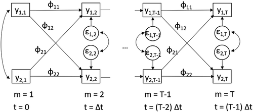
An example of a bivariate CLPM is shown in Figure 1. Researchers who apply the CLPM are generally interested in the standardized cross-lagged parameters, ${\varphi }_{12}$ and ${\varphi }_{21}$ in Figure 1, and the comparison of their relative strengths. Stability of the constructs is controlled for through the inclusion of the autoregressive effects, that is, parameters ${\varphi }_{11}$ and ${\varphi }_{22}$ in Figure 1 (cf. Rogosa, 1980). Due to the fact that the CLPM controls for this stability, it is often believed that the cross-lagged regression parameters obtained with this model are the most appropriate measures for studying causality in longitudinal correlational data (Deary, Allerhand, & Der, 2009) and determining which variable has a stronger causal influence on the other (Bentler & Speckart, 1981). Such conclusions are based on the notion of Granger causality (Granger, 1969).¹ The CLPM is a flexible model that can be used for many different numbers of variables. Adaptations of the CLPM have been proposed, for example, for the study of mediation (Maxwell, Cole, & Mitchell, 2011) and the estimation of dynamical networks (Bringmann et al., 2013).

FIGURE 1 Bivariate relationship between $y_1$ (e.g., child health) and $y_2$ (e.g., maternal health) for time points $t=0,\dots ,(T-1)\mathrm{\Delta }t$ with autoregression parameters ${\varphi }_{11}$ and ${\varphi }_{22}$, and cross-lagged parameters ${\varphi }_{12}$ and ${\varphi }_{21}$. In case of a symmetric relationship, the cross-lagged/reciprocal parameters are equal, that is, ${\varphi }_{12}={\varphi }_{21}$.

The CLPM can be described as a DT model in that the model does not explicitly account for the length of the time-intervals between measurement occasions. Thus, the CLPM fails to account for the fact that: (i) the time-intervals between measurement occasions may be unequal, and (ii) the variables measured continue to exist and influence each other in-between measurement occasions. Although this may appear to be mainly theoretical or conceptual concerns, the DT nature of the CLPM has rather practical implications for researchers. As has been pointed out by numerous researchers (e.g., Gollob & Reichardt, 1987; Pelz & Lew, 1970; Voelkle & Oud, 2013), the estimated cross-lagged and autoregressive effect matrix Φ may vary as a function of the length of the time-interval, that is, the amount of time that elapses, between two consecutive measurement occasions: $\mathrm{\Delta }{t}_m=t_m-t_{m-1}$, where $t_m$ represents the exact time point at which measurement m is made. This means that two researchers studying the same phenomenon may come across completely different estimates of the same effects purely due to differences in the choice of which time-interval to use, even when they both have equal time-intervals between measurements within their studies.

To reflect the time-interval dependency of the CLPM, we can rewrite the DT effect matrix Φ as $\mathbf{\Phi }(\mathrm{\Delta }{t}_m)$. Notably, in the case of unequal time-intervals, the estimated Φ matrix is a mix of $\mathbf{\Phi }(\mathrm{\Delta }{t}_m)$ estimates for different time-intervals and thus most probably a biased estimate. Therefore, in this article, we will focus on applications of the CLPM in cases where there is a uniform time-interval of measurement, that is, $\mathrm{\Delta }{t}_m=\mathrm{\Delta }t$ for all m. Consequently, we will use $\mathbf{\Phi }(\mathrm{\Delta }t)$ throughout the article.

Continuous-Time Model (CTM) Equivalent of the CLPM

CTM overcomes the time-interval dependency problem by explicitly taking the time-interval dependent nature of the relationships between variables at different measurement occasions into account. Conceptually, the CTM assumes that the processes of interest take on values and, moreover, influence each other at every moment in time, not only on the occasions at which the researcher measures them. For a substantive rationale for using this type of model in a psychology or social science setting, we refer readers to Boker (2002).

The CTM of interest in this case is the first-order stochastic differential equation model also referred to as the multivariate Ornstein-Uhlenbeck process, that is,

(2) $\frac{dy(t)}{dt}=\mathit{A}y(t)+\mathrm{\Omega }\frac{d\mathit{w}(t)}{dt}$(2)

where the $q\times q$ matrix A, referred to as the drift matrix, contains the standardized parameters which relate the values of the standardized variables in y at a particular time t to the derivative (i.e., rate of change) in $\mathit{y}(t)$ with respect to time (Oravecz, Tuerlinckx, & Vandekerckhove, 2011; Oud & Delsing, 2010b; Voelkle & Oud, 2013). The elements of A are denoted ${\alpha }_{jk}$, representing the standardized effect of variable j on the rate of change in variable k for $j,k=1,\dots ,q$. In case of a stable and therefore stationary process, the eigenvalues of A are negative. The last term on the right-hand side of Equation 2 is the continuous-time version of a random error process that is independent and identically distributed, but may be contemporaneously correlated. For a detailed discussion, see among others Oud and Delsing (2010b) and, for details on how this model can be estimated in a SEM-framework, see e.g., Boker (2002); Oud and Delsing (2010b).

This CTM can be considered the continuous-time analoge of a DT VAR(1) process, that is, the CLPM shown in Equation 1. However, the differential equation at the heart of the CTM approach represents quite a different approach to modeling longitudinal processes than the CLPM. The effect matrix A at the core of the model, shown in Equation 2, does not represent the relationships between variables at different measurement occasions, but rather the relationship between the values of the variables y at time t and their instantaneous rate of change. In other words, the drift matrix represents how we would expect the values of the variables y to change over a very short time-interval after time t, given the values of those variables at time t. The drift matrix controls the strength and the direction of the centralizing tendency or dampening force (Oravecz & Tuerlinckx, 2011; Oravecz et al., 2009): the tendency to stay near the average position of the process (i.e., µ), which is zero in case of standardized variables. For more details regarding the interpretation of the drift matrix, see Ryan, Kuiper, and Hamaker (in press).

Relating the CTM and the Discrete-Time Model (CLPM)

Although the DT CLPM and the CTM discussed above represent distinct ways of modeling longitudinal processes, they are related to each other. It can be shown that the DT effect matrix $\mathbf{\Phi }(\mathrm{\Delta }t)$ is actually a function of the drift matrix A:

(3) $\mathbf{\Phi }(\mathrm{\Delta }t)=e^{\mathit{A}\mathrm{\Delta }t}$(3)

where $\mathbf{\Phi }(\mathrm{\Delta }t)$, A and $\mathrm{\Delta }t$ are as defined above, and e is the matrix exponential (if $q>1$). Equality 3 will be key to the ideas and tools presented in this article, as well as the proofs supporting them. For an accessible introduction to the matrix exponential and the logic behind this equality, see Voelkle et al. (2012).

Note that all CTMs have a unique DT-model equivalent; however, not all DT models have a unique CTM equivalent. Furthermore, when the DT process is not smooth and differentiable (Boker & Nesselroade, 2002), there is no CTM equivalent at all. An example is a univariate, first-order, autoregressive process with a negative autoregressive parameter, because an exponential is always positive.² As such, we will refer to DT models with a CTM equivalent as ones that exhibit ‘positive autoregression’. Note that such ‘positive autoregression’, first-order processes are often plausible when analyzing psychological processes (cf. Koval & Kuppens, 2012; Oravecz & Tuerlinckx, 2011). In some cases, there may be many CTMs which generate the same DT-model effect matrix $\mathbf{\Phi }(\mathrm{\Delta }t)$. This occurs when $\mathbf{\Phi }(\mathrm{\Delta }t)$ has complex eigenvalues, meaning there are multiple periodic-equivalent or aliasing drift matrices A (cf. Hamerle, Nagl, & Singer, 1991; Yue, Thunberg, & Goncalves, 2016). In practice, this means that we cannot solve uniquely for A given $\mathbf{\Phi }(\mathrm{\Delta }t)$ with complex eigenvalues. Notably, the converse is possible, that is, one can solve uniquely for $\mathbf{\Phi }(\mathrm{\Delta }t)$ given an A with complex eigenvalues.

We present here some properties of the exponential relationship which will be used in the proofs found in later sections of the article. We make use of an eigenvalue decomposition of the effect matrix A, that is,

(4) $\mathit{A}=V{D}_A{V}^{-1}$(4)

where V is a matrix of eigenvectors and ${\mathit{D}}_A$ is a diagonal matrix containing the eigenvalues of A. For more details on this, see Appendix A. The decomposition in (4) is important as it allows us to more explicitly define how we can solve for A and $\mathbf{\Phi }(\mathrm{\Delta }t)$ given one or the other, as will be discussed next, which is helpful in comparing effect estimates. Appendix B gives the accompanying proofs, as well as details on how to calculate the expressions in the statistical programming language R (R Core Team, 2013).

To find $\mathbf{\Phi }(\mathrm{\Delta }t)$ given A we can use,

(5) $\mathbf{\Phi }(\mathrm{\Delta }t)=e^{\mathit{A}\mathrm{\Delta }t}=\mathit{V}{e}^{{\mathit{D}}_A\mathrm{\Delta }t}{\mathit{V}}^{-1}$(5)

where $e^{{\mathit{D}}_{\mathit{A}}\mathrm{\Delta }t}(={\mathit{D}}_{\mathbf{\Phi }(\mathrm{\Delta }t)})$ represents the diagonal matrix containing the scalar exponentials of the eigenvalues of A multiplied by the scalar $\mathrm{\Delta }t$. We can use this to relate any two $\mathbf{\Phi }(\mathrm{\Delta }t)$ matrices which use different uniform time-intervals, say, $\mathbf{\Phi }(d_1)$ and $\mathbf{\Phi }(d_2)$, with the equality,

(6) $\mathbf{\Phi }(d_2)=(\mathbf{\Phi }(d_1){)}^{\frac{d_2}{d_1}}.$(6)

Furthermore, we can solve for $\mathit{A}$ given any $\mathbf{\Phi }(\mathrm{\Delta }t)$ by using,

(7) $\mathit{A}=\mathit{V}(log({\mathit{D}}_{\mathbf{\Phi }(\mathit{D}t)})/\mathrm{\Delta }t){\mathit{V}}^{-1},$(7)

where ${\mathit{D}}_{\mathbf{\Phi }(\mathit{D}t)}$ is the diagonal matrix containing the eigenvalues of $\mathbf{\Phi }(\mathrm{\Delta }t)$. It is important to note that this expression should only be used when $\mathbf{\Phi }(\mathrm{\Delta }t)$ does not have complex eigenvalues.

With regard to the comparison of drift matrices A between researchers, different estimates can result from the same process or even the same data if researchers choose a different time-scale. That is, the estimate of A depends on the unit of time we choose for $\mathrm{\Delta }t$ (e.g., half-hours vs. hours or weeks vs. months). However, assuming each researcher is capturing the same underlying dynamics, no contradictory conclusions will result: see Appendix B for more details, including a useful transformation to use in case of different time-scales.

COMPARING RESULTS BASED ON DIFFERENT UNIFORM TIME-INTERVALS

Until now we have seen that the parameter estimates of the CLPM vary as a function of the time-interval between measurements, and introduced the alternative CTM that explains this phenomenon. We now wish to establish in what circumstances this time-interval dependency leads to misleading or inconsistent substantive conclusions. We first distinguish three types of substantive conclusions researchers may be interested in. Subsequently, we examine whether inconsistencies in these conclusions occur due to the use of different uniform time-intervals, in the context of bivariate and higher-variate CLPMs.

Three Types of Substantive Conclusions in Terms of Standardized Model Parameters

Here, we define three main types of conclusions which researchers are generally interested in, and which are based on the relative size or sign (positive vs. negative) of parameters of the CLPM. For each of these types, we end with an example of a misleading result in terms of matrix elements $(p,s)$ (i.e., ${\varphi }_{ps}(\mathrm{\Delta }t)$) which can occur using two different uniform time-intervals, namely for $\mathrm{\Delta }t=d_1$ and $d_2$ (both finite and positive). Notably, we express these inequalities in terms of the population parameters, and not estimates. The reason for this is that we wish to make clear that these are misleading conclusions which may occur even in scenarios in which the parameter estimates are highly precise.

I. Order of dominance of the standardized autoregression effects.

Although researchers are generally more interested in the cross-lagged effects, they may also be interested in determining which of the processes under investigation is most stable by comparing the size of the corresponding standardized autoregressive effects. For instance, Koval and Kuppens (2012) study the autoregressive relationship of emotional inertia, and individual differences therein.

A misleading result is obtained if, for example,

$\begin{array}{cccc}{\varphi }_{pp}(d_1)>{\varphi }_{ss}(d_1)& & & {\varphi }_{pp}(d_2)<{\varphi }_{ss}(d_2),\mathrm{f}\mathrm{o}\mathrm{r}p\ne s.\end{array}$

II. Order of dominance of the cross-lagged effects.

Researchers are generally interested in whether the standardized cross-lagged effect of $y_1$ on $y_2$ is greater than the standardized cross-lagged effect of $y_2$ on $y_1$, or vice versa. For instance, Nohe, Meier, Sonntag, and Michel (2015) conduct a meta-analysis in which they compare the lagged effect of work-family conflict on strain to the lagged effect of strain on work-family conflict. As another example, in a sample of persons diagnosed with burnout, Schuurman, Ferrer, De Boer-Sonnenschein, and Hamaker (2016) investigated whether the effect of competence at occasion $m-1$ on exhaustion at occasion m was stronger or weaker than the corresponding cross-lagged effect of exhaustion on competence.

A misleading result is obtained if, for example, for ‘corresponding’ cross-lagged effects,

$(\mathrm{a}){\varphi }_{ps}(d_1)>{\varphi }_{sp}(d_1)\mathrm{\&}{\varphi }_{ps}(d_2)<{\varphi }_{sp}(d_2),\mathrm{f}\mathrm{o}\mathrm{r}p\ne s$

In the general multivariate case, we may also be interested in comparing any cross-lagged parameters we estimate. In this case, a misleading result is obtained if:

$(\mathrm{b}){\varphi }_{ps}(d_1)>{\varphi }_{uv}(d_1)\mathrm{\&}{\varphi }_{ps}(d_2)<{\varphi }_{uv}(d_2),\mathrm{f}\mathrm{o}\mathrm{r}p\ne s\mathrm{a}\mathrm{n}\mathrm{d}u\ne v$

III. Sign of the standardized cross-lagged effect.

Researchers are also generally interested in whether, for example, the cross-lagged effect of $y_{1,m-1}$ (e.g., physical well-being) on $y_{2,m}$ (e.g., social well-being) is positive or negative. For example, Schuurman et al. (2016) inspect and interpret the sign of the cross-lagged effects before comparing the ordering.

A misleading result is obtained if, for example,

${\varphi }_{ps}(d_1)>0\mathrm{\&}{\varphi }_{ps}(d_2)<0,\mathrm{f}\mathrm{o}\mathrm{r}p\ne s.$

These are three types of conclusions, regarding the ordering and sign of the lagged effects, which are commonly of interest to substantive researchers. The interested reader is referred to the Misleading Results section where we, among others, discuss other possible substantive conclusions researchers might wish to make.

No Misleading Conclusions: Bivariate, Stable, Nonoscillating, First-Order Systems

We first inspect the case of bivariate CLPMs, that is, bivariate first-order systems, see Figure 1 for an example. Let us assume, without loss of generalization, the following values for the $2\times 2$ eigenvector-matrix V and the $2\times 2$ eigenvalue-diagonal-matrix ${\mathit{D}}_{\mathbf{\Phi }(d_{\mathbf{1}})}$ of $\mathbf{\Phi }(\mathrm{\Delta }t=d_1)$:

$\mathit{V}=\left(\begin{array}{cc}{v}_{11}& v_{12}\\ v_{21}& v_{22}\end{array}\right)$

${\mathit{D}}_{\mathbf{\Phi }(d_{\mathbf{1}})}=\left(\begin{array}{cc}{\lambda }_1& 0\\ 0& {\lambda }_2\end{array}\right),$

with ${\lambda }_1$ and ${\lambda }_2$ the eigenvalues of $\mathbf{\Phi }(\mathrm{\Delta }t=d_1)$.³ Consequently, ${\mathit{V}}^{-1}$ is given by:

${\mathit{V}}^{-1}=\frac{1}{|\mathit{V}|}\left(\begin{array}{cc}{v}_{22}& -v_{12}\\ -v_{21}& v_{11}\end{array}\right),\mathrm{w}\mathrm{h}\mathrm{e}\mathrm{r}\mathrm{e}|\mathit{V}|=v_{11}\cdot v_{22}-v_{12}\cdot v_{21},$

and $\mathbf{\Phi }(d_1)$ by

$\mathbf{\Phi }(d_1)=\frac{1}{\left|V\right|}\left(\begin{array}{cc}{v}_{11}\cdot {\lambda }_1\cdot v_{22}-v_{12}\cdot v_{21}\cdot {\lambda }_2& -({\lambda }_1-{\lambda }_2)\cdot v_{11}\cdot v_{12}\\ ({\lambda }_1-{\lambda }_2)\cdot v_{21}\cdot v_{22}& -v_{12}\cdot v_{21}\cdot {\lambda }_1+v_{11}\cdot v_{22}\cdot {\lambda }_2\end{array}\right).$

From Equation 6, using $n=d_2/d_1$ for ease of notation, it follows that:

$\begin{array}{rl}& \mathbf{\Phi }(d_2)=(\mathbf{\Phi }(d_1){)}^n\\ & =V(D_{\mathbf{\Phi }(d_{\mathbf{1}})}{)}^n{V}^{-1}\end{array}$

$=\frac{1}{\left|\mathit{V}\right|}\left(\begin{array}{cc}{v}_{11}\cdot {\lambda }_1^n\cdot v_{22}-v_{12}\cdot v_{21}\cdot {\lambda }_2^n& -({\lambda }_1^n-{\lambda }_2^n)\cdot v_{11}\cdot v_{12}\\ ({\lambda }_1^n-{\lambda }_2^n)\cdot v_{21}\cdot v_{22}& -v_{12}\cdot v_{21}\cdot {\lambda }_1^n+v_{11}\cdot v_{22}\cdot {\lambda }_2^n\end{array}\right),$

with

$({\mathit{D}}_{\mathbf{\Phi }(d_{\mathbf{1}})}{)}^n=\left(\begin{array}{cc}{\lambda }_1^n& 0\\ 0& {\lambda }_2^n\end{array}\right).$

We can assess whether it is possible for misleading conclusions I to III to occur in the bivariate case by expressing the associated parameter inequalities in terms of eigenvalues and eigenvectors. Namely, all three types of misleading results are obtained when the sign of $({\lambda }_1-{\lambda }_2)$ differs from that of $({\lambda }_1^n-{\lambda }_2^n)$.

Thus, to assess whether these types of misleading conclusions can occur in bivariate, first-order systems based on the use of a different uniform time-interval, it suffices to assess whether there exists an ${\lambda }_1$, ${\lambda }_2$ and $n$ such that ${\lambda }_1>{\lambda }_2$ and ${\lambda }_1^n<{\lambda }_2^n$ or vice versa. For a stable, ‘positive autoregression’, first-order process with real eigenvalues, the eigenvalues ${\lambda }_1$ and ${\lambda }_2$ of $\mathbf{\Phi }(d_1)$ lie between 0 and 1. In that case, there exist no $n$ such that the sign of $({\lambda }_1-{\lambda }_2)$ differs from that of $({\lambda }_1^n-{\lambda }_2^n)$. Therefore, misleading conclusions I to III cannot occur when inspecting bivariate, stable, ‘positive autoregression’, nonoscillating, first-order systems employing different uniform time-intervals. Notably, the conclusions one would draw from the continuous-time effect matrix A in a bivariate, stable, nonoscillating, first-order setting are the same as those one would draw from DT model at any uniform time-interval, which is shown in Appendix C.

In sum, researchers will not come to misleading or inconsistent conclusions I to III in the case of bivariate, stable, first-order systems with real eigenvalues due to the use of a different uniform time-interval; that is, it is not possible to: (i) obtain a different sign in cross-lagged effects; (ii) find a different dominant cross-lagged effect; or (iii) find a different dominant autoregression effect. We will illustrate this next with an example.

Example

We will use the artificial example of Voelkle et al. (2012): Suppose, we are examining two variables ($q=2$), child’s health and maternal health. We are interested in the effect of child’s health ($y_{1,m-1}$) on maternal health one time period later ($y_{2,m}$), as well as the effect maternal health ($y_{2,m-1}$) has on child health one time period later ($y_{1,m}$), that is, ${\varphi }_{12}$ and ${\varphi }_{21}$ in Figure 1. Assume that the underlying drift matrix is given as:

$\mathit{A}=\left(\begin{array}{cc}-0.4472& 0.2320\\ 0.0435& -0.1170\end{array}\right).$

Now, take that we collect data generated by this underlying continuous-time process at time-intervals of $\mathrm{\Delta }t=1$ (e.g., months). Estimating the DT standardized effect matrix (asymptotically) yields:

$\mathbf{\Phi }(\mathrm{\Delta }t=1)=\left(\begin{array}{cc}0.64& 0.18\\ 0.03& 0.89\end{array}\right).$

Examining this effect matrix, we could make the following three conclusions: (i) maternal health is more stable, that is, has a stronger standardized autoregressive effect, than child’s health, that is, ${\varphi }_{22}=0.89>{\varphi }_{11}=0.64$; (ii) the standardized effect of maternal health on child’s health is greater than the effect of child’s health on maternal health, that is, ${\varphi }_{12}=0.18>{\varphi }_{21}=0.03$; (iii) both standardized cross-lagged effects are positive, that is, ${\varphi }_{12}=0.18>0$ & ${\varphi }_{21}=0.03>0$.

Now, suppose that we had chosen a time-interval for data collection that was twice as long, that is, $\mathrm{\Delta }t=2$ (e.g., bi-monthly). In that case, we would have (asymptotically) come to the following DT standardized effect matrix:

$\mathbf{\Phi }(\mathrm{\Delta }t=2)=\left(\begin{array}{cc}0.42& 0.27\\ 0.05& 0.80\end{array}\right).$

We can see that, although the standardized estimates for each cross-lagged and autoregressive effects change with this new time-interval, the conclusions drawn from this effect matrix are same as for those drawn from the matrix with the shorter time-interval: (i) ${\varphi }_{22}=0.80>{\varphi }_{11}=0.42$; (ii) ${\varphi }_{12}=0.27>{\varphi }_{21}=0.05$; and (iii) ${\varphi }_{12}=0.27>0$ & ${\varphi }_{21}=0.05>0$.

Using Equation 5, we can derive the DT standardized effect matrix for any time-interval. This can be plotted, as done in Figure 2, and is referred to as $\mathbf{\Phi }(\mathrm{\Delta }t)$ plot in this article. The $\mathbf{\Phi }(\mathrm{\Delta }t)$ in Figure 2 shows that, for all time-intervals, one will not find misleading conclusions: (i) & (ii) the autoregressive and cross-lagged effects do not cross each other, which implies no difference in order of dominance; and (iii) the cross-lagged effects do not cross the zero-line at any time-interval, which implies the same sign over the whole time range.

FIGURE 2 $\mathbf{\Phi }(\mathrm{\Delta }t)$plot: A bivariate example of how the parameter values (i.e., the elements in $\mathbf{\Phi }(\mathrm{\Delta }t)$) change as a function of the time-interval $\mathrm{\Delta }t$.

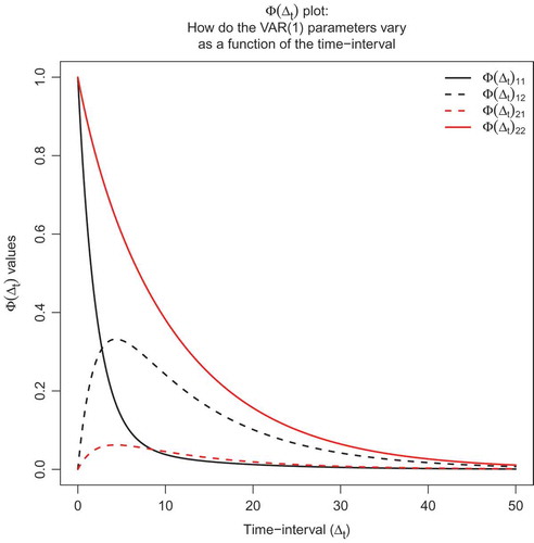
Furthermore, we can see that we reach the same conclusions when examining only the drift matrix A: (i) maternal health ($y_2$) is more stable, that is, has an autoregressive effect closer to zero, than child’s health, that is, $\left|{\alpha }_{22}\left|=\right|-0.1170\right|<\left|{\alpha }_{11}\left|=\right|-0.4472\right|$; because the diagonal elements will often be negative, we can also state: ${\alpha }_{22}=-0.1170>{\alpha }_{11}=-0.4472$; (ii) the effect of maternal health on child’s health are greater than the effect of child’s health on maternal health, that is, ${\alpha }_{12}=0.2320>{\alpha }_{21}=0.0435$; (iii) both cross-lagged effects are positive, that is, ${\alpha }_{12}=0.2320>0$ & ${\alpha }_{21}=0.0435>0$.

In the next subsection, we will discuss that equivalence of conclusions I to II drawn in the context of different uniform time-intervals of measurement does not hold in general when we are dealing with other types of bivariate systems or systems of more than two variables.

Misleading Conclusions

Although the substantive conclusions I to III are robust for using different uniform time-intervals in DT, first-order models that are bivariate, stable, and nonoscillating, this serves as the exception that proves the rule. To the best of our knowledge, the only equivalence that does exist in general is in the case of symmetric effects matrices, implying equal ‘corresponding’ cross-lagged effects, which is shown in Appendix D. Namely, if one finds a symmetric relationship, this will also be symmetric with every other choice of time-interval and model. Consequently, ${\varphi }_{ps}={\varphi }_{sp}$ (and also ${\alpha }_{ps}={\alpha }_{sp}$) for all $s,p=1,\dots ,q$ and thus misleading conclusion IIa will not occur. Nevertheless, misleading conclusions I, IIb, and III are still possible when modeling a system of more than two variables. Moreover, in case of a nonsymmetric effects matrix, even all substantive conclusions can be misleading, that is, I, IIa, IIb, and III. Multiple examples of misleading results in trivariate, first-order systems can be found in, for instance, Oud (2002, pp. 13–15) and Reichardt (2011).

In sum, except for DT, first-order models that are bivariate, stable, and nonoscillating misleading results can arise, also for the other bivariate, first-order systems. The remaining systems can be classified as follows:

• bi- and higher-variate, first-order systems with complex eigenvalues (both stable and unstable);

• bi- and higher-variate, unstable, first-order systems with real eigenvalues;

• tri- and higher-variate, stable, first-order systems with real eigenvalues.

Next, we will illustrate that misleading results can arise in the above classes of systems, by giving a (counter-)example. Additionally, we will illustrate that misleading results can arise when inspecting other types of conclusions, already in case of bivariate, stable, nonoscillating, first-order systems.

Bivariate, first-order systems with complex eigenvalues counter-example

In case of bivariate, first-order systems with complex eigenvalues, researchers can draw misleading conclusions I to III from $\mathbf{\Phi }(\mathrm{\Delta }t)$ depending on the time-interval chosen. In Appendix E we show that it is possible to specify ranges of $\mathrm{\Delta }t$ for which the sign and order of dominance (of autoregressive and of cross-lagged parameters) are invariant. Furthermore, we show that for every other range the substantive conclusions I to III made from $\mathbf{\Phi }(\mathrm{\Delta }t)$ match those made from the drift matrix. Figure 3 displays the $\mathbf{\Phi }(\mathrm{\Delta }t)$ plot for a system with

$\mathit{A}=\left(\begin{array}{cc}-1.79& 0.79\\ -3.93& -0.21\end{array}\right).$

FIGURE 3 The $\mathbf{\Phi }(\mathrm{\Delta }t)$ plot for a bivariate $\mathbf{\Phi }(\mathrm{\Delta }t)$ with complex eigenvalues, where conclusions I to III may differ per time-interval $\mathrm{\Delta }t$.

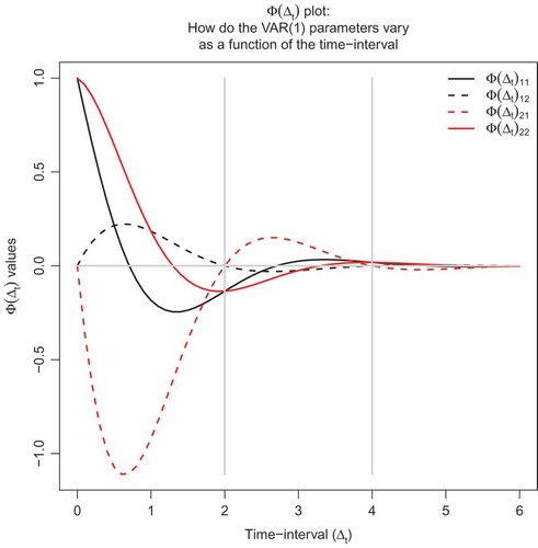
This drift matrix reflects an oscillating system with eigenvalues $-1\pm \iota 0.5\pi$ and eigenvectors $(1,1\pm \iota 2)$. From the $\mathbf{\Phi }(\mathrm{\Delta }t)$ plot, one can see that for $\mathrm{\Delta }t$ between 0 and 2 and between 4 and 6: (i) ${\varphi }_{11}<{\varphi }_{22}$; (ii) $\left|{\varphi }_{12}\right|<\left|{\varphi }_{21}\right|$; and (iii) ${\varphi }_{12}>0$ & ${\varphi }_{21}<0$. Thus, for time-intervals $\mathrm{\Delta }t$ between 0 and 2 and between 4 and 6, substantive conclusions I to III are not misleading. From the $\mathbf{\Phi }(\mathrm{\Delta }t)$ plot, one can also see that for $\mathrm{\Delta }t$ between 2 and 4: (i) ${\varphi }_{11}<{\varphi }_{22}$; (ii) $\left|{\varphi }_{12}\right|>\left|{\varphi }_{21}\right|$; and (iii) ${\varphi }_{12}<0$ & ${\varphi }_{21}<0$. Thus, for time-intervals $\mathrm{\Delta }t$ between 2 and 4, substantive conclusions I to III are not misleading. Note that the results for these ranges differ. Hence, for some combinations of $\mathrm{\Delta }t$ values, one will obtain misleading conclusions I to III. Additionally, from the drift matrix, one concludes that: (i) $\left|{\alpha }_{11}\left|=1.79>\right|{\alpha }_{22}|=0.21\right.$; because the diagonal elements are negative, we can also state: ${\alpha }_{11}=-1.79<{\alpha }_{22}=-0.21$; (ii) $\left|{\alpha }_{12}\right|=0.79<{\alpha }_{21}=3.93$; (iii) ${\alpha }_{12}=0.79>0$ & ${\alpha }_{21}=-3.93<0$. Thus, for time-intervals $\mathrm{\Delta }t$ between 0 and 2 and between 4 and 6, substantive conclusions I to III are not misleading when comparing it to the ones based on A. However, for time-intervals $\mathrm{\Delta }t$ between 2 and 4, conclusions I to III are misleading when comparing it to the ones based on A. Be aware that, when we are dealing with processes with complex eigenvalues, one needs to estimate the CTM directly, rather than apply the transformation in Equation 13. That is to say, given the nonunique solutions when solving for A from a $\mathbf{\Phi }(\mathrm{\Delta }t)$ with complex eigenvalues (e.g., using Equation 13), even the various possible (i.e., aliasing) drift matrices may lead to different conclusions regarding the signs and orderings of dominance. This can, for example, be seen from the aliasing drift matrices found in Hamerle et al. (1991, pp. 203, 209).

In sum, in case of bi- or higher-variate systems with complex eigenvalues, conclusions I to III based on DT-model effect estimates may be contradictory depending on the time-interval of observation.

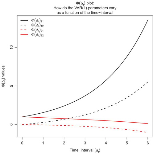
Bivariate, unstable, first-order systems with real eigenvalues counter-example

When the bi- or higher-variate, first-order process with real eigenvalues is not stable, conclusions I to III can be contradictory across different time-intervals. A first-order process is unstable if at least one eigenvalue has a positive real part. In Figure 4 the $\mathbf{\Phi }(\mathrm{\Delta }t)$ plot is depicted for a bivariate, first-order process with one positive and one negative eigenvalue. Here, we see that the ordering of effects changes for $\mathrm{\Delta }t>2$.

FIGURE 4 The $\mathbf{\Phi }(\mathrm{\Delta }t)$ plot for a unstable, bivariate $\mathbf{\Phi }(\mathrm{\Delta }t)$ with one negative and one positive real eigenvalue, where conclusions I to III may differ per time-interval $\mathrm{\Delta }t$.

Trivariate, stable, first-order systems with real eigenvalues counter-example

Let us consider the following $3\times 3$ drift matrix:

$\mathit{A}=\left(\begin{array}{ccc}-0.39& 0.01& 0.00\\ 0.32& -0.35& -0.04\\ -1.46& 1.18& -0.83\end{array}\right),$

where all three eigenvalues are real and negative: −0.67, −0.55, and −0.35, thus reflecting a stable and therefore stationary process with real eigenvalues. In Figure 5, one can see how the elements in $\mathbf{\Phi }(\mathrm{\Delta }t)$ change as a function of $\mathrm{\Delta }t$. When inspecting the autoregressive effects, one can see that the ordering for ${\varphi }_{11}$ and ${\varphi }_{22}$ changes as a function of the time-interval $\mathrm{\Delta }t$, that is, for small time-intervals, ${\varphi }_{11}$ is lower and, for longer time-intervals (approximately $\mathrm{\Delta }t>2.5$), it is higher than ${\varphi }_{22}$. Hence, we see misleading conclusion I.

FIGURE 5 The $\mathbf{\Phi }(\mathrm{\Delta }t)$ plot for a trivariate $\mathbf{\Phi }(\mathrm{\Delta }t)$, with change in dominance and sign, that is, where conclusions I to III may differ per time-interval $\mathrm{\Delta }t$.

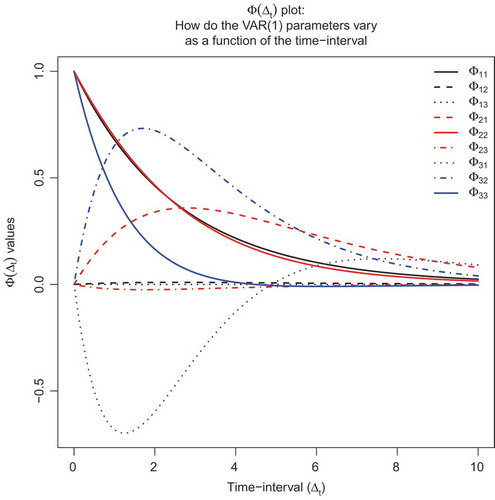
When inspecting the cross-lagged effects, one can see that the ordering for ${\varphi }_{21}$, ${\varphi }_{31}$, and ${\varphi }_{32}$ changes depending on the employed time-interval. At first, the ordering from high to low is: ${\varphi }_{32}$, ${\varphi }_{21}$, and ${\varphi }_{31}$, Then, just before $\mathrm{\Delta }t=6$, the order of ${\varphi }_{32}$ and ${\varphi }_{21}$ changes. Furthermore, at approximately $\mathrm{\Delta }t=7$ and $\mathrm{\Delta }t=9$, the ${\varphi }_{31}$-line crosses that of ${\varphi }_{32}$ and ${\varphi }_{21}$, respectively. Hence, we see misleading conclusion IIb. Consequently, the conclusions about predictive strength depends on the choice of time-interval. Notably, we expect that one mostly wants to compare the counterparts of each cross-lagged effect, as in conclusion type IIa. We can see that ${\varphi }_{31}$ (green dotted line) crosses ${\varphi }_{13}$ (black dotted line). Hence, we see also specifically misleading conclusion IIa.

Furthermore, we also see that for small time-intervals ${\varphi }_{31}$ is negative; whereas, for larger time-intervals (higher than 5) the sign of this effect is positive.⁴ Hence, we see misleading conclusion III. Notably, this change in sign is because each lagged-effect parameter is a nonlinear function both of the time-interval $\mathrm{\Delta }t$ and every other element in the underlying drift matrix A. In terms of interpretation, Deboeck and Preacher (2016) have suggested for this reason that, in a mediation context, the elements of $\varphi (\mathrm{\Delta }t)$ should be interpreted as total effects rather than direct effects. For a further discussion of this issue in the case of more-than-bivariate CT models, see Aalen, Røysland, Gran, and Ledergerber (2012).

In sum, in this example, we can generate misleading conclusions I to III, based on a single tri-variate, stable, first-order process with real eigenvalues.

Other types of conclusions counter-example

Bear in mind that we have dealt with specific types of conclusions that are commonly of interest. One may, for example, also be interested in whether the lagged effect of a variable on itself is greater or smaller than the lagged effect of this variable on another variable. Such a conclusion is time-interval dependent, even in the bivariate case with real, negative eigenvalues. For example, in Figure 2 one can see that at first, ${\varphi }_{11}>{\varphi }_{12}$, but after the time-interval where the black lines cross the ordering reverses (i.e., ${\varphi }_{11}<{\varphi }_{12}$). Thus, some conclusions might be misleading in a bivariate, stable, nonoscillating, first-order system.

Moreover, the conclusions we focus on address comparisons of (cross-)lagged effects with each other (inspecting the ordering of dominance) or with zero (inspecting the sign) and do not address significance testing. Testing whether an autoregressive or cross-lagged parameter is different from zero depends on the chosen time-interval, but not on the time-scale. Hence, when the goal is significance testing, one should definitely use the CTM. Notably, the significance testing result depends on a number of other factors, like sample size. It is possible that in a realistic scenario, further misleading conclusions will occur due to insufficiently precise parameter estimates, or high uncertainty regarding these estimates.

SUMMARY AND RECOMMENDATIONS

When studying time-varying phenomena, progress in any substantive area of interest is dependent on researchers being able to compare the effects estimated in different studies. We showed, in the case of the common CLPM – a DT, first-order model – how results based on other time-intervals, —scales, or from different types of models (i.e., DT vs. CT) can be made comparable and facilitated this with existing R functions.

Additionally, we have shown the exact circumstances under which drawing three common types of conclusions regrading ordering and sign of lagged effects from a CLPM for a particular uniform time-interval is unproblematic. We have shown that this only holds for bivariate, stable, nonoscillating, first-order systems. That is, it is not possible to: (i) find a different dominant autoregression effect; (ii) find a different dominant cross-lagged effect; or (iii) obtain a different sign in cross-lagged effects for such processes. Furthermore, we showed that under these constraints, researchers will draw the same conclusions (regarding types I to III) when they interpret the first-order continuous-time model effect matrix directly rather than the first-order DT effect matrix for a particular interval.

It should be stressed that the conditions for the three ‘common conclusions’ to be not misleading are strict, namely within the first-order systems only the bivariate, stable processes with real eigenvalues. Consequently, in the general case, it might be best advised to inspect the CTM parameter, that is, the drift matrix; either by transforming the results of a DT model or estimating the CTM directly. Namely, the drift matrix A allows for straightforward comparisons between the results of studies which use different time-intervals of measurement, because it represents a time-interval invariant way of expressing the sign and strength of influence between two processes. When comparing two or more studies via the CTM parameter estimate A, one only needs to ensure that you correct for the use of different time-scales (e.g., months vs. weeks), as outlined in Appendix B.

DISCUSSION

A restriction needed for the comparison of two CLPM effect matrices is that within each study all the time-intervals are equally spaced. Note that this is to ensure that the DT model is not a (biased) mixture of parameter estimates for different time-intervals. In certain contexts (e.g., in large-scale panel surveys) this is a more realistic assumption than in others (e.g., in Experience Sampling Method studies). One practical solution to the problem of unequally spaced time-intervals in the estimation of the CLPM is to insert missing data such that the data have (approximately) equal time-intervals, that is, are (approximately) equally-spaced in time. Such a practical solution could thus allow researchers to use the CLPM and compare CLPM results from studies in which time-intervals are (made) approximately equal. We note, however, that this equally-spaced data assumption of the CLPM does not imply that all researchers should collect equally-spaced data. To the contrary, it might be advantageous to use unequal time-intervals to ensure that we have a chance to observe or better estimate oscillating patterns (Voelkle & Oud, 2013, Section 1.2). Additionally, one should then apply the CTM to the unequally spaced data and draw conclusions from the resulting drift matrix.

In this article, we restrict ourselves to first-order processes which display ‘positive autoregression’, that is, systems which can be modelled with first-order CTMs, as specified in this article. That is, first-order DT processes with real, negative eigenvalues cannot be represented by a first-order CTM like specified in Equation 2.

We showed that, only in bivariate, stable, first-order systems in which the eigenvalues of the effect matrix are real, researchers using different uniform time-intervals will not in general come to contradictory conclusions regarding the sign and relative ordering of effects. This can be interesting when, for example, studying one phenomenon in dyads with an observational study such that the intervals are (approximately) equal. However, this finding should not be taken as an argument for examining only bivariate (stable, first-order) relationships. Namely, when a system is truly trivariate and when omitting a relevant variable, the results will be affected accordingly (i.e., the resulting bivariate autoregression matrix will not be a subset of the one obtained by the trivariate model, see Kuiper & Hamaker, n.d.). Thus, to make reliable conclusions, it is necessary to include all relevant variables in your model.

From our results, one can conclude that in the general case, researchers should draw their substantive conclusions on the basis of the drift matrix, rather than the DT effect matrix at a particular time-interval. This can be done in two ways; by indirect or direct estimation of the CTM. The indirect method of CTM estimation consists of first estimating the CLPM and then solving for the underlying drift matrix. However, this method can only be applied under the constraint that the true drift matrix has real eigenvalues (cf. Hamerle et al., 1991; Yue et al., 2016). Notably, in case the drift matrix (estimate) has complex eigenvalues, the drift matrix cannot always be uniquely solved for by the DT effect matrix for a particular interval. Additionally, transformations of $\mathbf{\Phi }(\mathrm{\Delta }t)$ for different time-intervals then are only uniquely defined for multiples of the chosen time-interval $\mathrm{\Delta }t$. Thus, if there is cyclic behavior, direct estimation of the CTM may be more appropriate. One may also wish then to estimate a second-order rather than a first-order differential equation model. Direct estimation of the CTM has numerous other advantages; for example, multilevel CTMs can account for having different time-intervals between measurement both within- and between- participants, as is common in Experience Sampling Method data.⁵

To conclude, we have shown the exact circumstances under which drawing three common types of conclusions regarding the ordering and sign of lagged effects from a CLPM for a particular uniform time-interval is unproblematic. We have shown that this only holds for bivariate, stable, first-order systems in which the eigenvalues of the effect matrix are real. In the more general case, we have shown that taking a CT modeling approach leads to more clarity and describes more accurately (in a time-interval invariant way) how dynamic processes relate to one another.

Additional information

Funding

The work of each of these authors was supported by grants from the Netherlands Organisation for Scientific Research (NWO; Ryan, Onderzoekstalent Grant 406-15-128; Kuiper, VENI Grant 451-16-019).

Notes

¹ Various assumptions about the underlying causal process and model are needed for reliable interpretation of these effects as representing causal quantities. These will not be detailed or critically evaluated in the current article.

² When using another specification of the CTM, it can model first-order DT processes with negative eigenvalues: Fisher (2001) demonstrates this with the use of two continuous-time Ito processes.

³ Often the eigenvectors are chosen such that the sum of the squared elements are 1; e.g., $v_{11}^2+v_{21}^2=1$.

⁴ Oscillating patterns in our first-order processes of interest occur in the case of complex eigenvalues for two or more variables, and can also occur in case of real eigenvalues when inspecting three or more variables, like in our example. When looking at a vector field (see Strogatz, 1994), one can see the differences between these two scenarios; in case of complex eigenvalues, the trajectory is like a spiral.

⁵ One can find specifications of multilevel CTMs in, for instance, Oravecz and Tuerlinckx (2011) and Voelkle and Oud (2013). Various software packages exist to estimate CTMs, for example, the Bayesian Hierarchical Ornstein-Uhlenbeck Model (BHOUM) toolbox package (Oravecz, 2014); CT-SEM (Driver, Voelkle, & Oud, 2017), an R package based on OpenMx and STAN, for modeling continuous-time appropriately; and generalized local linear approximation (GLLA) via OpenMx (Boker, Deboeck, Edler, & Keel, 2010).

⁶ There are multiple methods which can be used to calculate the matrix exponential, also when using the $expm$ package. A more detailed description on these types of methods can be found in Moler and Van Loan (2013).

APPENDIX A

Eigenvalue Decompositions

Based on the eigenvalue decomposition, a (diagonalizable) square matrix A can be written as:

(8) $\mathit{A}=VD{V}^{-1},$(8)

where V is a (nonsingular) matrix containing the eigenvectors of A, and D is a diagonal matrix containing the (distinct) eigenvalues of A.

For A², it holds true that:

(9) ${\mathit{A}}^{\mathbf{2}}=(VD{V}^{-1})(VD{V}^{-1})=V(D{)}^2{V}^{-1},$(9)

By induction, this yields:

(10) ${\mathit{A}}^{\mathit{n}}=V(D{)}^n{V}^{-1},$(10)

for positive reals n and for all reals n when none of the eigenvalues of A are zero. For the interested reader: in case of complex eigenvalues, there does not exist a unique solution when n is not an integer.

Using Equations 8 and 10, it holds true that:

(11) $\begin{array}{rl}& e^{A\mathrm{\Delta }t}=\sum _{l=0}^{\mathrm{\infty }}(\mathrm{\Delta }t{)}^l\frac{{\mathit{A}}^l}{l!}\\ & =\sum _{l=0}^{\mathrm{\infty }}(\mathrm{\Delta }t{)}^l\frac{\mathit{V}{(\mathit{D})}^l{\mathit{V}}^{-1}}{l!}\\ & =\mathit{V}\left(\sum _{l=0}^{\mathrm{\infty }}\frac{{(\mathrm{\Delta }t\mathit{D})}^l}{l!}\right){\mathit{V}}^{-1}\\ & =\mathit{V}{e}^{D\mathrm{\Delta }t}{\mathit{V}}^{-1}.\end{array}$(11)

Notably, there are multiple methods which can be used to calculate the matrix exponential, a more detailed description on these types of methods can be found in Moler and Van Loan (2013).

Note that the eigenvectors for A and $e^{A\mathrm{\Delta }t}$ (= $\mathbf{\Phi }(\mathrm{\Delta }t)$) are the same and that their eigenvalues are related by D versus $e^{\mathit{D}\mathrm{\Delta }t}$ (= ${\mathit{D}}_{\mathbf{\Phi }(\mathit{D}t)}$), where the latter depends on the time-interval. Consequently, it holds that $\mathit{D}=log({\mathit{D}}_{\mathbf{\Phi }(\mathit{D}t)})/\mathrm{\Delta }t$, which is independent of the time-interval.

APPENDIX B

Details on Relating DT and CT

There is only one Φ belonging to one specific A, which can be calculated in R, when using the $expm$ package,⁶ by:

Phi <- expm(A * delta_t)

A DT effect matrix using a time-interval of $d_1$ can be transformed into one as if another time-interval, namely $d_2$, was used, by employing:

$\begin{array}{rl}& \mathbf{\Phi }(d_1)=e^{\mathit{A}{d}_1},\\ & \mathbf{\Phi }(d_2)=e^{\mathit{A}{d}_2}\\ & =e^{\mathit{A}{d}_1\frac{d_2}{d_1}},\mathrm{w}\mathrm{h}\mathrm{i}\mathrm{c}\mathrm{h}\mathrm{y}\mathrm{i}\mathrm{e}\mathrm{l}\mathrm{d}\mathrm{s}:\\ & \mathbf{\Phi }(d_2)=(\mathbf{\Phi }(d_1){)}^{\frac{d_2}{d_1}}\end{array}.$

Thus, one needs to raise the effect to the power $\frac{d_2}{d_1}$. In case $\frac{d_2}{d_1}$ is an integer one can calculate this in R, when using the $expm$ package, by:

Phi_d2 <- Phi_d1

In case the ratio is not integer, one should use the eigenvalue decomposition and take the power of the eigenvalues as stated in Appendix A; R code is available upon request.

An alternative method of comparing DT effects is to convert all of the relevant effects matrices to their underlying continuous-time drift matrix:

(13) $\begin{array}{rl}& \mathit{A}=log(\mathbf{\Phi }(\mathrm{\Delta }t))/\mathrm{\Delta }t\\ & =\mathit{V}(log({\mathit{D}}_{\mathbf{\Phi }(\mathit{D}t)})/\mathrm{\Delta }t){\mathit{V}}^{-1}\end{array}.$(13)

In R, when using the $expm$ package, this can established by:

A <- logm(Phi)/delta_t

Be aware that, also in case of complex eigenvalues, R will give you only one solution, although there are then multiple; more details are given in Appendix E. Therefore, one should always check whether the eigenvalues (of Φ or A) are real-valued or complex; for example, in R by:

eigen(A, sym = FALSE)$values

If one compares CT effect estimates (i.e., As), one should also make an adjustment. Bear in mind that the DT model parameters are time-interval dependent but time-scale independent, this implies that the values of the time-interval invariant A are time-scale dependent. For example, suppose a researcher uses years as the time-scale and that he obtained $\mathbf{\Phi }(\mathrm{\Delta }{t}^{years}=1)=e^{{\mathit{A}}_{years}\cdot 1}$. When he would have set the time-scale to months, he would have obta-ined $\mathbf{\Phi }(\mathrm{\Delta }{t}^{months}=12)=e^{{\mathit{A}}_{months}\cdot 12}.\mathrm{S}\mathrm{i}\mathrm{n}\mathrm{c}\mathrm{e}\mathbf{\Phi }(\mathrm{\Delta }{t}^{years}=1)$ $=\mathbf{\Phi }(\mathrm{\Delta }{t}^{months}=12)$, it holds that $e^{{\mathit{A}}_{months}\cdot 12}=e^{{\mathit{A}}_{years}\cdot 1}$, yielding ${\mathit{A}}_{years}=12\cdot {\mathit{A}}_{months}$. Thus, although the CTM parameter A is time-interval invariant that makes comparisons of studies using different time-intervals easy and straightforward, its values are dependent on the time-scale. Hence, for good comparability of the values of multiple drift matrices one should do this easy, but necessary, transformation:

$\begin{array}{rl}& {\mathit{A}}_{timescale\mathbf{2}}=T^{\ast }{\mathit{A}}_{timescale\mathbf{1}},\\ & with{T}^{\ast }=\frac{time-scale2intermsoftime-scale1}{time-scale1}>0,\end{array}$

with, in the example, $T^{\ast }=\frac{1year}{1month}=\frac{12months}{1month}=12$. Because of this linear relationship with positive constant ($T^{\ast }$), no misleading conclusions are possible for all uni- and multivariate processes when comparing the results of multiple CTMs (assuming the same underlying process). Stated otherwise, the drift matrix obtained for using some time-scale, ${\mathit{A}}_{timescale\mathbf{1}}$, has no different order of magnitude and sign than the one obtained for another one, ${\mathit{A}}_{timescale\mathbf{2}}=T^{\ast }{\mathit{A}}_{timescale\mathbf{1}}$, with $T^{\ast }>0$.

APPENDIX C

Examine the Drift Matrix A

Using the notation from the section starting on page 11 and following Equation 4, we can write:

$\mathit{A}=\frac{1/d_1}{|\mathit{V}|}\left(\begin{array}{c}{v}_{11}\cdot log({\lambda }_{\mathit{1}})\cdot v_{22}-v_{12}\cdot v_{21}\cdot log({\lambda }_{\mathit{2}})\\ \hspace{0.17em}\\ (log({\lambda }_{\mathit{1}})-log({\lambda }_{\mathit{2}}))\cdot v_{21}\cdot v_{22}\end{array}\begin{array}{c}-(log({\lambda }_{\mathit{1}})-log({\lambda }_{\mathit{2}}))\cdot v_{11}\cdot v_{12}\\ \hspace{0.17em}\\ -v_{12}\cdot v_{21}\cdot log({\lambda }_{\mathit{1}})+v_{11}\cdot v_{22}\cdot log({\lambda }_{\mathit{2}})\end{array}\right),$

where $log({\lambda }_1)/d_1=:{\eta }_1$ and $log({\lambda }_2)/d_1=:{\eta }_2$ are the eigenvalues of A. Notably, time-interval $d_1$ appears in the time-interval independent A and its eigenvalues, since the eigenvalues of $\mathbf{\Phi }(d_1)$ (i.e., ${\lambda }_1$ and ${\lambda }_2$) are functions of this: ${\lambda }_1,{\lambda }_2=e^{{\eta }_{1,2}\cdot d_1}$ and ${\lambda }_1^n,{\lambda }_2^n=e^{{\lambda }_{1,2}\cdot d_1\cdot n}=e^{{\eta }_{1,2}\cdot d_2}$.

One can deduce, by looking at the elements $(p,s)$ of both A and $\mathbf{\Phi }(d_1)$, that all three types of misleading results are obtained when the sign of $({\lambda }_1-{\lambda }_2)$ differs from that of $({\eta }_1-{\eta }_2)=(log({\lambda }_1)-log({\lambda }_2))/d_1$ or better, $(log({\lambda }_1)-log({\lambda }_2))$, since $d_1>0$. Thus, to assess whether the three types of misleading conclusions can occur in bivariate, first-order systems based on the use of a different models (DT vs. CT), it suffices to assess whether there exists an ${\lambda }_1$, ${\lambda }_2$ such that, say, ${\lambda }_1>{\lambda }_2$ and $log({\lambda }_1)<log({\lambda }_2)$. Recall that ${\lambda }_1$ and ${\lambda }_2$ are the eigenvalues of $\mathbf{\Phi }(d_1)$. In case of stable, ‘positive autoregression’, first-order systems with real eigenvalues, these lie between 0 and 1. In that case, the sign of $({\lambda }_1-{\lambda }_2)$ never differs from that of $(log({\lambda }_1)-log({\lambda }_2))$. Therefore, misleading conclusions I to III cannot occur in bivariate, stable, first-order systems with real eigenvalues due to the use of a different model (i.e., DT vs. CT). Additionally, this is also true for some bivariate, stable, first-order systems with complex eigenvalues, as is shown in Appendix D.

APPENDIX D

Symmetric Relationships

The symmetric case refers to the case where reciprocal/cross-lagged effects are constrained to be equal, that is, when the upper-diagonal part of the effect matrix ‘equals’ the lower-diagonal part of the effect matrix, that is, when ${\varphi }_{ij}={\varphi }_{ji}$ for all $i,j=1,\dots ,q$. For instance, Figure 1 depicts a symmetric bivariate relationship if ${\varphi }_{12}={\varphi }_{21}$.

When a matrix M is symmetric, it holds that ${\mathit{M}}^{\prime }=\mathit{M}$ and thus that $V^{-1}=V^{\prime }$ (which means that V is orthogonal):

(14) $\begin{array}{c}{\mathit{M}}^{\mathbf{\prime }}\mathbf{=}\mathbf{(}\mathit{V}{\mathit{D}}_{\mathit{M}}{\mathit{V}}^{\mathbf{-}\mathbf{1}}{\mathbf{)}}^{\mathbf{\prime }}\\ =\mathbf{(}V{D}_M{V}^{\prime }{)}^{\prime }\\ =\mathbf{(}{V}^{\prime }{)}^{\prime }{D_M}^{\prime }{V}^{\prime }\\ =\mathit{V}{D}_M{V}^{\prime }\\ =\mathit{V}{D}_M{V}^{-1}\\ =\mathit{M},\end{array}$(14)

using the properties $({\mathit{M}}_{\mathbf{1}}{M}_{\mathbf{2}}{M}_{\mathbf{3}}{)}^{\prime }={M_{\mathbf{3}}}^{\prime }{M_{\mathbf{2}}}^{\prime }{M_1}^{\prime }$, and ${\mathit{D}}^{\prime }=D$ for symmetric or better diagonal matrices D. Since $\mathbf{\Phi }(d_1)$, $(\mathbf{\Phi }(d_1){)}^n$, and A share the same eigenvectors (and only differ in eigenvalues: ${\mathit{D}}_{\mathbf{\Phi }(d_{\mathbf{1}})}$, $({\mathit{D}}_{\mathbf{\Phi }(d_{\mathbf{1}})}{)}^n$, and $\mathit{D}=log({\mathit{D}}_{\mathbf{\Phi }(d_{\mathbf{1}})})/d_1$, respectively), if one of these is symmetric the other two will be as well.

Thus, in case of a symmetric relationship, one will find equal cross-lagged counterparts (i.e., ${\varphi }_{ij}={\varphi }_{ji}$ or ${\alpha }_{ij}={\alpha }_{ji}$ for all $i,j=1,\dots ,q$) irrespective of the chosen time-interval and model. Consequently, misleading conclusion IIa (i.e., the one in terms of cross-lagged counterparts) does not occur. Note that cross-lagged effects that are not each others’ counterparts can cross each other, that is, misleading conclusion IIb can occur. Moreover, misleading conclusions I and III can still occur.

APPENDIX E

Complex Eigenvalues

In case of a $2\times 2$ matrix, complex eigenvalues can be written as:

$\begin{array}{rl}& {\eta }_1=1/2tr(\mathit{A})+\iota 1/2\sqrt{(}4det(\mathit{A})-(tr(\mathit{A}){)}^2)=:\tau +\iota \omega ,\\ & {\eta }_2=\tau -\iota \omega \end{array},$

with $tr(\mathit{A})={\alpha }_{11}+{\alpha }_{22}$, $det(\mathit{A})={\alpha }_{11}{\alpha }_{22}-{\alpha }_{12}{\alpha }_{21}$, ${\iota }^2=-1$ and, by definition, $\omega \ne 0$ (i.e., $(tr(\mathit{A}){)}^2-4det(\mathit{A})<0$). When the eigenvalues are complex and the real part is negative, then the system is oscillating but stable, that is, the system will spiral around the equilibrium along some axes to the equilibrium. Notably, since complex eigenvalues always come in conjugate pairs, a one-variable first-order continuous-time model never shows oscillations. In case of oscillating processes, one may also wish to estimate a second-order rather than a first-order differential equation model.

The eigenvalues for a bivariate $\mathbf{\Phi }(\mathrm{\Delta }t)=e^{A\mathrm{\Delta }t}$, that is, the eigenvalues for a bivariate, ‘positive autoregression’, first-order system are:

$\begin{array}{r}{\lambda }_1=e^{{\eta }_1\mathrm{\Delta }t}=e^{(\tau +\iota \omega )\mathrm{\Delta }t}\\ & =e^{\tau \mathrm{\Delta }t}{e}^{\iota \omega \mathrm{\Delta }t}\\ & =e^{\tau \mathrm{\Delta }t}(cos(\omega \mathrm{\Delta }t)+\iota sin(\omega \mathrm{\Delta }t))\\ & =e^{\tau \mathrm{\Delta }t}cos(\omega \mathrm{\Delta }t)+\iota e^{\tau \mathrm{\Delta }t}sin(\omega \mathrm{\Delta }t)\\ & :=\gamma (\mathrm{\Delta }t)+\iota \theta (\mathrm{\Delta }t),\\ & {\lambda }_2=e^{{\eta }_2\mathrm{\Delta }t}:=\gamma (\mathrm{\Delta }t)-\iota \theta (\mathrm{\Delta }t)\end{array}.$

Hence, if A has complex eigenvalues and thus eigenvectors (i.e., $\omega \ne 0$), the eigenvectors and thus eigenvalues of $\mathbf{\Phi }(\mathrm{\Delta }t)$ are complex as well (i.e, $\theta (\mathrm{\Delta }t)\ne 0$). Since $e^{2\pi \iota n}=1$ for $n=0,\pm 1,\pm 2,\dots$, a specific A leads to only one $\mathbf{\Phi }(\mathrm{\Delta }t)$. On the other hand, since the cosine and sine functions are periodic with $2\pi /\mathrm{\Delta }t$, multiple $\mathbf{A}$s, namely ones with complex eigenvalues and their periodic equivalents, the so-called aliasing matrices (for more details see Hamerle et al., 1991), can lead to the same $\mathbf{\Phi }(\mathrm{\Delta }t)$. Stated otherwise, in case of complex eigenvalues, there is no one-to-one correspondence between $\mathbf{\Phi }(\mathrm{\Delta }t)$ and A if you do not specify additional conditions. Yue et al. (2016) state that there is a one-to-one correspondence between $\mathbf{\Phi }$ and A in case the imaginary parts of all the eigenvalues of A (i.e., $\omega$) lie into $(-\pi /\mathrm{\Delta }t,\pi /\mathrm{\Delta }t)$. If the used sampling frequency is higher than the maximum sampling frequency, other a-priori information about A is required to reduce the number of multiple solutions and/or one needs to search over a collection of matrix logarithms to find the sparsest one, see Yue et al. (2016).

For a DT process to be stable, we need the modulus (i.e., the absolute value) of the eigenvalues of $\mathbf{\Phi }(\mathrm{\Delta }t)$ to be smaller than 1: $\sqrt{\gamma {(\mathrm{\Delta }t)}^2+\theta {(\mathrm{\Delta }t)}^2}<1$. Note that if $\theta (\mathrm{\Delta }t)=0$ and thus if the eigenvalue is real and not complex, this reduces to $\sqrt{\gamma {(\mathrm{\Delta }t)}^2}=\left|\gamma (\mathrm{\Delta }t)\right|<1$, which implies real eigenvalues between −1 and 1. From the equations above, we can deduce that:

$\sqrt{\gamma {(\mathrm{\Delta }t)}^2+\theta {(\mathrm{\Delta }t)}^2}=\sqrt{{(e^{\tau \mathrm{\Delta }t}cos(\omega \mathrm{\Delta }t))}^2+{(e^{\tau \mathrm{\Delta }t}sin(\omega \mathrm{\Delta }t))}^2}$

$=\sqrt{e^{2\tau \mathrm{\Delta }t}{(co{s}^2(\omega \mathrm{\Delta }t))}^2+si{n}^2(\omega \mathrm{\Delta }t){)}^2}=\sqrt{e^{2\tau \mathrm{\Delta }t}}=e^{\tau \mathrm{\Delta }t}.$

Consequently, if the modulus of an eigenvalue of $\mathbf{\Phi }(\mathrm{\Delta }t)$ (belonging to a ‘positive autoregression’, first-order system) is smaller than 1, the real part of the corresponding eigenvalue of A (i.e., $\tau$) is negative, and vice versa. Note that there exist first-order DT processes for which the modulus of the eigenvalues is smaller than one, but for which there is no first-order CT equivalent as specified in Equation 2; namely, stable DT processes that do not exhibit ‘positive autoregression’.

When comparing the order of the complex eigenvalues of $\mathbf{\Phi }(\mathrm{\Delta }t)$ versus A, we have to satisfy twice two conditions, depending on the ordering of the imaginary parts of the two eigenvalues. The first set of two conditions is:

1. $\tau +\iota \omega >\tau -\iota \omega$ if $\omega >-\omega$;

2. $\gamma (\mathrm{\Delta }t)+\iota \theta (\mathrm{\Delta }t)>\gamma (\mathrm{\Delta }t)-\iota \theta (\mathrm{\Delta }t)\leftrightarrow sin(\omega \mathrm{\Delta }t)>$ $sin(\omega \mathrm{\Delta }t)>$ if $\theta (\mathrm{\Delta }t)>-\theta (\mathrm{\Delta }t)$.

These two conditions coincide if $\omega \mathrm{\Delta }t$ lies between 0 and $\pi$ (with a period of $2\pi$), that is, if $\omega$ lies between 0 and $\pi /\mathrm{\Delta }t$ (with a period of $2\pi /\mathrm{\Delta }t$). The second set of two conditions is:

1. $\tau +\iota \omega <\tau -\iota \omega$ if $\omega <-\omega$;

2. $\gamma (\mathrm{\Delta }t)+\iota \theta (\mathrm{\Delta }t)<\gamma (\mathrm{\Delta }t)-\iota \theta (\mathrm{\Delta }t)\leftrightarrow sin(\omega \mathrm{\Delta }t)<$ $-sin(\omega \mathrm{\Delta }t)$ if $\theta (\mathrm{\Delta }t)<-\theta (\mathrm{\Delta }t)$.

These two conditions coincide if $\omega$ lies between $-\pi /\mathrm{\Delta }t$ and 0 (with a period of $2\pi /\mathrm{\Delta }t$). Combined, this leads to the restriction that $\omega$ lies between $-\pi \mathrm{\Delta }t$ and $\pi /\mathrm{\Delta }t$ (with a period of $2\pi /\mathrm{\Delta }t$), which is actually also the condition for which there is a unique correspondence between $\mathbf{\Phi }(\mathrm{\Delta }t)$ and A. Stated otherwise, for ranges of time-intervals $\mathrm{\Delta }t$ for which $\omega$ lies between $-\pi /\mathrm{\Delta }t$ and $\pi /\mathrm{\Delta }t$ (with a period of $2\pi /\mathrm{\Delta }t$), conclusions I to III based on $\mathbf{\Phi }(\mathrm{\Delta }t)$ resemble that of A; however, for the ranges between those, conclusions I to III are misleading.

When comparing the order of the complex eigenvalues of $\mathbf{\Phi }(d_1)$ versus $\mathbf{\Phi }(d_2)$, the conditions for obtaining the same conclusions (of types I to III) are less straightforward. Hence, in some systems with complex eigenvalues, you will not find misleading conclusions I to III and in some you will. However, we do already know from the previous result that if for both $\mathrm{\Delta }t=d_1$ and $\mathrm{\Delta }t=d_2$ it holds that $\omega$ lies between $-\pi /\mathrm{\Delta }t$ and $\pi /\mathrm{\Delta }t$ (with a period of $2\pi /\mathrm{\Delta }t$), that there are no misleading conclusions I to III based on $\mathbf{\Phi }(d_1)$ versus $\mathbf{\Phi }(d_2)$. Importantly, the substantive conclusions I to III then also resemble that based on the underlying A. An example is given in the Misleading Results section in the main text. Notable, there, $\omega =0.5\pi$ lies between $-\pi /\mathrm{\Delta }t$ and $\pi /\mathrm{\Delta }t$ for $\mathrm{\Delta }t$ between 0 and 2 with a period of 2.

References

- Aalen, O., Røysland, K., Gran, J., & Ledergerber, B. (2012). Causality, mediation and time: A dynamic viewpoint. Journal of the Royal Statistical Society: Series A (Statistics in Society), 175(4), 831–861. doi: 10.1111/rssa.2012.175.issue-4
- Bentler, P. M., & Speckart, G. (1981). Attitudes “cause” behaviors: A structrual equation analysis. Journal of Personality and Social Psychology, 40, 226–238. doi: 10.1037/0022-3514.40.2.226
- Boker, S. M. (2002). Consequences of continuity: The hunt for intrinsic properties within parameters of dynamics in psychological processes. Multivariate Behavioral Research, 37(3), 405–422. doi: 10.1207/S15327906MBR3703_5
- Boker, S. M., Deboeck, P., Edler, C., & Keel, P. (2010). Generalized local linear approximation of derivatives from time series. In S. Chow, & E. Ferrar (Eds.), Statistical methods for modeling human dynamics: An interdisciplinary dialogue (pp. 179–212). Boca Raton, FL: Taylor & Francis.
- Boker, S. M., Neale, M., & Rausch, J. (2004). Latent differential equation modeling with multivariate multi-occasion indicators. In O. H. Van Montfort, & A. Satorra (Eds.), Recent developments on structural equation models (pp. 151–174). Dordrecht, the Netherlands: Kluwer Academic.
- Boker, S. M., & Nesselroade, J. R. (2002). A method for modeling the intrinsic dynamics of intraindividual variability: Recovering parameters of simulated oscillators in multi-wave panel data. Multivariate Behavioral Research, 37, 127–160. doi: 10.1207/S15327906MBR3701_06
- Bolger, N., & Laurenceau, J.-P. (2013). Intensive longitudinal methods: An introduction to diary and experience sampling research. New York, NY: The Guilford Press.
- Bringmann, L. F., Vissers, N., Wichers, M., Geschwind, N., Kuppens, P., Peeters, F., … Tuerlinckx, F. (2013). A network approach to psychopathology: New insights into clinical longitudinal data. PLoS ONE, 8, e60188, 1–13. doi: 10.1371/journal.pone.0060188
- Chow, S., Ferrer, E., & Hsieh, F. (2011). Statistical methods for modeling human dynamics: An interdisciplinary dialogue. New York, NY: Routledge.
- Chow, S., Ram, N., Boker, S., Fujita, F., Clore, G., & Nesselroade, J. (2005). Capturing weekly fluctuation in emotion using a latent differential structural approach. Emotion, 5(2), 208–225. doi: 10.1037/1528-3542.5.2.208
- Deary, I. J., Allerhand, M., & Der, G. (2009). Smarter in middle age, faster in old age: A cross-lagged panel analysis of reaction time and cognitive ability over 13 years in the West of Scotland Twenty-07 Study. Psychology and Aging, 24, 40–47. doi: 10.1037/a0014442
- Deboeck, P. R., & Preacher, K. J. (2016). No need to be discrete: A method for continuous time mediation analysis. Structural Equation Modeling: A Multidisciplinary Journal, 23(1), 61–75. doi: 10.1080/10705511.2014.973960
- Driver, C., Voelkle, M., & Oud, H. (2017). ctsem: Continuous time structural equation modelling [Computer software manual]. (R package version 2.4.0). Retrieved from https://cran.r-project.org/web/packages/ctsem/vignettes/hierarchical.pdf
- Finkel, S. E. (1995). Causal analysis with panel data. Thousand Oaks, CA: Sage.
- Fisher, M. (2001). Modeling negative autoregression in continuous time. (http://www.markfisher.net/mefisher/papers/continuousar.pdf)
- Gollob, H. F., & Reichardt, C. S. (1987). Taking account of time lags in causal models. Child Development, 58(1), 80–92. doi: 10.2307/1130293
- Granger, C. W. J. (1969). Investigating causal relations by econometric models and cross-spectral methods. Econometrica, 37, 424–438. doi: 10.2307/1912791
- Hamaker, E. L., Dolan, C. V., & Molenaar, P. C. M. (2005). Statistical modeling of the individual: Rationale and application of multivariate time series analysis. Multivariate Behavioral Research, 40(2), 207–233. doi: 10.1207/s15327906mbr4002_3
- Hamaker, E. L., Kuiper, R. M., & Grasman, R. P. P. P. (2015). A critique of the cross-lagged panel model. Psychological Methods, 20(1), 102–116. doi: 10.1037/a0038889
- Hamerle, A., Nagl, W., & Singer, H. (1991). Problems with the estimation of stochastic differential equations using structural equations model. Journal of Mathematical Sociology, 16(3), 201–220. doi: 10.1080/0022250X.1991.9990088
- Hamilton, J. D. (1994). Time series analysis. Princeton, NJ: Princeton University Press.
- Koval, P., & Kuppens, P. (2012). Changing emotion dynamics: Individual differences in the effect of anticipatory social stress on emotional inertia. Emotion, 12, 256–267. doi: 10.1037/a0024756
- Kuiper, R. M., & Hamaker, E. L. (n.d.). Effect on residuals in time-lagged relationships due to omitted variables: It is time to go continuously.
- Maxwell, S. E., Cole, D. A., & Mitchell, M. A. (2011). Cross-sectional analyses of longitudinal mediation: Partial and complete mediation under an autoregressive model. Multivariate Behavioral Research, 46(5), 816–841. doi: 10.1080/00273171.2011.606716
- Moler, C., & Van Loan, C. (2013). Nineteen dubious ways to compute the exponential of a matrix, twenty-five years later. SIAM Review, 45(1), 3–49. doi: 10.1137/S00361445024180
- Nohe, C., Meier, L. L., Sonntag, K., & Michel, A. (2015). The chicken or the egg? a meta-analysis of panel studies of the relationship between work–Family conflict and strain. Journal of Applied Psychology, 100(2), 522–536. doi: 10.1037/a0038012
- Oravecz, Z. (2014). Bayesian ornstein-uhlenbeck model (boum) toolbox package. Retrieved from https://sites.psu.edu/zitaoravecz/bayesian-ornstein-uhlenbeck-model/
- Oravecz, Z., & Tuerlinckx, F. (2011). The linear mixed model and the hierarchical ornsteinuhlenbeck model: Some equivalences and differences. British Journal of Mathematical and Statistical Psychology, 64, 134–160. doi: 10.1348/000711010X498621
- Oravecz, Z., Tuerlinckx, F., & Vandekerckhove, J. (2009). A hierarchical OrnsteinUhlenbeck model for continuous repeated measurement data. Psychometrika, 74(3), 395–418. doi: 10.1007/S11336-008-9106-8
- Oravecz, Z., Tuerlinckx, F., & Vandekerckhove, J. (2011). A hierarchical latent stochastic differential equation model for affective dynamics. Psychological Methods, 16(4), 468–490. doi: 10.1037/a0024375
- Oud, J. (2002). Continuous time modeling of the cross-lagged panel design. Kwantitatieve Methoden, 69, 1–27.
- Oud, J., & Delsing, M. (2010b). Continuous time modeling of panel data by means of SEM. In K. van Montfort, J. H. L. Oud, A. Satorra (Eds.), Longitudinal research with latent variables. (pp. 201–244). Berlin, Heidelberg: Springer-Verlag.
- Oud, J., & Delsing, M. J. M. H. (2010a). Continuous time modeling of panel data by means of SEM. In K. Van Montefort, J. Oud, & A. Satorra (Eds.), Longitudinal research with latent variables (pp. 201–244). New York, NY: Springer.
- Pelz, D., & Lew, R. (1970). Sociological methodology. In E. Borgatta (Ed.), Heise’s causal model applied. San Francisco, CA: Jossey-Bass.
- R Core Team. (2013). R: A language and environment for statistical computing. R Foundation for Statistical Computing, Vienna, Austria. Retrieved from http://www.R-project.org/
- Reichardt, C. S. (2011). Commentary: Are three waves of data sufficient for assessing mediation? Multivariate Behavioral Research, 46, 842–851. doi: 10.1080/00273171.2011.606740
- Rogosa, D. R. (1980). A critique of cross-lagged correlation. Psychological Bulletin, 88, 245–258. doi: 10.1037/0033-2909.88.2.245
- Ryan, O., Kuiper, R. M., & Hamaker, E. L. (in press). Continuous time modeling in the behavioral and related sciences. In M. C. V. K. V. Montfort, & J. H. L. Oud (Ed.), A continuous time approach to intensive longitudinal data: What, why and how? New York, NY: Springer.
- Schuurman, N. K., Ferrer, E., de Boer-Sonnenschein, M., & Hamaker, E. L. (2016). How to compare cross-lagged associations in a multilevel autoregressive model. Psychological Methods, 21(2), 206–221. doi: 10.1037/met0000062
- Strogatz, S. H. (1994). Nonlinear dynamics and chaos: with applications to physics, biology, chemistry, and engineering. Reading, MA: Addison-Wesley.
- Voelkle, M. C., & Oud, J. H. L. (2013). Continuous time modelling with individually varying time intervals for oscillating and non-oscillating processes. British Journal of Mathematical and Statistical Psychology, 66, 103–126. doi: 10.1111/j.2044-8317.2012.02043.x
- Voelkle, M. C., Oud, J. H. L., Davidov, E., & Schmidt, P. (2012). An SEM approach to continuous time modeling of panel data: Relating authoritarianism and anomia. Psychological Methods, 17(2), 176–192. doi: 10.1037/a0027543
- Yue, Z., Thunberg, J., & Goncalves, J. (2016). Inverse problems for matrix exponential in system identification: system aliasing. Arxiv Preprint arXiv:1605.06973.