On the Power and Performance of a Doubly Latent Residual Approach to Explain Latent Specific Factors in Multilevel-Bifactor-(S-1) Models

Abstract

A doubly latent residual approach (DLRA) is presented to explain latent specific factors in multilevel bifactor-(S-1) models. The new approach overcomes some important limitations of the multiple indicators multiple causes (MIMIC) approach and allows researchers to predict latent specific factors at different levels. The DLRA is illustrated using real data from a large-scale assessment study. Furthermore, the statistical performance and power of the DLRA is examined in a Monte Carlo simulation study. The results show that the new DLRA performs well if more than 50 clusters and more than 10 observations per cluster are sampled. The power to test structural parameters at level 2 was lower than at level 1. To test a medium effect at level 2, we recommend to sample at least 100 clusters with a minimum cluster size of 10. The advantages and limitations of the new approach are discussed and guidelines for applied researchers are provided.

Keywords:

• MIMIC approach
• multilevel bifactor models
• multilevel structural equation models
• simulation study

Bifactor models are gaining increasing attention in psychology (Eid, Geiser, Koch, & Heene, 2017; Koch, Holtmann, Bohn, & Eid, 2017a; Reise, 2012; Wang & Kim, 2017). Originally, Holzinger and Swineford (1937) proposed the bifactor model to separate general and specific components from unsystematic error variance using confirmatory factor analysis. The great flexibility and intuitive appeal of the bifactor model has led many researchers to apply bifactor models to different research designs including longitudinal designs (e.g., latent state-trait modeling, Schermelleh-Engel, Keith, Moosbrugger, & Hodapp, 2004; Steyer, Ferring, & Schmitt, 1992; Steyer, Mayer, Geiser, & Cole, 2015; Steyer, Schmitt, & Eid, 1999), multitrait-multimethod measurement designs (Eid, Lischetzke, & Nussbeck, 2006; Jeon & Rijmen, 2014; Koch, Eid, & Lochner, 2018; Koch, Holtmann, Bohn, & Eid, 2017b) as well as multilevel measurement designs (Gkolia, Koustelios, & Belias, 2018; Koch, Schultze, Burrus, Roberts, & Eid, 2015; Scherer & Gustafsson, 2015; Wang & Kim, 2017). Today, the bifactor model has become an attractive and widely applied method for modeling multidimensional data in psychology (Eid et al., 2017; Reise, 2012).

In the classical bifactor model proposed by Holzinger and Swineford (1937), it is assumed that a general latent factor loads on all indicators measuring the same underlying construct, whereas a latent specific factor just loads on particular indicators that belong to the same facet or domain. Furthermore, it is assumed that the specific factors are mutually uncorrelated as well as uncorrelated with the general factor. The latent specific factors are often referred to as residual factors, representing the reliable part of the observed variables that has been corrected for the influences of the general factor. Due to the orthogonality of general and specific factors, it is possible to decompose the total variance of each observed variable into a general, a specific, and an error component.

A growing body of research is devoted to the analysis of general and specific factors by the inclusion of manifest or latent explanatory variables into the bifactor model (Koch et al., 2017a). Multilevel bifactor models seem to be especially attractive, as they allow researchers to relate explanatory variables to the general and the specific factors at each measurement level. In educational research, researchers often seek to identify key predictor variables for the specific factors (e.g., teacher, wording, or facet-specific effects) using a multilevel bifactor modeling approach (Koch et al., 2015; Scherer & Gustafsson, 2015; Wang, Kim, Dedrick, Ferron, & Tan, 2017). Similarly, psychologists have included external variables into single- and multi-level bifactor models to explain general as well as specific components of self-esteem (DiStefano & Motl, 2006; Tomás, Oliver, Galiana, Sancho, & Lila, 2013), risk-taking (Nicholson, Soane, Fenton-O’Creevy, & Willman, 2005), optimism (Alessandri, Vecchione, Tisak, & Barbaranelli, 2011), leadership performance (Gkolia et al., 2018), teaching quality (Scherer & Gustafsson, 2015), teaching quality (Hindman, Pendergast, & Gooze, 2016), cognitive abilities (Dickinson, Ragland, Gold, & Gur, 2008; Reynolds, Keith, Ridley, & Patel, 2008), psychopathy (Patrick, Hicks, Nichol, & Krueger, 2007), burn-out (Shirom, Nirel, & Vinokur, 2010) and depression (Yang, Tommet, & Jones, 2009).

According to Koch et al. (2017a), explanatory variables cannot be directly linked to the latent factors in the bifactor model if the external variables correlate with both the general and the specific factors. Bifactor models assume orthogonality of general and specific factors. This assumption is, however, violated if a classical multiple indicator multiple cause (MIMIC) approach is used to link explanatory variables to the latent factors in the model. Specifically, the classical MIMIC approach leads to a suppression structure because $X$ (explanatory variable) shares variance with both $G$ (general factor) and $S_k$ (specific factors), whereas $G$ and $S_k$ are assumed to be uncorrelated in the bifactor model. The orthogonality of $G$ and $S_k$ does no longer hold if a common cause (e.g., $X$) is added into the model. As a consequence, the bifactor model is misspecified because it does not represent the original bifactor model with uncorrelated general and specific factors. If the above suppression structure is not properly modeled, researchers must expect parameter bias of the structural coefficients Koch et al. (2017a). Note that the suppression structure will also arise if an explanatory variable is linked to the specific factors and solely correlates with the general factor in the bifactor model. To properly handle the suppression structure and avoid parameter bias, Koch et al. (2017a) proposed two modeling strategies: the multiconstruct bi-factor approach and the residual approach.

The basic idea of the two modeling strategies is to correct the original explanatory variables from unwanted influences of the general factor, when explaining the latent specific effects in the bifactor model. The multiconstruct bi-factor approach is limited to explanatory variables that can be decomposed into two orthogonal components (Koch et al., 2017a). For example, the multiconstruct bifactor approach has been successfully implemented in the context of latent state-trait modeling (Courvoisier, Eid, & Nussbeck, 2007; Hamaker, Kuiper, & Grasman, 2015; Luhmann, Schimmack, & Eid, 2011). In this context, it is common to decompose time-varying covariates into a general (i.e., time-invariant) and a specific (i.e., time-variable) component. In a second modeling step, the general and specific components of the time-varying covariate are linked to the corresponding trait and state factors in the latent state-trait model.

The residual approach is more general than the multiconstruct bifactor approach and can also be used if the explanatory variables cannot be decomposed into two orthogonal components. The residual approach is based on a latent linear regression analysis and requires two modeling steps. First, the general factor $G$ is partialled out from the covariate (e.g., $\eta$) using a latent regression analysis. If the assumption of multivariate normality holds, the residual variable of the latent regression analysis represents the part of the original covariate that is free of (first-order) influences of the general factor and thus may be termed residualized covariate ($\xi$). In a second step, the residualized covariate $\xi$ is used as an independent variable to explain the latent specific factors $S_k$ in the bifactor model. The regression coefficient of a latent specific factor on the residualized covariate can be interpreted as latent partial regression coefficient, representing the link between the specific factor and the covariate while controlling for the general factor. The residual approach circumvents the suppression structure by correcting the covariates from confounding (first-order) influences of the general factor. Following a similar logic, the residual approach can be used to explain the general factor in a bifactor model while controlling for the specific factors.

In this study, we introduce a combination of the doubly latent approach proposed by Marsh et al. (2009) and the residual approach proposed by Koch et al. (2017a). The new approach is termed doubly latent residual approach (DLRA), as it combines the advantages of both approaches. Specifically, the DLRA allows researchers to (a) properly model the previously described suppression structure, (b) simultaneously include multiple explanatory variables at both levels, and (c) account for measurement error as well as sampling error when aggregating level-1 explanatory variables (i.e., doubly latent approach). To examine the statistical performance and power of the DLRA, we present the results of a Monte Carlo simulation study. To the best of our knowledge, no study has yet proposed an adequate transformation method to properly relate explanatory variables to the latent specific factors in multilevel bifactor models. Furthermore, it is not fully clear what sample size is required to explain latent specific effects of different effect sizes in multilevel bifactor models. With this study we aim to fill this gap in current research.

The remainder of the article is organized as follows. First, two versions of multilevel bifactor models are discussed. Second, the DLRA is presented. Third, the DLRA is illustrated using real data from a large-scale educational study to examine the key determinants of teacher effects at the student and the class level. Fourth, the statistical performance and power of the DLRA is examined under a variety of different data constellations in a Monte Carlo simulation study. Finally, the advantages and limitations of the DLRA are discussed and detailed guidelines for applying researchers are provided.

MULTILEVEL BIFACTOR MODELS

According to Eid et al. (2017), two versions of bifactor models can be distinguished: (a) the classical bifactor model that assumes as many specific factors as there are facets in the design and (b) the restricted bifactor model that encompasses a reduced number of specific factors, which will be termed bifactor-(S-1) model in the remainder of the article. In this study, we focus on multilevel bifactor-(S-1) models, as such measurement designs are increasingly applied in practice. In the discussion, we consider ways to properly treat covariates in classical multilevel bifactor models with $S$ specific factors.

A typical example of a bifactor-(S-1) model is a multirater measurement designs, where different types of raters (e.g., teacher report versus student self-report) serve as facets. In educational research, it is quite common that a class teacher is asked to rate all students in a class. As a consequence, teacher and student ratings are nested within higher clusters (e.g., classes). However, student as well as teacher reports are fixed for each particular student in a class and resemble different perspectives on the target-student. Therefore, student and teacher reports cannot easily be replaced by one another. To properly model multilevel research designs with fixed raters that are nested within classes, Koch et al. (2015) proposed a multilevel bifactor-(S-1) model. Originally, the model was developed for the analysis of multilevel-multitrait-multimethod designs with nested structurally different methods (Koch et al. 2015). In this study, we treat raters as facets and consider a minimal multilevel design including two indicators, one construct, and two raters. Later in the article, we extend our measurement design to multiple facets (i.e., 2, 3, or 4 raters).

The basic idea of the multilevel bifactor-(S-1) model proposed by Koch et al. (2015) is to select a reference facet (e.g., student self-report) and contrast the remaining facets (e.g., teacher report) against this reference facet at each measurement level. We recommend researchers to select the most outstanding facet (i.e., the closed approximation to a gold standard) as the reference facet based on previous findings or substantive theory (Geiser, Eid, & Nussbeck, 2008). In the multilevel bifactor-(S-1) model, a reference facet is chosen by modeling $S$ –1 (instead of $S$) specific factors at each measurement level. If, for example, researchers want to select the first facet as the reference facet (e.g., self-report), then the specific factor of the first facet is dropped at each level. The specific factors belonging to the non-reference methods (e.g., teacher report) are defined as latent residual variables of a latent regression analysis, in which the true-score variable of the non-reference methods is regressed on the true-score variable of the reference method. Hence, the latent specific factors in the multilevel bifactor-(S-1) model reflect the reliable part of a non-reference method (e.g., teacher perspective) that is not shared with the reference method (e.g., student perspective) at a particular measurement level. This way, the multilevel bifactor-(S-1) model allows to contrast different facets (e.g., teacher and student perspective) by means of a latent linear regression analysis at each level (cf. Eid, 2000; Eid, Lischetzke, Nussbeck, & Trierweiler, 2003; Koch et al., 2015).

The multilevel bifactor-(S-1) model bears three advantages. First, it enables researchers to contrast different facets (or methods) that do not share a common metric (e.g., self-reports versus objective tests). Second, it allows to define the specific factors as residual factors at each level, which represent the reliable part of a particular facet that is not shared with the general factor at that level. Third, it allows researchers to decompose the true variance of each indicator belonging to a non-reference facet into a level-specific part that is shared with the reference facet (i.e., consistency coefficient) and a level-specific part that is not shared with the reference facet (i.e., specificity coefficient). Figure 1a shows a multilevel bifactor-(S-1) model with common latent factors.

FIGURE 1 Path diagram of a multilevel bifactor-(S-1) model with (a) common latent factors and (b) with additional indicator-specific method factors for a minimal design with two indicators and two facets (here: raters). $Y_{cpik}^W$ = within observed variable ($p$ = person, $c$ = cluster, $i$ = indicator, and $k$ = facet or rater). $G_{c1}^B$ = between latent trait factor. $G_{cp1}^W$ = within latent trait factor. $S_{ck}^B$ = between latent specific factor. $S_{cpk}^W$ = within latent specific factor, $I{M}_{ci}^B$ = between indicator-specific factor. $I{M}_{cpi}^W$ = within indicator-specific factor. ${\epsilon }_{Ycpij}^W$ = within error variable. The mean structure is not shown to avoid clutter.

As can be seen from Figure 1a, the first facet (e.g., students’ self-reports) serves as the reference facet, as no latent specific factor is modeled for the first facet ($k=1$). The corresponding measurement equation for the self-report of a target-student $p$ nested in cluster $c$ can be written as follows:

(1) $Y_{cpi1}^W={\alpha }_{Gi1}^B+{\lambda }_{Gi1}^B{G}_{c1}^B+{\lambda }_{Gi1}^W{G}_{cp1}^W+{\epsilon }_{Ycpi1}^W,$(1)

where $i$ denotes indicator and $k$ represents the facet (here: self-reports; $k$ = 1). The superscripts ($W$= within and $B$ = between) denote the measurement level. According to the Equation (1), each observed variable $Y_{cpi1}^W$ belonging to indicator $i$ of the first facet $k=1$ is decomposed into an additive constant ${\alpha }_{Gi1}^B$, a weighted between general factor ${\lambda }_{Gi1}^B{G}_{c1}^B$, a weighted within general factor ${\lambda }_{Gi1}^W{G}_{cp1}^W$, and an error variable ${\epsilon }_{Ycpi1}^W$. The values of the between general factor $G_{c1}^B$ represent the true scores of the first facet measured at level 2 (e.g., the overall self-reported intrinsic motivation of a particular class). The values of the within general factor reflect the true scores of the first facet measured at the student level (e.g., true self-reported intrinsic motivation of a student corrected for the true average intrinsic motivation of the class). The error variables capture unsystematic error variance at the within level. The observed variables $Y_{cpik}^W$ belonging to indicator $i$ measured by the remaining facets ($k\ne 1$, e.g., teacher reports) are decomposed as follows:

(2) $Y_{cpik}^W={\alpha }_{Gik}^B+{\lambda }_{Gik}^B{G}_{c1}^B+{\lambda }_{Sik}^B{S}_{ck}^B+{\lambda }_{Gik}^W{G}_{cp1}^W+{\lambda }_{Sik}^W{S}_{cpk}^W+{\epsilon }_{Ycpik}^W.$(2)

The specific factors $S_{ck}^B$ and $S_{cpk}^W$ in Equation (2) represent the reliable (between or within) part of a specific facet $k$ (here: teacher reports) that is not shared with the reference facet (here: students’ self-reports). More specifically, the between specific factor $S_{ck}^B$ can be interpreted as teacher effect measured at level 2, that is, the true teacher perspective that is not shared with the student perspective at the class level, whereas $S_{cpk}^W$ denotes the teacher effect measured at level 1, that is, the true teacher perspective that is not shared with the student perspective at the student level. Again, the error variables ${\epsilon }_{Ycpik}^W$ capture unsystematic error variance at the within level.

The above multilevel bifactor-(S-1) model with common latent factors may be too restrictive, especially if additional indicator-specific method effects exist (e.g., wording effects due to positive and negative worded items). To account for additional indicator-specific method effects, the measurement Equations (1) and (2) can be extended in the following way (see also Figure 1b):

(3) $Y_{cpi1}^W=\left(\begin{array}{cc}{\alpha }_{G11}^B+{\lambda }_{G11}^B{G}_{c1}^B+{\lambda }_{G11}^W{G}_{cp1}^W+{\epsilon }_{Ycp11}^W& \mathrm{f}\mathrm{o}\mathrm{r}i=1,\\ {\alpha }_{Gi1}^B+{\lambda }_{Gi1}^B{G}_{c1}^B+{\lambda }_{Gi1}^W{G}_{cp1}^W+& \hspace{0.17em}\\ \\ {\lambda }_{IMi1}^{B}I{M}_{ci}^B+{\lambda }_{IMi1}^{W}I{M}_{cpi}^W+{\epsilon }_{Ycpi1}^W& \mathrm{f}\mathrm{o}\mathrm{r}i\ne 1.\end{array}\right.$(3)

For the remaining facets (i.e., $k\ne 1$), the measurement equation of the observed variables is given by

(4) $Y_{cp1k}^W=\left(\begin{array}{cc}{\alpha }_{G1k}^B+{\lambda }_{G1k}^B{G}_{c1}^B+{\lambda }_{G1k}^W{G}_{cp1}^W+& \hspace{0.17em}\\ {\lambda }_{S1k}^B{S}_{ck}^B+{\lambda }_{S1k}^W{S}_{cpk}^W+{\epsilon }_{Ycp1k}^W& \mathrm{f}\mathrm{o}\mathrm{r}i=1,\\ {\alpha }_{Gik}^B+{\lambda }_{Gik}^B{G}_{c1}^B+{\lambda }_{Gik}^W{G}_{cp1}^W+& \hspace{0.17em}\\ {\lambda }_{Sik}^B{S}_{ck}^B+{\lambda }_{Sik}^W{S}_{cpk}^W+& \hspace{0.17em}\\ \\ {\lambda }_{IMik}^{B}I{M}_{ci}^B+{\lambda }_{IMik}^{W}I{M}_{cpi}^W+{\epsilon }_{Ycpik}^W& \mathrm{f}\mathrm{o}\mathrm{r}i\ne 1.\end{array}\right.$(4)

In Equations (3) and (4), latent indicator-specific factors were specified at both levels. To account for the heterogeneity among the indicators, it is sufficient to specify $i-1$ latent indicator-specific factors. Again, researchers have to select a reference indicator (e.g., $i=1$, positively worded items or parcels) and contrast the remaining indicators (e.g., $i\ne 1$, negatively worded items or parcels) against this refe4rence indicator. The indicator-specific factor $I{M}_{cpi}^W$ captures the reliable part of the negatively worded items that is neither shared with the positively worded items nor with the general or the specific factors at level 1. Similarly, the indicator-specific factors $I{M}_{ci}^B$ capture the heterogeneity among the indicators that is not shared with the general or the specific factors at level 2.

The above multilevel bifactor-(S-1) models allow researchers to decompose the total variance of each observed variable into general, facet-specific, indicator-specific, and error components. Table 1 summarizes the different variance coefficients that can be computed in the multilevel bifactor-(S-1) model with indicator-specific factors. Below we briefly explain the meaning of the most relevant variance coefficients in the model. A detailed discussion of these coefficients can be found in the study by Koch et al. (2015). The consistency coefficients ($Co{n}_B$, $Co{n}_W$) are indicators of the convergent validity between teacher and student reports at each level. The between consistency coefficient $Co{n}_B$ can be interpreted as a measure of rater congruence between student and teacher reports at the between level, whereas $Co{n}_W$ is a measure of the rater congruence at the within level. The total consistency coefficient is the sum of $Co{n}_B$ and $Co{n}_W$ and ranges between 0 and 2. The specificity coefficients ($Sp{e}_B$, $Sp{e}_W$) are the complements of the previously described consistency coefficients and reflect the degree of rater disagreement at each level. In this study, the within and between specificity coefficients will be interpreted as measures of teacher effects at both levels. The total specificity coefficient is the sum of $Sp{e}_B$ and $Sp{e}_W$. The indicator-specificity coefficients ($ISp{e}_B$ and $ISp{e}_W$) are measures of the heterogeneity among the indicators at each level. The true intra-class correlation ($IC{C}_{\tau }$) is defined as ratio of the true between variance to the total true variance of an indicator. Finally, the reliability ($Re{l}_Y$) of an indicator is defined as ratio of the overall variance to the observed variance.

TABLE 1 Variance Components in the Multilevel Bifactor-(S-1) Model with Indicator-Specific Factors

Coefficient	Level	Formula
True score variance	Within	${\sigma }_{W_{\tau }}^2=({\lambda }_{Gik}^W{)}^{2}Var(G_{cp1}^W)+({\lambda }_{Sik}^W{)}^{2}Var(S_{cpk}^W)+({\lambda }_{IMik}^W{)}^{2}Var(I{M}_{cpi}^W)$
	Between	${\sigma }_{B_{\tau }}^2=({\lambda }_{Gik}^B{)}^{2}Var(G_{c1}^B)+({\lambda }_{Sik}^B{)}^{2}Var(S_{ck}^B)+({\lambda }_{IMik}^B{)}^{2}Var(I{M}_{ci}^B)$
	Total	${\sigma }_{T_{\tau }}^2={\sigma }_{W_{\tau }}^2+{\sigma }_{B_{\tau }}^2$
Observed variance	Total	${\sigma }_Y^2={\sigma }_{T_{\tau }}^2+{\sigma }_{\epsilon }^2$
Consistency	Within	$Co{n}_W=({\lambda }_{Gik}^W{)}^{2}Var(G_{cp1}^W)/{\sigma }_{W_{\tau }}^2$
	Between	$Co{n}_B=({\lambda }_{Gik}^B{)}^{2}Var(G_{c1}^B)/{\sigma }_{B_{\tau }}^2$
	Total	$Co{n}_T=Co{n}_W+Co{n}_B$
Specificity	Within	$Sp{e}_W=({\lambda }_{Sik}^W{)}^{2}Var(S_{cpk}^W)/{\sigma }_{W_{\tau }}^2$
	Between	$Sp{e}_B=({\lambda }_{Sik}^B{)}^{2}Var(S_{ck}^B)/{\sigma }_{B_{\tau }}^2$
	Total	$Sp{e}_T=Sp{e}_W+Sp{e}_B$
Indicator-specificity	Within	$ISp{e}_W=({\lambda }_{IMik}^W{)}^{2}Var(I{M}_{cpi}^W)/{\sigma }_{W_{\tau }}^2$
	Between	$ISp{e}_B=({\lambda }_{IMik}^B{)}^{2}Var(I{M}_{ci}^B)/{\sigma }_{B_{\tau }}^2$
	Total	$ISp{e}_T=ISp{e}_W+ISp{e}_B$
Intra-class correlation		$IC{C}_{\tau }={\sigma }_{B_{\tau }}^2/({\sigma }_{B_{\tau }}^2+{\sigma }_{W_{\tau }}^2)={\sigma }_{B_{\tau }}^2/{\sigma }_{T_{\tau }}^2$
Reliability		$Re{l}_Y=({\sigma }_{W_{\tau }}^2+{\sigma }_{B_{\tau }}^2)/{\sigma }_Y^2={\sigma }_{T_{\tau }}^2/{\sigma }_Y^2$

$Note.$ The above coefficients refer to the observed variables belonging to the non-reference facet (i.e., $k\ne 1$). $\sigma$ and $Var(\cdot )$ denote variance, $\tau$ = true score variable, $Y$ = observed variable, $T$ = total, $W$ = within, $B$ = between, $G$ = latent general factor, $S$ = latent specific factor, $IM$ = latent indicator-specific method factor, $\epsilon$ = error variable. $c$ = cluster, $p$ = person nested in cluster, $i$ = indicator, $k$ = facet (reference or non-reference).

DOUBLY LATENT RESIDUAL APPROACH

The DLRA is a combination of the classical doubly latent modeling approach proposed by Marsh et al. (2009) and the residual approach proposed by Koch et al. (2017a). The DLRA requires three modeling steps and is illustrated for one covariate included into a multilevel bifactor-(S-1) model with common latent factors (see Figure 2a) and with indicator-specific latent factors (see Figure 2b).

FIGURE 2 Path diagram of the doubly latent residual approach for a multilevel bifactor-(S-1) model with (a) common latent factors and (b) additional indicator-specific method factors for a minimal design with two indicators and two facets (here: raters). $Y_{cpik}^W$ = within observed variable ($p$ = person, $c$ = cluster, $i$ = indicator, and $k$ = facet or rater). $Z_{cpi}^W$ = covariate measured by indicator $i$ . $G_{c1}^B$ = between latent trait factor. $G_{cp1}^W$ = within latent trait factor. $S_{ck}^B$ = between latent specific factor. $S_{cpk}^W$ = within latent specific factor, $I{M}_{ci}^B$ = between indicator-specific factor. $I{M}_{cpi}^W$ = within indicator-specific factor. ${\epsilon }_{Ycpij}^W$ and ${\epsilon }_{Zcpij}^W$ = within error variable. The mean structure is not shown to avoid clutter.

In the first modeling step, the doubly latent approach by Marsh et al. (2009) is performed by specifying adequate measurement models for the explanatory variables at both levels. Figure 2a illustrates the decomposition of the explanatory variables $Z_{cpi}^W$ into a common latent factor ${\eta }_{cp}^W$ measured at level 1 and a common latent factor ${\eta }_c^B$ measured at level 2, where $p$ = person, $c$ = cluster, and $i$ = indicator:

(5) $Z_{cpi}^W={\mu }_i^B+{\lambda }_{\eta i}^B{\eta }_c^B+{\lambda }_{\eta i}^W{\eta }_{cp}^W+{\epsilon }_{Zcpi}^W.$(5)

In Equation (5), ${\eta }_c^B$ reflects the reliable part of the covariate at level 2 (i.e., true average mean of the covariate), whereas ${\eta }_{cp}^W$ denotes the reliable part of the covariate measured at level 1 (i.e., the deviation of the individual true score from the true average mean of the covariate). For example, ${\eta }_c^B$ may represent the true average level of parental support in a class, whereas ${\eta }_{cp}^W$ may represent the deviation of the true student’s level of parental support from the true average of the class. In practice, the model with common latent factors (see Equation 5) may be too restrictive. A less restrictive model with additional indicator-specific factors at level 2 ${\eta }_{ci}^B$ is depicted in Figure 2b. The measurement equation of this model can be expressed as follows:

(6) $Z_{cpi}^W={\eta }_{ci}^B+{\lambda }_{\eta i}^W{\eta }_{cp}^W+{\epsilon }_{Zcpi}^W.$(6)

The indicator-specific latent factors ${\eta }_{ci}^B$ account for the heterogeneity among the indicators at level 2. To avoid problems of multicollinearity, we generally recommend specifying common (instead of indicator-specific) factors if possible (see Equation 5).

In a second modeling step, the ${\eta }_{cp}^W$ and ${\eta }_{ci}^B$ (see Equation 5) components of the covariate are residualized using the residual approach proposed by Koch et al. (2017a). In case of a multilevel bifactor-(S-1) model with common factors (see Figure 2a), the level-specific components of the covariates are regressed on the corresponding latent general factors measured at each level. The corresponding latent regression equation can be expressed as follows:

(7) ${\eta }_c^B={\gamma }_0^B+{\gamma }_1^B{G}_{c1}^B+{\xi }_c^B,(\mathrm{l}\mathrm{e}\mathrm{v}\mathrm{e}\mathrm{l}2)$(7)

(8) ${\eta }_{cp}^W={\gamma }_1^W{G}_{cp1}^W+{\xi }_{cp}^W.(\mathrm{l}\mathrm{e}\mathrm{v}\mathrm{e}\mathrm{l}1)$(8)

Note that the intercept parameter has been dropped in Equation (8), as the covariate at the within level ${\eta }_{cp}^W$ is defined as zero-mean latent residual variable. The residuals in the above regression equations (see Equations 7 and 8) represent the residualized covariates (${\xi }_c^B$ and ${\xi }_{cp}^W$).

Following a similar logic, researchers can correct the covariates of indicator-specific and general effects if the covariates share variance with both of these factors. The latent regression equations can be expressed as follows (see Figure 2b):

(9) ${\eta }_{c1}^B={\gamma }_{01}^B+{\gamma }_1^B{G}_{c1}^B+{\delta }_1^{B}I{M}_{c2}^B+{\xi }_{c1}^B,(\mathrm{l}\mathrm{e}\mathrm{v}\mathrm{e}\mathrm{l}2)$(9)

(10) ${\eta }_{c2}^B={\gamma }_{02}^B+{\gamma }_2^B{G}_{c1}^B+{\delta }_2^{B}I{M}_{c2}^B+{\xi }_{c2}^B,(\mathrm{l}\mathrm{e}\mathrm{v}\mathrm{e}\mathrm{l}2)$(10)

(11) ${\eta }_{cp}^W={\gamma }_1^W{G}_{cp1}^W+{\delta }_1^{W}I{M}_{cp2}^W+{\xi }_{cp}^W.(\mathrm{l}\mathrm{e}\mathrm{v}\mathrm{e}\mathrm{l}1)$(11)

Again, the intercept parameter has been dropped in Equation (11). The residuals of these latent regression analyses (Equations 9–11) are defined as residualized explanatory variables (${\xi }_{c1}^B$, ${\xi }_{c2}^B$, and ${\xi }_{cp}^W$).

In a third modeling step, the residualized covariates ${\xi }_{c1}^B$, ${\xi }_{c1}^B$ and ${\xi }_{cp}^W$ are used as independent variables in a latent regression analysis to predict the latent specific effects at each level. The latent regression equations can be written as follows (see Figure 2a and 2b):

(12) $S_{c2}^B={\beta }^B{\xi }_c^B+{\zeta }_c^B,(\mathrm{l}\mathrm{e}\mathrm{v}\mathrm{e}\mathrm{l}2)$(12)

(13) $S_{cp2}^W={\beta }_1^W{\xi }_{cp}^W+{\zeta }_{cp}^W.(\mathrm{l}\mathrm{e}\mathrm{v}\mathrm{e}\mathrm{l}1)$(13)

In Equation (12), ${\xi }_c^B$ is a vector containing ${\xi }_{c1}^B$ and ${\xi }_{c2}^B$ . The corresponding latent regression coefficients ${\beta }_1^B$ and ${\beta }_2^B$ are included in the vector ${\beta }^B$. Equation (13) states a linear latent regression of the latent specific factor $S_{cp2}^W$ on the residualized covariate ${\xi }_{cp}^W$ at level 1. The latent regression coefficients in Equations (12) and (13) (i.e., ${\beta }_1^B$, ${\beta }_2^B$, and ${\beta }_1^W$) can be interpreted similary to the partial regression coefficients in ordinary multiple regression analysis. This means that the regression coefficients represent the associations between the specific factors (dependent variables) and the explanatory variables (independent variables) when controlling for general as well as indicator-specific effects at each level. In contrast, the explanatory variables are not residualized in the MIMIC approach, but directly related to the latent factors in the bifactor model. This means that the latent regression coefficients under the MIMIC approach are not corrected for confounding influences of the general and the indicator-specific factors and, thus, may be biased if the covariate also correlates with the general and indicator-specific factors (Koch et al., 2017a).

EMPIRICAL ILLUSTRATION

The DLRA is illustrated using data from the BiKS-8–14 study.¹ The BiKS-8–14 study is a German large-scale assessment study investigating students’ educational development from age 8 to 14 using multiple methods (i.e., objective competence tests, self-reports, teacher reports, as well as parent reports). For a detailed description of the BiKS-8–14 study see Artelt, Blossfeld, Faust, Roßbach, and Weinert (2013). Here, we re-analyzed data from the first measurement wave of the BiKS study and focused exclusively on students’ intrinsic motivation assessed via self-reports and teacher reports. In the BiKS study, each student was rated by his or her class teacher. In total, the data comprised the ratings of 2,365 students (52.33% males; average age = 9.49) from 155 classes (or class teachers) and 82 schools. The data were analyzed using a twolevel bifactor-(S-1) model (Koch et al., 2015). The third for (school) level was not explicitly modeled, but controlled in the analysis using the Mplus option “type = twolevel complex” (Muthén & Muthén, 1998–2017). As a result, the standard errors and fit statistic were adjusted for the clustering in the data (Muthen & Satorra, 1995). In this study, we chose students’ self-reports as the reference facet. The teacher reports served as the non-reference facet. In line with Koch et al. (2015), the non-reference facet was contrasted against the reference method at both levels. The within specific factor represents the unique perspective of the class teacher on a particular student’s intrinsic motivation that is not shared with the student’s self-report (i.e., individual teacher effect). The between specific factor captures the perspective of the class teacher on the class-specific intrinsic motivation corrected for the students’ self-reported intrinsic motivation (i.e., class-specific teacher effect). The general factors in the model represent the students’ self-reported intrinsic motivation measured at level 1 and level 2. In addition, we modeled latent indicator-specific factors to account for the heterogeneity among the indicators at each level (see Figure 1b). The goal of the present study was to (1) examine the congruence between teachers’ and students’ self-reports within and across classes and (2) explain the teacher-specific perspective on students’ intrinsic motivation by relating a residualized explanatory variable (i.e., parental support perceived by the class teacher) to the latent specific factors at each level. The research questions of the present study can be summarized as follows:

1. To what extent do teacher and student ratings overlap within and between classes?

2. To what extent do teachers have a different perspective on students’ intrinsic motivation that is not shared with the students’ self-reports (i.e., amount of teacher effects at each level)?

3. Does parental support perceived by the class teacher explain teacher effects at each level?

The first research question refers to teachers’ judgment accuracy, which can be defined as the congruence between students’ self-reports and teacher reports (Praetorius, Koch, Scheunpflug, Zeinz, & Dresel, 2017). Teachers’ judgment accuracy was examined with regard to the consistency coefficients at both levels (see Table 1). The second research question refers to the amount of teacher effects at each level, which were examined with regard to the specificity coefficients. To answer the third research question, we related the explanatory variable (i.e., parental support perceived by the teacher) to the latent specific factors at each level using the DLRA.

RESULTS

First, we fitted a multilevel bifactor-(S-1) model with common latent factors (see Figure 1a) to the data. This model did not fit the data well, ${\chi }^2$ (6, $N$ = 2365) = 527.70, $p$ < .001, $CFI$ = .82, $RMSEA$ = .19, $SRM{R}_{L1}$ = .01, $SRM{R}_{L2}$ = .13. Second, we fitted the less restrictive multilevel bifactor-(S-1) model with indicator-specific method factors (see Figure 1b). This model fitted the data acceptably well, ${\chi }^2$ (5, $N$ = 2365) = 48.43, $p$ < .001, $CFI$ = .99, $RMSEA$ = .06, $SRM{R}_{L1}$ = .00, $SRM{R}_{L2}$ = .12, and was therefore chosen for the subsequent analyses. In a third step, we related a residualized covariate (i.e., parental support) to the latent specific factors at both levels using the DLRA. An example Mplus code for this final model is provided in Appendix C. Note that we specified common latent factors with regard to the residualized covariate at both levels to avoid problems of multicollinearity. The fit of this explanatory multilevel bifactor-(S-1) model was acceptable, ${\chi }^2$ (15, $N$ = 2365) = 267.72, $p$ < .001, $CFI$ = .96, $RMSEA$ = .08, $SRM{R}_{L1}$ = .03, $SRM{R}_{L2}$ = .12. The averaged intra-class correlations ranged between .11 for students’ self-reports and .25 for teacher reports. The averaged intra-class correlation for the explanatory variable (parental support) was .17. Table 2 summarizes the results of the multilevel bifactor-(S-1) model.

TABLE 2 Consistency, Specificity and Latent Regression Coefficients

Within (student) level
Multilevel bifactor-(S-1) model					Doubly latent residual approach
Item	$Co{n}_W$	$Sp{e}_W$	$ISp{e}_W$	$Rel$	Covariate	B(SE)	β(SE)	$R^2$(SE)
IML1	.09	.91		.90	Parental	0.50${ }^{\ast \ast \ast }$(0.06)	0.60${ }^{\ast \ast \ast }$(0.05)	.36(0.06)
IML2	.08	.85	.06	.73	Support
Between (class) level
Item	$Co{n}_B$	$Sp{e}_B$	$ISp{e}_B$	$IC{C}_{\tau }$	Covariate	B(SE)	β(SE)	$R^2$(SE)
IML1	.04	.96		.24	Parental	0.36${ }^{\ast }$(0.18)	0.44${ }^{n.s.}$ (0.28)	.20(0.25)
IML2	.03	.91	.06	.17	Support

$Note.$ $W$ = within level, $B$ = between level, $Con$ = consistency coefficient, $Spe$ = specificity coefficient, $ISpe$ = indicator-specificity coefficient, $Rel$ = reliability, $IC{C}_{\tau }$ = true intra-class correlation, B = unstandardized regression coefficient, Beta = standardized regression coefficient, $R^2$ = determination coefficient, SE = standard error, ${ }^{n.s}$ = non-significant, ${ }^{\ast \ast \ast }p$ < .001.

Research question 1 and 2 can be answered by means of the consistency and specificity coefficients that were computed at each level (see Table 2). The consistency coefficients of the teacher reports varied between .084 and .090 at level 1 and between .034 and .037 at level 2. This suggests that the congruence (or convergent validity) between student and teacher reported intrinsic motivation was higher at the individual student level than at the class level. Overall, the consistency coefficients were relatively low and corresponded to a latent correlation between student and teacher reports of $r$ = .30 at level 1 and of $r$ = .19 at level 2. These results indicate a relatively low level of convergent validity (or teacher accuracy) at the within and the between level. The specificity coefficients ranged between .851 and .910 at level 1 and between .905 and .963 at level 2 (see Table 2). This shows that a large proportion of true variance of the teacher ratings was due to the unique perspective of the class teacher that was not shared with the students’ self-reports (i.e., teacher effects). Including the residualized covariate (here: parental support), 36% of the interindividual differences in the teacher effects could be explained at level 1 and about 20% of the interindividual differences in the teacher effects could be explained at level 2. The unstandardized regression coefficients of the residualized covariate were positive. This indicates that teachers who perceived the level of parental support as high also tended to overrate students’ intrinsic motivation at each level (i.e., the individual and the class level), when controlling for students’ self-reported intrinsic motivation at each level. The standardized regression coefficient at level 2 was non-significant. This result may be partly explained by a lack of statistical power at level 2. To evaluate the statistical performance and power of the DLRA in greater detail, we conducted a Monte Carlo study.

SIMULATION STUDY

Many applications of multilevel bifactor models involve a relatively low number of level-1 and level-2 observations. Moreover, researchers typically apply multilevel bifactor models that include multiple specific factors at each level. We conducted a simulation study to examine the statistical performance and power of the DLRA under different data constellations.

Results of previous simulation studies suggest that multilevel bifactor-(S-1) models without covariates perform well if at least 50 clusters and more than 10 observations per cluster are sampled (Koch et al., 2015). Other studies indicate that a larger number of clusters (100 or more) may be required to obtain proper parameter and standard error estimates in multilevel structural equation models (MSEMs, Hox, 2010; Julian, 2001). Results of recent simulation studies suggest that the number of level-1 observations per cluster (i.e., cluster size) can reduce standard error bias in longitudinal MSEMs (Koch, Schultze, Eid, & Geiser, 2014). Moreover, studies have shown that the performance of the doubly latent approach is positively related to the amount of information (i.e., number of clusters and the intra-class correlation) that is available with regard to the level-2 construct (Lüdtke, Marsh, Robitzsch, & Trautwein, 2011). Based on these results, we varied the following factors in our simulation study:

1. existence of indicator-specific effects: a) yes b) no

2. number of latent specific factors: 1, 2, or 3

3. effect size in terms of $R^2$ at each level: small effect ($R^2=.05$), medium effect ($R^2=.15$), large effect ($R^2=.35$), huge effect ($R^2=.50$)

4. number of clusters (nL2): 50, 100, 150, 200, 300, and 500

5. cluster size (nL1): 10, 15, 20, and 30

The true intra-class correlation was varied across indicators belonging to different facets (raters) in the present study: $IC{C}_{\tau }$ $\approx$ .10 for self-reports, $IC{C}_{\tau }$ $\approx$ .30 for teacher reports, and $IC{C}_{\tau }$ $\approx$ .20 for the explanatory variable. At each level, we related one explanatory variable to the latent specific factors (1, 2, or 3) using the DLRA. The effect sizes at each level were varied in terms of $R^2$, ranging from .05 (small), .15 (medium), .35 (large), and .50 (huge). The above $R^2$ values correspond to the following standardized regression coefficients of the residualized covariate: ${\beta }_{s1k}\approx$ .224 (small), ${\beta }_{s1k}\approx$ .387 (medium), ${\beta }_{s1k}\approx$ .592 (large), and ${\beta }_{s1k}\approx$ 0.707 (huge). The above regression coefficients were invariant for the within and between model part as well as for both types of bifactor models (i.e., with or without indicator-specific factors). Due to the greater model complexity (i.e. number of freely estimated parameters) of the bifactor model with indicator-specific factors, we expected a less stable performance of the DLRA in case of low sample sizes. The unstandardized regression coefficients of the explanatory variables on the general factors were set to ${\gamma }_1^W$ = 0.935 at level 1 and to ${\gamma }_1^B$ = 1.000 at level 2 in case of bifactor models with common factors (see Figure 2a). In case of indicator-specific factors (see Figure 2b), we chose the following values for the unstandardized regression coefficients: ${\gamma }_1^B$ = ${\delta }_1^B$ = 0.962 and ${\gamma }_1^W$ = ${\delta }_1^W$ = 0.924. The variance of the general factor was set to ${\sigma }_{G_W}^2$ = 8.0 at level 1 and to ${\sigma }_{G_B}^2$ = 1.0 at level 2. The variance of the indicator-specific factors was set to ${\sigma }_{I{M}_W}^2$ = .20 at level 1 and to ${\sigma }_{I{M}_W}^2$ = .08 at level 2. As a consequence of these settings, the variances and the effect sizes of the residualized covariates (${\xi }_{cp}^W$ and ${\xi }_c^B$) were identical in the simulated models with and without indicator-specific factors. A complete list of the parameter settings in the simulation study is provided in Appendix A together with an example Mplus code in Appendix C.

In total, 576 conditions with 500 replications per condition were simulated (i.e., 288,000 data sets). The data were generated using Mplus 8.1 (Muthén & Muthén, 1998–2017) and MplusAutomation (Hallquist & Wiley, 2017) assuming complete data (i.e., no missing values). All models were fitted to the simulated data using robust maximum likelihood (MLR) estimation.

EVALUATION CRITERIA

The statistical performance of the DLRA was examined with regard to the following criteria: (a) rate of convergence, (b) the number of warning messages referring to potential improper solutions, (c) estimation bias and efficiency, and (d) statistical power.

Convergence Rate

In the simulation, we computed the percentage of the simulated models that converged properly after a maximum number of 500 iterations for the Expectation Maximum (EM) algorithm (i.e., Mplus default setting). We expected a larger number of non-converged models in cases of small sample sizes (e.g., nL2 = 50 and nL1 = 10) and in case of bifactor models including additional indicator-specific factors.

Warning Messages and Improper Solutions

Various warning messages were recorded during the simulation study: warning messages referring to (a) $\mathrm{\Psi }$ -problems, (b) $\mathrm{\Theta }$ -problems, (c) computation problems with regard to the standard errors, (d) an ill-conditioned fisher matrix, (e) a saddle point during the estimation. Again, we expected a larger number of warning messages in extreme conditions with low sample size and high model complexity (i.e., including multiple specific factors as well as indicator-specific effects).

Estimation Bias and Efficiency

In the simulation study, we computed the relative parameter estimation bias (peb), the relative standard error estimation bias (seb), the 95% coverage rate (cover), and the mean square error (MSE) as an indicator of efficiency. The relative peb was calculated for each parameter $p$ and then averaged over parameters of the same parameter type $c$ :

(14) $peb({\hat{\theta }}_c)=\frac{1}{n_c}\sum _{c=1}^{n_c}\left|\frac{1}{n_{rep}}\sum _{e=1}^{n_{rep}}({\hat{\theta }}_{pce}-{\theta }_{pc})/{\theta }_{pc}\right|$(14)

Similarly, the relative seb is calculated as follows:

(15) $seb({\hat{\theta }}_c)=\frac{1}{n_c}\sum _{c=1}^{n_c}\left|\frac{1}{n_{rep}}\sum _{e=1}^{n_{rep}}(\hat{s}d{({\hat{\theta }}_{pc})}_e-sd({\hat{\theta }}_{pc}))/sd({\hat{\theta }}_{pc})\right|$(15)

In accordance with previous studies, the values of peb and seb < .10 (10%) were regarded as acceptable (e.g., Koch et al., 2014; Muthén & Muthén, 2002). The 95% coverage is the proportion of replications for which the 95% confidence interval contains the true (or population) parameter value. The MSE is defined as variance of the parameter estimates across all replications plus the square of the bias for that parameter estimates. Again, the 95% coverage rate and the MSE were averaged across parameters of the same parameter type. The coverage and the MSE indicate how well a parameter and its standard error are estimated and were interpreted as a measure of estimation efficiency. Less bias and greater efficiency were expected with increasing sample size at each level.

Power

Finally, we examined the statistical power for explaining latent specific factors under various sample size conditions as well as different model complexity (i.e., number of latent specific factors included in the model). The goal was to provide recommendations to applied researchers for designing future studies with regard to the analysis of specific effects using the DLRA.

RESULTS

Convergence Rate

Model non-convergence was encountered in 52 out of 576 conditions (9.03%). However, none of the simulated conditions showed severe convergence problems (i.e., convergence rate below 50%). Overall, there were only 14 conditions that showed a convergence rate below 90%. Convergence problems were primarily encountered in conditions with high model complexity (e.g., indicator-specific factors) and a low sample size (e.g., nL2 = 50 and nL1 = 10).

Warning Messages and Improper Solutions

From 576 conditions, 12.5% showed warning messages referring to $\mathrm{\Psi }$ -problems, 7.81% referring to estimation problems of the standard errors, 7.81% referring to an ill-conditioned fisher matrix, and 10.76% referring to problems of reaching a saddle point during the estimation. As expected, the majority of these warning messages were encountered in extreme conditions, in which a relatively complex multilevel bifactor-(S-1) model including multiple latent specific factors and indicator-specific factors was fit to small samples (nL2 = 50 and nL1 = 10). Based on these results, we decided to remove the condition with 50 clusters and 10 observations per cluster from further analyses. We did not encounter any warning messages referring to $\mathrm{\Theta }$ -problems in our simulation study. Overall, the results are promising and show that even complex multilevel bifactor-(S-1) models with covariates at each measurement level can be successfully fitted to relatively small samples.

Estimation Bias and Efficiency

Figure 3 shows the averaged relative peb in the simulated multilevel bifactor-(S-1) models with respect to the sample size at both levels.

FIGURE 3 Averaged peb in the simulated multilevel bifactor-(S-1) models. The y-axis shows the averaged peb across all model parameters. The x-axis refers to the number of specific factors in the model. The upper panel denotes the number of cluster (level-2 observations) and the right panel denotes the cluster size (level-1 observations). Bars colored in light gray refer to models with common factors. Bars colored in dark gray refer to model including indicator-specific factors.

As can be seen from Figure 3, the averaged peb values decreased substantially with increasing sample size at level 1 and level 2. The peb values did not exceed the cutoff value of 10%, except for one condition including 50 clusters and 15 observations per cluster. It is worth noting that the averaged peb values fell below the cutoff value when the model included multiple specific factors. A closer inspection revealed that the variance of the indicator-specific factor at level 1 was poorly estimated in the condition with one specific factor, which in turn may have led to the increased bias in the parameter estimates when explaining the latent specific factor at level 1. Notwithstanding, the number of specific factors in the simulated bifactor models had only a negligible effect on the peb values (see Figure 3). In general, the averaged peb values were consistently larger in conditions including indicator-specific factors.

Figure 4 shows the averaged seb values in the simulated multilevel bifactor-(S-1) models with respect to the sample size on level 1 and level 2.

FIGURE 4 Averaged seb in the simulated multilevel bifactor-(S-1) models. The y-axis shows the averaged seb across all model parameters. The x-axis refers to the number of specific factors in the model. The upper panel denotes the number of cluster (level-2 observations) and the right panel denotes the cluster size (level-1 observations). Bars colored in light gray refer to models with common factors. Bars colored in dark gray refer to model including indicator-specific factors.

According to Figure 4, the averaged seb values exceeded the cutoff value of 10% in the following three sample size conditions: (1) 50 clusters with a cluster size of 15, (2) 50 clusters and a cluster size of 20, and (3) 100 clusters with a cluster size of 10. Note that the seb was only greater than 10% when the simulated model included additional indicator-specific factors and one latent specific factor. Again, these results may be partly explained by the fact that the indicator-specific factors are empirically underidentified in these conditions. If multiple specific factors are modeled (see conditions with 2 or 3 specific factors in Figure 4), the indicator-specific factor is identified by at least three indicators, which leads to unbiased standard error estimates. Overall, the results of our simulation study reveal that the parameters and standard errors are well recovered even in relatively small samples (nL2 = 50 and nL1 = 20; nL2 = 100 and nL1 = 10). These results are promising and suggest that the DLRA performs well under a variety of data constellations. We provide a detailed summary of the averaged peb, seb, and MSE values as well as the 95% coverage rate in Table 3. The MSE values and the 95% coverage rate support the above findings.

TABLE 3 Summary of Estimation Bias and Estimation Efficiency for Different Sample Sizes and Models with or without Indicator-Specific Factors

		Model with common factors
Averaged values	Sample size	50	100	150	200	300	500
	10		0.02	0.01	0.01	0.01	0.00
PEB	15	0.03	0.01	0.01	0.01	0.01	0.00
	20	0.03	0.01	0.01	0.01	0.00	0.00
	30	0.02	0.01	0.01	0.00	0.00	0.00
	10		0.03	0.03	0.03	0.03	0.02
SEB	15	0.05	0.03	0.03	0.03	0.03	0.02
	20	0.04	0.03	0.03	0.03	0.03	0.02
	30	0.05	0.03	0.02	0.03	0.02	0.03
	10		0.04	0.03	0.02	0.01	0.01
MSE	15	0.06	0.03	0.02	0.01	0.01	0.01
	20	0.05	0.02	0.02	0.01	0.01	0.00
	30	0.04	0.02	0.01	0.01	0.01	0.00
	10		0.94	0.94	0.95	0.95	0.95
95% Cover	15	0.93	0.94	0.94	0.94	0.95	0.95
	20	0.92	0.94	0.94	0.94	0.94	0.95
	30	0.93	0.94	0.94	0.94	0.95	0.95
		Model with Indicator-Specific Factors
Averaged values	Sample size	50	100	150	200	300	500
	10		0.04	0.02	0.02	0.01	0.01
PEB	15	0.11	0.02	0.02	0.01	0.01	0.01
	20	0.04	0.02	0.01	0.01	0.01	0.01
	30	0.03	0.01	0.01	0.01	0.01	0.00
	10		0.06	0.05	0.03	0.03	0.02
SEB	15	0.09	0.04	0.04	0.03	0.03	0.03
	20	0.06	0.04	0.03	0.03	0.03	0.02
	30	0.05	0.04	0.03	0.03	0.03	0.03
	10		0.17	0.04	0.03	0.02	0.01
MSE	15	9.81	0.04	0.03	0.02	0.01	0.01
	20	0.09	0.03	0.02	0.01	0.01	0.01
	30	0.05	0.02	0.01	0.01	0.01	0.00
	10		0.94	0.94	0.95	0.95	0.95
95% Cover	15	0.93	0.94	0.94	0.94	0.95	0.94
	20	0.93	0.94	0.94	0.94	0.94	0.95
	30	0.92	0.94	0.94	0.94	0.94	0.95

$Note.$ PEB = averaged parameter bias, SEB = averaged standard error bias, MSE = mean square error, 95% Cover = 95% coverage rate. The number of clusters is presented in the columns. The cluster size is presented in the rows.

Statistical Power

The statistical power of DLRA is illustrated in Figure 5 for the standardized regression coefficients at level 1 and in Figure 6 for the standardized regression coefficients at level 2. The statistical power depended on the number of clusters (nL2), the cluster size (nL1), as well as the effect size. However, the number of specific factors in the bifactor model had only little impact on the statistical power of the DLRA approach. A detailed summary of the power analysis is provided in Table B1 in Appendix B.

FIGURE 5 Power of the standardized latent regression coefficients of different effect sizes at the within level. The dotted line denotes a power of .80. The y-axis shows the statistical power of the standardized latent regression coefficients at the within level. The x-axis refers to the number of specific factors in the model. The upper panel denotes the number of cluster (level-2 observations) and the right panel denotes the cluster size (level-1 observations). Small effect = red line. Medium effect = green line. Large effect = blue line. Huge effect = purple line.

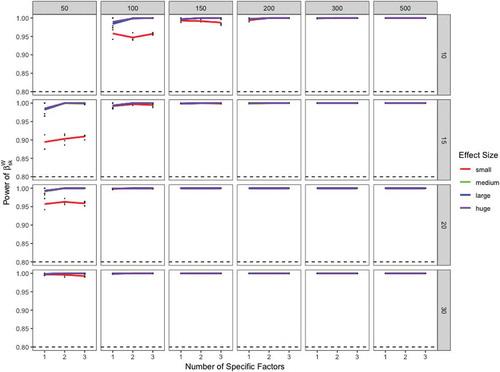
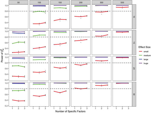
As can be seen from Figure 5, the power at the within level was always greater than 80%. We did not observe a loss in statistical power if multiple specific factors were added in the multilevel bifactor-(S-1) model. This shows the DLRA approach performs well at the within level if at least 50 clusters and more than 10 observations per cluster are sampled. However, the power at the between level fell below 80% in some conditions (see Figure 6). To test a small effect ($R^2=.05$) at the between level with a probability of 80%, researchers must at least sample 300 cluster with 10 observations per cluster. However, the power at the between level was often close to 80% if more than 200 clusters and more than 15 observations per cluster were sampled. To detect larger effects at the between level (i.e., medium, large, or huge effects), a minimal sample size of 100 clusters and 10 observations per cluster should be sampled. Our findings suggest that the number of clusters is a more relevant factor for a sufficient level of statistical power at the between level than the cluster size.

FIGURE 6 Power of the standardized latent regression coefficients of different effect sizes at the between level. The dotted line denotes a power of .80. The y-axis shows the statistical power of the standardized latent regression coefficients at the between level. The x-axis refers to the number of specific factors in the model. The upper panel denotes the number of cluster (level-2 observations) and the right panel denotes the cluster size (level-1 observations). Small effect = red line. Medium effect = green line. Large effect = blue line. Huge effect = purple line.

DISCUSSION

In the present study, we introduced a DLRA to properly explain latent specific factors in multilevel bifactor-(S-1) models. The DLRA combines the advantages of the residual approach by Koch et al. (2017a) and the classical doubly latent approach by Marsh et al. (2009) and overcomes some important limitations of the classical MIMIC approach when explaining latent factors in multilevel bifactor models. Specifically, the DLRA avoids the methodological problems that arise when directly relating explanatory variables to the specific factors in bifactor models (Koch et al., 2017a).

In the DLRA, level-1 explanatory variables are first decomposed into a within and a between component. In a second step, the components are corrected for confounding influences of the latent general factors on each measurement level. The residualized explanatory variables represent the part of the explanatory variables that is not determined by the general factors and thus can be safely related to the specific factors at each level. Researchers must also remove indicator-specific influences from the explanatory variables, if the indicator-specific factors in the model correlate with the explanatory variables.

Another advantage of the DLRA is that it allows researchers to relate explanatory variables to the latent specific factors on multiple measurement levels, while accounting for measurement and sampling error. The DLRA also enables a clearer interpretation of the latent regression coefficients. In the classical MIMIC approach, explanatory variables are not residualized, but directly related to the latent factors in the bifactor model. Similar to multiple regression analysis, the DLRA approach allows researchers to control for the potentially confounding factors in the bifactor model (e.g., influence of the general and/or the indicator-specific factors) when relating the explanatory variables to the latent specific factors in the model. Thus, the DLRA allows researchers to study the relationship between explanatory variables and the latent specific factors at each level when controlling for general and/or indicator-specific effects. Moreover, the residualized explanatory variables in the DLRA are already centered as recommended by many researchers in the context of multilevel modeling (Enders & Tofighi, 2007; Kreft, De Leeuw, & Aiken, 1995). In this article, the DLRA was presented using a latent linear regression analysis. Therefore, the DLRA approach only corrects for linear or first-order dependencies between the general factor and the explanatory variables. To correct for higher-order dependencies, the DLRA needs to be extended to higher-order or nonlinear effects.

The DLRA was illustrated using data from a German large-scale assessment study investigating teacher effects with regard to students’ intrinsic motivation. Our findings suggest that teachers tend to overestimate students’ intrinsic motivation at the within level if teachers also believe that their students receive a high level of parental support, controlling for students’ self-reported level of intrinsic motivation and indicator-specific effects. Similar results were found at the between level, which indicate that teachers tend to overestimate the intrinsic motivation of the entire class if they believe that students in the class receive a high level of parental support (controlling for the students’ self-reported level of intrinsic motivation and indicator-specific effects).

We examined the statistical performance and power of the DLRA in a Monte Carlo simulation study. The results showed that the DLRA performs well in a variety of different data constellations. Overall, the biases in parameter and standard error estimates were negligible and exceeded the cutoff value of 10% only in extreme conditions. The standard errors were slightly biased if a multilevel bifactor-(S-1) model with additional indicator-specific factors was fitted to small samples (i.e., 50 clusters and 15 observations per cluster). To obtain proper parameter and standard errors, we recommend sampling more than 100 clusters and more than 10 observations per cluster. These findings are in line with previous simulation studies in the context of multilevel structural equation modeling (MSEM Hox & Maas, 2001; Julian, 2001; Koch et al., 2014), suggesting that a sufficient number of clusters is required for proper parameter and standard error estimates in MSEM. In terms of statistical power, we recommend researchers to sample a larger number of clusters (e.g., 200–300 clusters) in order to detect small effects at the between level. To detect medium effects at the between level, a sample size of 100 clusters and 10 observations per cluster seems to be sufficient.

In this study, we introduced the DLRA in the context of multilevel bifactor modeling that included a reduced number of specific factors (i.e., $S$ -1 specific factors). It is worth noting that the DLRA can be extended straightforward to traditional multilevel bifactor models that include as many specific factors as there are facets in the design (i.e., $S$ specific factors). In some situations, it may be however more practical to apply the multiconstruct bifactor approach proposed by Koch et al. (2017a) at both levels. For example, a multiconstruct bifactor approach would be beneficial if researchers aim to relate time-varying covariates to the latent factors in a multilevel latent state-trait model in order to explain time-variable and time-invariant interindividual differences at the within (student) and the between (class) level. A multilevel multiconstruct bifactor approach requires that the time-varying covariates are first decomposed into two orthogonal components at each level using the doubly latent approach proposed (Marsh et al., 2009). In a second step, a traditional bifactor structure is used to model the dependent and independent (explanatory) variables at both levels. Finally, the general factors belonging to the explanatory variables can be linked to the general factors belonging to the dependent variables at each level. Similarly, the specific factors belonging to the explanatory variables can be related to the specific factors belonging to the dependent variables at each level. It is important to note that the results of our simulation study cannot be generalized beyond the specific conditions implemented. However, the following recommendations can be derived from our results.

Tip 1: Inspect the First-Order Correlations between the Explanatory Variables and the Latent Factors in the Multilevel Bifactor Model

We recommend researchers to evaluate the first-order correlations between the explanatory variables and the latent factors in the multilevel bifactor model. This way, researchers are able to investigate whether or not a suppression structure is present in the data. The DLRA is recommended whenever the explanatory variables correlate with both the general and the specific factors at a particular level. However, the DLRA is not necessary if the explanatory variables solely correlate with the latent specific factors, but not with the remaining factors in the bifactor model. In these situations, researchers can simply relate the explanatory variables to the latent specific factors in the model and fix the remaining (non-significant) correlations to zero. However, we recommend to center the explanatory variables before the analysis.

Tip 2: Use Multiple Homogeneous Indicators

In the context of the DLRA, we recommend specifying common factors (instead of indicator-specific factors) if possible. Results of our simulation study suggest that the DLRA becomes unstable in case of indicator-specific factors (i.e., larger amount of improper solutions as well as larger bias under the same conditions). Indicator-specific factors pose a problem of multicollinearity, as the latent indicator-specific factors account for the heterogeneity among the indicators. To avoid this problem, we suggest using homogeneous indicators (three indicators per factor). If indicator-specific factors are needed for theoretical or statistical reasons, we suggest to evaluate the first-order correlations as discussed above.

Tip 3: Specify Parsimonious Multilevel Bifactor Models

Our findings suggest that the number of specific factors in the multilevel bifactor-(S-1) model had only little impact on the trustworthiness of the parameter and standard error estimates. In some cases, modeling multiple specific factors was associated with less parameter and standard error bias. Notwithstanding, we recommend specifying parsimonious multilevel bifactor-(S-1) models. Previous simulation studies have suggested that the ratio of observations to the number of freely estimated parameters should exceed 5:1 (Bentler & Chou, 1987) or 10:1 (Bollen, 1989) with regard to classical structural equation models. We recommend a minimal sample size of 50 clusters with 15 observations per cluster. This corresponds to a ratio of 12:1, that is, 750 observations and 62 freely estimated parameters in case of the most complex model. In this simulation study, we have not varied the number of explanatory variables in the model. It can be expected that the statistical power decreases if multiple explanatory variables are added simultaneously into the model.

CONCLUSION

The present study investigated the statistical performance and power of a DLRA when explaining specific factors in multilevel bifactor-(S-1) models. The proposed DLRA overcomes important limitations of the classical MIMIC approach and performs well under a variety of data constellations.

Additional information

Funding

This work was supported by the Deutsche Forschungsgemeinschaft [grant number KO4770/1-1].

Notes

¹ The acronym BiKS stands for educational processes, competence development and selection decisions in preschool and school age.

Appendix A Parameter Settings Used in the Simulation Study

TABLE A1 Population Values of the Structural Parameters Used in the Simulation

			Effect size
			Small		Medium		Large		Huge
Model type	Dependent variable	Parameter label	Within	Between	Within	Between	Within	Between	Within	Between
Model with common factors	$\eta$	${\gamma }_1$	0.935	1.000	0.935	1.000	0.935	1.000	0.935	1.000
		${\sigma }_G^2$	8.000	1.000	8.000	1.000	8.000	1.000	8.000	1.000
		${\sigma }_{\xi }^2$	1.000	1.000	1.000	1.000	1.000	1.000	1.000	1.000
	$S_k$	${\beta }_{1k}$	0.447	0.274	0.775	0.474	1.183	0.725	1.414	0.866
		${\sigma }_{{\zeta }_k}^2$	3.800	1.425	3.400	1.275	2.600	0.975	2.000	0.750
		$co{v}_{{\zeta }_k}$	1.520	0.855	1.360	0.765	1.040	0.585	0.800	0.450
		${\beta }_{s1k}$	0.224	0.224	0.387	0.387	0.592	0.592	0.707	0.707
		$R^2$	0.050	0.050	0.150	0.150	0.350	0.350	0.500	0.500
		$co{r}_{{\zeta }_k}$	0.400	0.600	0.400	0.600	0.400	0.600	0.400	0.600
Model with indicator specific factors	$\eta$	${\gamma }_1$	0.924	0.962	0.924	0.962	0.924	0.962	0.924	0.962
		${\sigma }_G^2$	8.000	1.000	8.000	1.000	8.000	1.000	8.000	1.000
		${\delta }_1$	0.924	0.962	0.924	0.962	0.924	0.962	0.924	0.962
		${\sigma }_{IM}^2$	0.200	0.080	0.200	0.080	0.200	0.080	0.200	0.080
		${\sigma }_{\xi }^2$	1.000	1.000	1.000	1.000	1.000	1.000	1.000	1.000
	$S_k$	${\beta }_{1k}$	0.447	0.274	0.775	0.474	1.183	0.725	1.414	0.866
		${\sigma }_{{\zeta }_k}^2$	3.800	1.425	3.400	1.275	2.600	0.975	2.000	0.750
		$co{v}_{{\zeta }_k}$	1.520	0.855	1.360	0.765	1.040	0.585	0.800	0.450
		${\beta }_{s1k}$	0.224	0.224	0.387	0.387	0.592	0.592	0.707	0.707
		$R^2$	0.050	0.050	0.150	0.150	0.350	0.350	0.500	0.500
		$co{r}_{{\zeta }_k}$	0.400	0.600	0.400	0.600	0.400	0.600	0.400	0.600

$Note.$ ${\delta }_1$= regression coefficient from the indicator-specific factor to the explanatory variable,

${\gamma }_1$= regression coefficient from the general factor to the explanatory variable,

${\sigma }_G^2$ = variance of the general factor, ${\sigma }_{\xi }^2$ = variance of the residualized covariate,

${\sigma }_{IM}^2$ = variance of the indicator-specific factor,

${\beta }_{1k}$ = unstandardized regression coefficient from the residualized covariate to the specific factor,

${\sigma }_{{\zeta }_k}^2$ = residual variance of the specific factor, $co{v}_{{\zeta }_k}$ = covariance between the specific factors,

${\beta }_{s1k}$ = standardized regression coefficient from the residualized covariate to the specific factor,

$R^2$ = coefficient of determination, $co{r}_{{\zeta }_k}$ = correlation between the residuals of the specific factors.

Appendix B Power Analysis

TABLE B1 Power of Statistical Tests of the Standardized Regression Coefficients

			${\beta }_{s1k}^W$						${\beta }_{s1k}^B$
			Number of clusters (nL2)						Number of clusters (nL2)
Specific factors	Effect size $R^2$	cluster size (nL1)	50	100	150	200	300	500	50	100	150	200	300	500
1		10	–	0.96	0.99	0.99	1.00	1.00	–	0.36	0.47	0.62	0.77	0.94
	.05	15	0.89	0.99	1.00	1.00	1.00	1.00	0.25	0.39	0.53	0.67	0.83	0.97
		20	0.96	1.00	1.00	1.00	1.00	1.00	0.33	0.48	0.65	0.75	0.88	0.98
		30	1.00	1.00	1.00	1.00	1.00	1.00	0.40	0.56	0.71	0.82	0.92	0.99
		10	–	0.99	1.00	1.00	1.00	1.00	–	0.77	0.91	0.97	0.99	1.00
	.15	15	0.98	0.99	1.00	1.00	1.00	1.00	0.57	0.84	0.96	0.99	1.00	1.00
		20	0.99	1.00	1.00	1.00	1.00	1.00	0.69	0.91	0.98	0.99	1.00	1.00
		30	1.00	1.00	1.00	1.00	1.00	1.00	0.73	0.95	1.00	1.00	1.00	1.00
		10	–	0.98	1.00	1.00	1.00	1.00	–	0.98	1.00	1.00	1.00	1.00
	.35	15	0.98	0.99	1.00	1.00	1.00	1.00	0.95	1.00	1.00	1.00	1.00	1.00
		20	0.99	1.00	1.00	1.00	1.00	1.00	0.96	1.00	1.00	1.00	1.00	1.00
		30	1.00	1.00	1.00	1.00	1.00	1.00	0.98	1.00	1.00	1.00	1.00	1.00
		10	–	0.99	1.00	1.00	1.00	1.00	–	1.00	1.00	1.00	1.00	1.00
	.50	15	0.99	0.99	1.00	1.00	1.00	1.00	0.99	1.00	1.00	1.00	1.00	1.00
		20	0.99	1.00	1.00	1.00	1.00	1.00	0.99	1.00	1.00	1.00	1.00	1.00
		30	1.00	1.00	1.00	1.00	1.00	1.00	1.00	1.00	1.00	1.00	1.00	1.00
		10	–	0.95	0.99	1.00	1.00	1.00	–	0.35	0.51	0.60	0.77	0.93
2	.05	15	0.90	1.00	1.00	1.00	1.00	1.00	0.26	0.42	0.55	0.68	0.83	0.97
		20	0.96	1.00	1.00	1.00	1.00	1.00	0.32	0.46	0.61	0.72	0.87	0.98
		30	1.00	1.00	1.00	1.00	1.00	1.00	0.37	0.53	0.66	0.79	0.91	0.99
		10	–	1.00	1.00	1.00	1.00	1.00	–	0.80	0.92	0.97	1.00	1.00
	.15	15	1.00	1.00	1.00	1.00	1.00	1.00	0.62	0.87	0.96	0.99	1.00	1.00
		20	1.00	1.00	1.00	1.00	1.00	1.00	0.70	0.91	0.98	1.00	1.00	1.00
		30	1.00	1.00	1.00	1.00	1.00	1.00	0.73	0.95	0.99	1.00	1.00	1.00
		10	–	1.00	1.00	1.00	1.00	1.00	–	0.98	1.00	1.00	1.00	1.00
	.35	15	1.00	1.00	1.00	1.00	1.00	1.00	0.92	1.00	1.00	1.00	1.00	1.00
		20	1.00	1.00	1.00	1.00	1.00	1.00	0.95	1.00	1.00	1.00	1.00	1.00
		30	1.00	1.00	1.00	1.00	1.00	1.00	0.98	1.00	1.00	1.00	1.00	1.00
		10	–	1.00	1.00	1.00	1.00	1.00	–	1.00	1.00	1.00	1.00	1.00
	.50	15	1.00	1.00	1.00	1.00	1.00	1.00	0.98	1.00	1.00	1.00	1.00	1.00
		20	1.00	1.00	1.00	1.00	1.00	1.00	0.99	1.00	1.00	1.00	1.00	1.00
		30	1.00	1.00	1.00	1.00	1.00	1.00	1.00	1.00	1.00	1.00	1.00	1.00
		10	–	0.96	0.99	1.00	1.00	1.00	–	0.40	0.50	0.63	0.79	0.94
3	.05	15	0.91	1.00	1.00	1.00	1.00	1.00	0.28	0.46	0.59	0.71	0.88	0.98
		20	0.96	1.00	1.00	1.00	1.00	1.00	0.31	0.49	0.64	0.76	0.88	0.98
		30	0.99	1.00	1.00	1.00	1.00	1.00	0.37	0.57	0.72	0.82	0.93	0.99
		10	–	1.00	1.00	1.00	1.00	1.00	–	0.77	0.90	0.97	1.00	1.00
	.15	15	1.00	1.00	1.00	1.00	1.00	1.00	0.61	0.87	0.96	1.00	1.00	1.00
		20	1.00	1.00	1.00	1.00	1.00	1.00	0.66	0.91	0.98	1.00	1.00	1.00
		30	1.00	1.00	1.00	1.00	1.00	1.00	0.75	0.95	0.99	1.00	1.00	1.00
		10	–	1.00	1.00	1.00	1.00	1.00	–	0.98	1.00	1.00	1.00	1.00
	.35	15	1.00	1.00	1.00	1.00	1.00	1.00	0.93	1.00	1.00	1.00	1.00	1.00
		20	1.00	1.00	1.00	1.00	1.00	1.00	0.94	1.00	1.00	1.00	1.00	1.00
		30	1.00	1.00	1.00	1.00	1.00	1.00	0.98	1.00	1.00	1.00	1.00	1.00
		10	–	1.00	1.00	1.00	1.00	1.00	–	1.00	1.00	1.00	1.00	1.00
	.50	15	1.00	1.00	1.00	1.00	1.00	1.00	0.98	1.00	1.00	1.00	1.00	1.00
		20	1.00	1.00	1.00	1.00	1.00	1.00	0.99	1.00	1.00	1.00	1.00	1.00
		30	1.00	1.00	1.00	1.00	1.00	1.00	1.00	1.00	1.00	1.00	1.00	1.00

Appendix C Mplus Input Files

Table

DATA:

FILE IS “data.dat”;

VARIABLE:

NAMES ARE

id__LK id__Sch

M__S1n IM__S2m

IM__L1n IM__L2n

Z1 Z2;

MISSING = ALL(−99);

USEVARIABLES ARE

IM__S1n IM__S2m

IM__L1n IM__L2n

Z1 Z2;

CLUSTER = id__LK;

STRATIFICATION = id__Sch;

ANALYSIS:

TYPE = TWOLEVEL COMPLEX;

ESTIMATOR = mlr;

MODEL:

%WITHIN%

Gw BY IM__S1n

IM__S2m

IM__L1n

IM__L2n;

Sw BY IM__L1n

IM__L2n@1;

IMw BY IM__S2m

IM__L2n@1;

Gw WITH Sw@0 IMw@0;

Sw WITH IMw@0;

! Doubly Latent residual approach

! Step 1: Measurement model

Etaw1 by Z1 Z2;

! Step 2: Define residuals

Etaw1 on Gw IMw;

Xiw1 by Etaw1@1;

Etaw1@0;

Xiw1 with Gw@0 IMw@0;

[Xiw1@0];

! Step 3: Explain specific factors

Sw on Xiw1;

%BETWEEN%

Gb BY IM__S1n

IM__S2m@1

IM__L1n

IM__L2n;

Sb BY IM__L1n

IM__L2n@1;

IMb BY IM__S2m

IM__L2n@1;

Gb WITH Sb@0 IMb@0;

Sb WITH IMb@0;

IM__S1n@0;

IM__S2m@0;

IM__L1n@0;

IM__L2n@0;

! Doubly latent residual approach

! Step 1: Measurement model

Etab1 by Z1 Z2;

Z1@0 Z2@0;

! Step 2: Define residuals

Etab1 on Gb IMb;

Xib1 by Etab1@1;

Etab1@0;

Xib1 with Gb@0 IMb@0;

[Xib1@0];

! Step 3: Explain specific factors

Sb on Xib1;

OUTPUT: …;

Montecarlo:

! MULTILEVEL BIFACTOR-(S-1) MODEL WITH

! ONE GENERAL FACTOR AT EACH LEVEL (G)

! TWO SPECIFIC FACTORS AT EACH LEVEL (S)

! TWO INDICATORS PER FACTOR (Y11 to Y23)

! ADDITIONAL INDICATOR-SPECIFIC FACTORS (IM)

! DOUBLY LATENT RESIDUAL APPROACH (z1 and z2)

Names = Y11 Y21

Y12 Y22

Y13 Y23

z1 z2;

NREPS = 500;

Nobservations = 15,000;

NCSIZES = 1;

CSize = 500(30);

SEED = 11,111;

Model Montecarlo:

%WITHIN%

! BIFACTOR STRUCTURE AT LEVEL 1

GW1 by Y11@1

Y21*1

Y12*.4

Y22*.4

Y13*.4

Y23*.4;

SW1 by Y12@1

Y22@1;

SW2 by Y13@1

Y23@1;

IM1 by Y21@1 Y22@1 Y23@1;

FACTOR VARIANCES

GW1*8;

IM1*.20;

! FACTOR INDEPENDENCIES

GW1 with SW1@0 SW2@0 IM1@0;

IM1 with SW1@0 SW2@0;

! MEANS FIXED TO ZERO

[GW1@0];

[SW1@0];

[SW2@0];

[IM1@0];

!ERROR VARIANCES AT LEVEL 1

Y11*2 Y21*2;

Y12*1 Y22*1;

Y13*1 Y23*1;

! ENTER COVARIATE AT LEVEL 1

Zw by z1@1 z2@1;

z1*2 z2*2;

! RESIDUAL APPROACH AT LEVEL 1

Zw on GW1*0.9239364 IM1*0.9239364;

Xi1 by Zw@1;

Xi1*1;

Zw@0;

GW1 IM1 with Xi1@0;

Zw with SW1@0 SW2@0;

[Xi1@0];

! EXPLAIN SPECIFIC EFFECTS AT LEVEL 1

SW1 on Xi1*0.4472136;

SW2 on Xi1*0.4472136;

SW1*3.8;

SW2*3.8;

SW1 with SW2*1.52;

%BETWEEN%

! BIFACTOR STRUCTURE AT LEVEL 2

GB1 by Y11@1

Y21*1

Y12*1

Y22*1

Y13*1

Y23*1;

SB1 by Y12@1

Y22@1;

SB2 by Y13@1

Y23@1;

IM2 by Y21@1 Y22@1 Y22@1;

! FACTOR VARIANCE

GB1*1;

IM2*.08;

! MEANS FIXED TO ZERO

[GB1@0];

[SB1@0];

[SB2@0];

[IM2@0];

! FACTOR INDEPENDENCIES

GB1 with SB1@0 SB2@0 IM2@0;

IM2 with SB1@0 SB2@0;

!ERROR VARIANCES AT LEVEL 2

Y11@0 Y21@0;

Y12@0 Y22@0;

Y13@0 Y23@0;

! INTERCEPTS

[Y11*6 Y21*6];

[Y12*7 Y22*7];

[Y13*7 Y23*7];

! ENTER COVARIATE AT LEVEL 2

Zb by z1@1 z2@1;

z1@0 z2@0;

[z1*5 z2*5];

! RESIDUAL APPROACH AT LEVEL 2

Zb on GB1*0.9622504 IM2*0.9622504;

Xi2 by Zb@1;

Xi2*1;

Zb@0;

GB1 IM2 with Xi2@0;

Zb with SB1@0 SB2@0;

[Xi2@0];

! EXPLAIN SPECIFIC FACTORS AT LEVEL 2

SB1 on Xi2*0.2738613;

SB2 on Xi2*0.2738613;

SB1*1.425;

SB2*1.425;

SB1 with SB2*0.855;

MODEL:

(… as above)

Output: Tech9;

References

- Alessandri, G., Vecchione, M., Tisak, J., & Barbaranelli, C. (2011). Investigating the nature of method factors through multiple informants: Evidence for a specific factor? Multivariate Behavioral Research, 46(4), 625–642. doi:10.1080/00273171.2011.589272
- Artelt, C., Blossfeld, H.-P., Faust, G., Roßbach, H.-G., & Weinert, S. (2013). Bildungsprozesse, Kompetenzentwicklung und Selektionsentscheidungen im vorschulund schulalter [Educational processes, competence development and selection decisions in preschool and school age] (BiKS-8-14). Version: 2 (Tech. Rep.). IQB – Institut zur Qualitätsentwicklung im Bildungswesen. Retrieved from http://doi.org/10.5159/IQB_BIKS_8_14_v2
- Bentler, P. M., & Chou, C.-P. (1987). Practical issues in structural modeling. Sociological Methods & Research, 16, 78–117. doi:10.1177/0049124187016001004
- Bollen, K. A. (1989). Structural equations with latent variables. New York, NY: John Wiley & Sons.
- Courvoisier, D. S., Eid, M., & Nussbeck, F. W. (2007). Mixture distribution latent state-trait analysis: Basic ideas and applications. Psychological Methods, 12, 80–104. doi:http://dx.doi.org/10.1037/1082-989X.12.1.80
- Dickinson, D., Ragland, J. D., Gold, J. M., & Gur, R. C. (2008). General and specific cognitive deficits in schizophrenia: Goliath defeats david? Biological Psychiatry, 64(9), 823–827. doi:10.1016/j.biopsych.2008.04.005
- DiStefano, C., & Motl, R. W. (2006). Further investigating method effects associated with negatively worded items on self-report surveys. Structural Equation Modeling: A Multidisciplinary Journal, 13(3), 440–464. doi:10.1207/s15328007sem1303_6
- Eid, M. (2000). A multitrait-multimethod model with minimal assumptions. Psychometrika, 65(2), 241–261. doi:10.1007/BF02294377
- Eid, M., Lischetzke, T., & Nussbeck, F. (2006). Structural equation models for multitrait-multimethod data. In M. Eid & E. Diener (Eds.), Handbook of multimethod measurement in psychology (pp. 289–299). Washington, DC: American Psychological Association.
- Eid, M., Geiser, C., Koch, T., & Heene, M. (2017). Anomalous results in g-factor models: Explanations and alternatives. Psychological Methods, 22(3), 541–562. doi:http://dx.doi.org/10.1037/met0000083
- Eid, M., Lischetzke, T., Nussbeck, F. W., & Trierweiler, L. I. (2003). Separating trait effects from trait-specific method effects in multitrait-multimethod models: A multiple-indicator CT-C(M-1) model. Psychological Methods, 8(1), 38–60. doi:10.1037/1082-989X.8.1.38
- Enders, C. K., & Tofighi, D. (2007). Centering predictor variables in cross-sectional multilevel models: A new look at an old issue. Psychological Methods, 12, 121–138. doi:http://dx.doi.org/10.1037/1082-989X.12.2.121
- Geiser, C., Eid, M., & Nussbeck, F. W. (2008). On the meaning of the latent variables in the CT-C(M-1) model: A comment on maydeu-olivares and coffman (2006). Psychological Methods, 13(1), 49–57. doi:10.1037/1082-989X.13.1.49
- Gkolia, A., Koustelios, A., & Belias, D. (2018). Exploring the association between transformational leadership and teacher’s self-efficacy in Greek education system: A multilevel sem model. International Journal of Leadership in Education, 21(2), 176–196. doi:10.1080/13603124.2015.1094143
- Hallquist, M., & Wiley, J. (2017). Mplusautomation: Automating mplus model estimation and interpretation [Computer software manual]. Retrieved from https://CRAN.R-project.org/package=MplusAutomation (R package version 0.7)
- Hamaker, E. L., Kuiper, R. M., & Grasman, R. P. (2015). A critique of the cross-lagged panel model. Psychological Methods, 20, 102–116. doi:http://dx.doi.org/10.1037/a0038889
- Hindman, A. H., Pendergast, L. L., & Gooze, R. A. (2016). Using bifactor models to measure teacher–Child interaction quality in early childhood: Evidence from the caregiver interaction scale. Early Childhood Research Quarterly, 36, 366–378. doi:10.1016/j.ecresq.2016.01.012
- Holzinger, K. J., & Swineford, F. (1937). The bi-factor method. Psychometrika, 2(1), 41–54. doi:10.1007/BF02287965
- Hox, J. J. (2010). Multilevel analysis techniques and applications (2nd ed.). New York, NY: Routledge.
- Hox, J. J., & Maas, C. J. (2001). The accuracy of multilevel structural equation modeling with pseudobalanced groups and small samples. Structural Equation Modeling: A Multidisciplinary Journal, 8(2), 157–174. doi:10.1207/S15328007SEM0802_1
- Jeon, M., & Rijmen, F. (2014). Recent developments in maximum likelihood estimation of mtmm models for categorical data. Frontiers in Psychology, 5, 269. doi:10.3389/fpsyg.2014.00269
- Julian, M. W. (2001). The consequences of ignoring multilevel data structures in nonhierarchical covariance modeling. Structural Equation Modeling: A Multidisciplinary Journal, 8(3), 325–352. doi:10.1207/S15328007SEM0803_1
- Koch, T., Holtmann, J., Bohn, J., & Eid, M. (2017b). Multitrait-multimethod-analysis. In V. Zeigler-Hill & T. Shakelford (Eds.), Encyclopedia of personality and individual differences. Berlin, Germany: Springer.
- Koch, T., Eid, M., & Lochner, K. (2018). Multitrait-multimethod-analysis: The psychometric foundation of CFA-MTMM models. In P. Irwing, T. Booth, & D. Hughes (Eds.), The wiley handbook of psychometric testing: A multidisciplinary reference on survey, scale and test development. London, UK: Wiley-Blackwell.
- Koch, T., Holtmann, J., Bohn, J., & Eid, M. (2017). Explaining general and specific factors in longitudinal, multimethod, and bifactor models: Some caveats and recommendations. Psychological Methods. Advance online publication. doi:10.1037/met0000146
- Koch, T., Schultze, M., Burrus, J., Roberts, R. D., & Eid, M. (2015). A multilevel CFA-MTMM model for nested structurally different methods. Journal of Educational and Behavioral Statistics, 40(5), 477–510. doi:10.3102/1076998615606109
- Koch, T., Schultze, M., Eid, M., & Geiser, C. (2014). A longitudinal multilevel CFA-MTMM model for interchangeable and structurally different methods. Frontiers in Quantative Psychology and Measurement, 5:311. doi:10.3389/fpsyg.2014.00311
- Kreft, I. G., De Leeuw, J., & Aiken, L. S. (1995). The effect of different forms of centering in hierarchical linear models. Multivariate Behavioral Research, 30, 1–21. doi:10.1207/s15327906mbr3001_1
- Lüdtke, O., Marsh, H. W., Robitzsch, A., & Trautwein, U. (2011). A 2 × 2 taxonomy of multilevel latent contextual models: Accuracy–Bias trade-offs in full and partial error correction models. Psychological Methods, 16(4), 444–467. doi:10.1037/a0024376
- Luhmann, M., Schimmack, U., & Eid, M. (2011). Stability and variability in the relationship between subjective well-being and income. Journal of Research in Personality, 45, 186–197. doi:10.1016/j.jrp.2011.01.004
- Marsh, H. W., Lüdtke, O., Robitzsch, A., Trautwein, U., Asparouhov, T., Muthén, B., & Nagengast, B. (2009). Doubly-latent models of school contextual effects: Integrating multilevel and structural equation approaches to control measurement and sampling error. Multivariate Behavioral Research, 44(6), 764–802. doi:10.1080/00273170903333665
- Muthen, B. O., & Satorra, A. (1995). Complex sample data in structural equation modeling. Sociological methodology, 267–316.
- Muthén, L. K., & Muthén, B. O. (1998- 2017). Mplus user‘s guide (8th ed.). Los Angeles, CA: Muthén & Muthén.
- Muthén, L. K., & Muthén, B. O. (2002). How to use a monte carlo study to decide on sample size and determine power. Structural Equation Modeling: A Multidisciplinary Journal, 9(4), 599–620. doi:10.1207/S15328007SEM0904_8
- Nicholson, N., Soane, E., Fenton-O’Creevy, M., & Willman, P. (2005). Personality and domain-specific risk taking. Journal of Risk Research, 8(2), 157–176. doi:10.1080/1366987032000123856
- Patrick, C. J., Hicks, B. M., Nichol, P. E., & Krueger, R. F. (2007). A bifactor approach to modeling the structure of the psychopathy checklist-revised. Journal of Personality Disorders, 21(2), 118–141. doi:10.1521/pedi.2007.21.2.118
- Praetorius, A.-K., Koch, T., Scheunpflug, A., Zeinz, H., & Dresel, M. (2017). Identifying determinants of teachers’ judgment (in) accuracy regarding students’ school-related motivations using a bayesian cross-classified multi-level model. Learning and Instruction, 52, 148–160. doi:10.1016/j.learninstruc.2017.06.003
- Reise, S. P. (2012). The rediscovery of bifactor measurement models. Multivariate Behavioral Research, 47(5), 667–696. doi:10.1080/00273171.2012.715555
- Reynolds, M. R., Keith, T. Z., Ridley, K. P., & Patel, P. G. (2008). Sex differences in latent general and broad cognitive abilities for children and youth: Evidence from higher-order mg-macs and mimic models. Intelligence, 36(3), 236–260. doi:10.1016/j.intell.2007.06.003
- Scherer, R., & Gustafsson, J.-E. (2015). Student assessment of teaching as a source of information about aspects of teaching quality in multiple subject domains: An application of multilevel bifactor structural equation modeling. Frontiers in Psychology, 6 1550 Retrieved from https://www.frontiersin.org/article/10.3389/fpsyg.2015.01550 doi:10.3389/fpsyg.2015.01550
- Schermelleh-Engel, K., Keith, N., Moosbrugger, H., & Hodapp, V. (2004). Decomposing person and occasion-specific effects: An extension of latent state-trait (LST) theory to hierarchical LST models. Psychological Methods, 9(2), 198–219. doi:10.1007/s10802-011-9547-x
- Shirom, A., Nirel, N., & Vinokur, A. D. (2010). Work hours and caseload as predictors of physician burnout: The mediating effects by perceived workload and by autonomy. Applied Psychology, 59(4), 539–565. doi:10.1111/j.1464-0597.2009.00411.x
- Steyer, R., Ferring, D., & Schmitt, M. J. (1992). States and traits in psychological assessment. European Journal of Psychological Assessment, 8(2), 79–98.
- Steyer, R., Mayer, A., Geiser, C., & Cole, D. A. (2015). A theory of states and traits—Revised. Annual Review of Clinical Psychology, 11(1), PMID: 25062476, 71–98. doi:10.1146/annurev-clinpsy-032813-153719
- Steyer, R., Schmitt, M., & Eid, M. (1999). Latent state-trait theory and research in personality and individual differences. European Journal of Personality, 13(5), 389–408. doi:10.1002/(SICI)1099-0984(199909/10)13:53.0.CO;2-A
- Tomás, J. M., Oliver, A., Galiana, L., Sancho, P., & Lila, M. (2013). Explaining method effects associated with negatively worded items in trait and state global and domain-specific self-esteem scales. Structural Equation Modeling: A Multidisciplinary Journal, 20(2), 299–313. doi:10.1080/10705511.2013.769394
- Wang, Y., & Kim, E. S. (2017). Evaluating model fit and structural coefficient bias: A Bayesian approach to multilevel bifactor model misspecification. Structural Equation Modeling: A Multidisciplinary Journal, 24(5), 699–713. doi:10.1080/10705511.2017.1333910
- Wang, Y., Kim, E. S., Dedrick, R. F., Ferron, J. M., & Tan, T. (2017). A multilevel bifactor approach to construct validation of mixed-format scales. Educational and Psychological Measurement, 78, 253–271. doi:10.1177/0013164417690858
- Yang, F. M., Tommet, D., & Jones, R. N. (2009). Disparities in self-reported geriatric depressive symptoms due to sociodemographic differences: An extension of the bi-factor item response theory model for use in differential item functioning. Journal of Psychiatric Research, 43(12), 1025–1035. doi:10.1016/j.jpsychires.2008.12.007