Cross-Level Invariance in Multilevel Factor Models

Abstract

When modeling latent variables at multiple levels, it is important to consider the meaning of the latent variables at the different levels. If a higher-level common factor represents the aggregated version of a lower-level factor, the associated factor loadings will be equal across levels. However, many researchers do not consider cross-level invariance constraints in their research. Not applying these constraints when in fact they are appropriate leads to overparameterized models, and associated convergence and estimation problems. This simulation study used a two-level mediation model on common factors to show that when factor loadings are equal in the population, not applying cross-level invariance constraints leads to more estimation problems and smaller true positive rates. Some directions for future research on cross-level invariance in MLSEM are discussed.

Keywords:

• cross-level invariance
• multilevel CFA
• multilevel SEM

In educational and psychological research, data often have a multilevel structure, such as data from children in classrooms, employees in departments, or individuals in countries. Such data structures allow for the investigation of hypotheses at different levels using multilevel structural equation modeling (MLSEM). We limit our presentation to two-level structures of individuals (Level 1 or the within-level) in clusters (Level 2 or the between-level). MLSEM allows for different models for variances and covariances of within-cluster differences and between-cluster differences by decomposing the observed variables into a within component and a between component (Muthén, 1989, 1994; Schmidt, 1969). Given the multivariate response vector y_ij, with scores from subject i in cluster j, the scores are decomposed into means (μ_j), and individual deviations from the cluster means (η_ij):

(1) ${\mathbf{y}}_{ij}={\mu }_j+{\eta }_{ij}$(1)

where μ_j and η_ij are independent. The overall covariances of y_ij (Σ_TOTAL) can be written as the sum of the covariances of these two components:

(2) $\begin{array}{rl}& {\mathbf{\Sigma }}_{\mathrm{T}\mathrm{O}\mathrm{T}\mathrm{A}\mathrm{L}}=\mathrm{C}\mathrm{O}\mathrm{V}\left({\mu }_{\mathrm{j}},{\mu }_{\mathrm{j}}\right)+\mathrm{C}\mathrm{O}\mathrm{V}\left({\eta }_{\mathrm{i}\mathrm{j}},{\eta }_{\mathrm{i}\mathrm{j}}\right)\\ & ={\mathbf{\Sigma }}_{BETWEEN}+{\mathbf{\Sigma }}_{WITHIN}\end{array}$(2)

One can postulate separate models for Σ_BETWEEN and Σ_WITHIN. This model specification is denoted the within/between formulation (Muthén, 1989, 1994), and implies random intercepts for all observed variables. The observed variables can have variance at one or both of the levels in two-level data. For example, in data from children in school classes, the variable ‘Teacher gender’ only has variance at Level 2, since all children in the same school class share the same teacher. The gender of the child varies within school classes, and will have variance at Level 1, but not at Level 2, in cases where the distribution of boys and girls is equal across classes. In practice, variables that have variance at Level 1, often also have variance at Level 2. For example, children’s scores on a mathematical ability test may differ across different children from the same school class (Level 1), while the classroom average test scores are also likely different (Level 2).

Preacher, Zyphur, and Zhang (2010) showed how MLSEM can be used for testing mediation hypotheses with two-level nested data. The MLSEM framework allows the estimation of mediation models in which each of the variables involved can be present on Level 1, Level 2, or both. In contrast, standard multilevel modeling only allows the analysis of mediation models where the mediator and outcome variables are Level 1 variables. Moreover, MLSEM makes it possible to evaluate mediational hypotheses on latent variables.

Despite the clear advantages of MLSEM, two issues warrant attention when working with multilevel factor models. First, one should carefully think about the interpretation of the common factors at the different levels, and use the measurement model that justifies the conclusions drawn about the latent variables (Stapleton, Yang, & Hancock, 2016). Second, one should minimize estimation and convergence problems where possible, by using models that are not overly complex. Cross-level invariance constraints on factor loadings in practice often prevent interpretational as well as estimation problems. The goal of this study is therefore to evaluate the effect of not applying cross-level invariance constraints in situations where these constraints are actually needed. Before presenting the simulation study, we discuss the interpretational and estimation issues associated with cross-level invariance constraints on factor loadings in more detail.

Interpretation of common factors at different levels in MLSEM

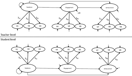
The technical possibility to fit different models to Σ_BETWEEN and Σ_WITHIN, has led to applications of MLSEM where different factor structures are applied to the different levels. In a review of reporting practices of multilevel factor analyses, Kim, Dedrick, Cao, and Ferron (2016) found that 31% of the studies reported a different number of factors at the two levels. However, models with different numbers of factors at different levels are hard to interpret (Hox, Moerbeek & van der Schoot, 2017). The appropriate way of modeling latent variables in multilevel SEM depends on the theoretical meaning of the latent variable (Stapleton et al., 2016). In situations where the within- and between-factors reflect the within- and between-components of the same latent variable, the same factor structure applies at the two levels, and the factor loadings will be equal across levels (Asparouhov & Muthén, 2012; Mehta & Neale, 2005; Rabe-Hesketh, Skrondal & Pickels, 2004). For example, suppose that researchers are interested in how teacher-student relations affect student achievement through student engagement, and that each of these constructs is measured using three appropriate items administered to several students per teacher. The hypothesized model is depicted in Figure 1. All variables have variance at the student-level as well as at the teacher-level, meaning that there is a potential mediational effect at each level. In the taxonomy of Preacher et al. this scenario would be called mediation in a 1–1–1 design. The mediational hypotheses of interest could be as follows. Students who have better relations with their teacher than classmates, may be more engaged in school work than their classmates, and subsequently achieve better than their classmates. At the same time, teachers who have on average better relations with their students than other teachers, may have students that are on average more engaged in school, and therefore on average achieve higher than students of other teachers. In order to evaluate the two mediational effects on the within- and between-components of the three constructs of interest, the factors should be modeled with equal factor loadings across levels. This way, the observed variables are affected by the within- and between-components of the same latent variable at the two levels.

FIGURE 1 Example of a 1-1-1 mediational design on common factors representing teacher-student relations, student engagement, and student achievement.

These types of constructs, which are frequently observed in the literature (Kim et al., 2016), are labeled “configural constructs” in a recent taxonomy by Stapleton et al. (2016). Although often needed, the requirement of cross-level invariance is commonly overlooked, leading to researchers giving the same name to the factors at two levels, without actually modeling the factors accordingly. In a recent overview of 72 applications of multilevel factor analysis, Kim et al. found that cross-level invariance was tested in only 6 of the 72 applications, and that explicit discussions of how researchers conceptualize the constructs are generally lacking. Kim et al. stress that cross-level invariance is essential for the construct validity of configural constructs, and call for more attention to cross-level invariance in applications of multilevel factor analysis.

It should be noted that the cross-level invariance constraints needed for correct interpretation of configural constructs apply to factor loadings only. All other parameters can be different across levels. By imposing cross-level invariance constraints, the covariance structure on the between-level is identified using the identification constraint at the within-level (or vice versa). This implies that if the factor variance is fixed for identification at one level, the factor variance at the other level can (and should) be freely estimated. Regression effects between latent variables may also be different across levels, allowing for contextual effects (Marsh, Lüdtke, Robitzsch, Trautwein, Asparouhov, Muthén & Nanengast, 2009). Residual variance is likely to be smaller at the between-level than at the within-level. It is actually quite common to find zero residual variance at the between-level for at least some variables, since strong factorial invariance across clusters implies absence of residual variance at the between-level in a model with cross-level invariance (Jak & Jorgensen, 2017; Jak, Oort, & Dolan, 2013; Muthén, 1990; Rabe-Hesketh et al., 2004). Stapleton et al. (2016) propose an even more general model for configural constructs in which the variance of the within-cluster latent variable can be cluster specific. This model, and more complex models in which all item parameters can be random across clusters (e.g., De Jong, Steenkamp, & Fox, 2007), can however only be estimated with Bayesian methods. In this study, we consider models with random intercepts only, so that all models can be estimated in the frequentist framework.

Estimation problems in MLSEM

MLSEM is notorious for estimation problems. Especially in cases where the number of clusters is small, and/or the variance at level 2 is small, non-converged and inadmissible solutions are frequently observed (Jak, Oort, & Dolan, 2014; Li & Beretvas, 2013; Ludtke, Marsh, Robitzsch & Trautwein, 2011). One solution that is regularly applied to limit the number of parameters to be estimated, is applying cross-level invariance on the factor loadings (Depaoli & Clifton, 2015; Gonzalez-Roma & Hernandez, 2017). This practice shows that, in addition to solving interpretational issues, invariance of factor loadings across levels also facilitates estimation of model parameters. Interestingly, applying these constraints has even been found to improve convergence, without leading to estimation bias, in conditions where the population factor loadings were unequal across levels (Kim & Cao, 2015).

The current study

To recapitulate, there are two reasons why researchers should evaluate cross-level invariance of factor loadings in MLSEM. The main reason is that it is a necessary constraint to enable the interpretation of the between-factor and the within-factor as the within- and between-components of the same common factor. The second reason is that in many situations, not-applying cross-level invariance constraints leads to an overparameterized model, and associated estimation problems. Previous simulation studies never explicitly focused on the effect of (not) applying cross-level invariance constraints in multilevel factor models. Some studies generated data with equal factor loadings, but did not apply cross-level constraints in the analysis (Kim, Yoon, Wen, Luo, & Kwok, 2015; Li & Beretvas, 2013), others generated data with different numbers of factors or different factor loadings across levels (Hox, Maas, & Brinkhuis, 2010; Lee & Cho, 2017), or focused on comparing frequentist and Bayesian estimation methods (Depaoli & Clifton, 2015; Guenole, 2016; HoltmanKoch, Lochner & Eid, 2016). The goal of the current article is to evaluate the effect of not applying cross-level invariance constraints in a multilevel latent mediation model on estimation problems in situations where the constraints are actually appropriate, in the frequentist framework. We will conduct a simulation study to compare the performance of the model with and without cross-level invariance constraints in various conditions.

METHOD

Data generation

The population model from which we generated the data is the two-level (1-1-1) mediation model on latent variables with three indicators each as depicted in Figure 2. Multivariate normal data are generated in two steps, using the package MASS (Venables & Ripley, 2002) in R (R Development Core Team, 2018). First, cluster means for the indicators are generated according to the following equation:

(3) ${\mu }_j=\mathbf{\Lambda }{\xi }_j+{\epsilon }_j$(3)

FIGURE 2 Population model with population values from which the data was generated in the ICC = .15 conditions.

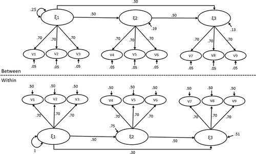
where μ_j has the cluster means of the indicators in cluster j, ξ_j contains the cluster-level factor scores for cluster j, ε_j contains the residual factor scores for cluster j, and Λ contains the factor loadings. The factor scores ξ_j are drawn from a multivariate normal distribution with zero means and covariance matrix Φ_BETWEEN:

(4) ${\mathbf{\Phi }}_{\mathrm{B}\mathrm{E}\mathrm{T}\mathrm{W}\mathrm{E}\mathrm{E}\mathrm{N}}={\left(\mathbf{I}\mathbf{-}{\mathbf{B}}_{\mathrm{B}\mathrm{E}\mathrm{T}\mathrm{W}\mathrm{E}\mathrm{E}\mathrm{N}}\right)}^{-1}{\mathbf{\Psi }}_{\mathrm{B}\mathrm{E}\mathrm{T}\mathrm{W}\mathrm{E}\mathrm{E}\mathrm{N}}{\left(\mathbf{I}\mathbf{-}{\mathbf{B}}_{\mathrm{B}\mathrm{E}\mathrm{T}\mathrm{W}\mathrm{E}\mathrm{E}\mathrm{N}}\right)}^{-1\mathrm{T}}$(4)

where Β_BETWEEN is a square matrix with regression coefficients between the common factors, Ψ_BETWEEN is a symmetric matrix with the variances and covariances at the between-level, and I is an identity matrix with the same dimensions as Β_BETWEEN. Residual factor scores ε_j are also drawn from a multivariate normal distribution with zero means and a diagonal covariance matrix. In the next step, we drew data from the multivariate normal distribution for each cluster, with means corresponding to the associated cluster means μ_j from the previous step, and covariance matrix Σ_WITHIN:

(5) ${\mathbf{\Sigma }}_{\mathrm{W}\mathrm{I}\mathrm{T}\mathrm{H}\mathrm{I}\mathrm{N}}=\mathbf{\Lambda }{\mathbf{\Phi }}_{\mathrm{W}\mathrm{I}\mathrm{T}\mathrm{H}\mathrm{I}\mathrm{N}}{\mathbf{\Lambda }}^{\mathrm{T}}+{\mathbf{\Theta }}_{\mathrm{W}\mathrm{I}\mathrm{T}\mathrm{H}\mathrm{I}\mathrm{N}}$(5)

Figure 2 shows the population values for all parameters in the conditions with an intraclass correlation (ICC) of .15. In the ICC = .05 conditions, the variances at the between-level were smaller than in the ICC = .15 conditions. To create ICCs of .05, the residual variance at the between-level was .01, the variance of the exogenous factor at the between-level was 0.09, and the residual variance of the mediating factor and outcome factor were 0.0675 and 0.0459, respectively, leading to total factor variances of .09. Note that the mentioned ICC-values refer to the intraclass correlations of the observed variables. The ICC of the common factors in the ICC = .15 condition are .25/(1 + .25) = .20, while in the ICC = .05 conditions they are .09/(1 + .09) = .08. The R-code used for data generation and analysis is available through this link: https://www.dropbox.com/s/pixhqqt8pauxckl/sim_multilevel_mediation3.R?dl=0.

Conditions

We varied the ICC-values (ICC = .15 or CC = .05), the number of clusters (20, 40, 80, or 100), and the cluster size (5, 20, 40, 60, 1000), leading to 40 conditions. These conditions include all sample size conditions that were evaluated by Li and Beretvas (2013), and in addition evaluate cluster sizes of 1000 that are representative of cross-cultural datasets such as PISA (OECD, 2016) and the European Social Survey (ESS, 2016), and cluster sizes of 5 that are encountered in educational research (Zee, Koomen, Jellesma, Geerlings, & de Jong, 2016) and organizational research (Jackson & Joshi, 2004). We also evaluated conditions with 100 clusters, which was found to be the minimum acceptable cluster size for which the chi-square statistic follows its expected asymptotic distribution to reasonable approximation (Hox et al., 2010). We generate 2000 datasets per condition.

Evaluation criteria and expectations

To each dataset, we fitted the correctly specified model with equality constraints on the factor loadings, and the same model without the equality constraints. We will refer to these models as the “invariance model” and the “free model,” respectively. We used lavaan version 0.6–3 (Rosseel, 2012), which provides maximum likelihood estimation and robust standard errors (Huber, 1967; White, 1982) for all model parameters.

Evaluation criteria were convergence rates, the proportion of replications that resulted in a warning message, the proportion of replications that resulted in negative variance estimates at the between-level, and true positive rates of the Wald-test on the direct and indirect effects. These evaluation criteria were selected because these are outcomes that are expected to be different across the free and invariant model. While convergence rates and true positive rates are common outcomes in simulation studies, we are not aware of other studies that evaluate the frequency of warning messages or negative variance estimates. Typical warning messages that one obtains when analyzing MLSEM are messages about negative between-level variances and problems with convergence or obtaining standard errors. These error messages are of course informative, but in practice often lead researchers to doubt whether the results can be trusted, potentially leading to rejection of the model. In the evaluation of the results we do not differentiate between different types of warnings, but we will evaluate the actual convergence rates and frequencies of negative variance estimates.

True positive rates of the direct effect of Factor 1 on Factor 3 (β₃₁ in Figure 2) and the indirect effect (β₂₁ * β₃₂ in Figure 2) are evaluated by calculating the proportion of replications for which the ratio of the parameter estimate over the associated standard error was larger than 1.96. Given the asymmetry of the sampling distribution of indirect effects, bootstrapping methods are to be preferred over the simple z-test in practice (MacKinnon, Lockwood, & Williams, 2004). Still, we apply the z-test here because using bootstrapping methods would make execution of the simulation study extremely slow, and the differences in true positive rates between the invariant and free model will be similar across methods.

Because the free model is overparameterized, we expect that the free model leads to larger numbers of non-converged replications, more negative variance estimates at the between-level, and to more error messages (Bates, Kliegl, Vasishth & Baayen, 2015). We also expect that the true positive rates for the direct and indirect effects will be larger for the invariant model than for the free model.

RESULTS

We present all results graphically, in order to display the patterns in the results across conditions. The exact numerical results, as well as significance tests comparing the results for the free and invariant models, for all outcomes in all conditions can be found in Tables A1, A2, and A3 in Appendix A.

Convergence

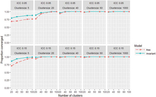
Figure 3 shows the convergence rates for the free and invariant model in all conditions. As expected, the invariant model leads to better or similar convergence rates than the free model in all conditions. With at least 40 observations per cluster, convergence is no problem for both models. For cluster sizes of 5, the proportion of converged solutions in the smallest sample size conditions was as low as 0.68–0.72 for the free model, and 0.80–0.87 for the invariant model. Convergence rates increased with larger numbers of clusters. For the remainder of the results section we only evaluated replications for which both the free and the invariance model converged.

FIGURE 3 Convergence rates for the free and invariant model in all conditions.

Warnings

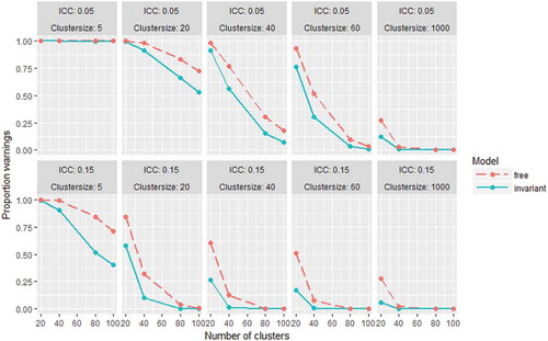
Figure 4 shows the proportions of replications that issued a warning per condition. As expected, the free model led to more (or equal) solutions with warnings than the invariant model. Overall, less warnings are observed with increasing cluster sizes, with increasing number of clusters, and with larger ICC. In the ICC = .05 conditions (upper panel of Figure 4), all datasets with cluster sizes of 5 produced warnings for both models. Both models produce less than 5% warnings only with at least 40 clusters of size 1000, and for the invariant model also with at least 80 clusters of size 60 or larger. In the ICC = .15 conditions (see lower panel of Figure 4), both models lead to less than 5% warnings with at least 80 clusters of size 50 or larger, and with at least 40 clusters of size 1000. The invariant model in addition leads to less than 5% warnings with at least 40 clusters of size 40, and with 20 clusters of 1000.

FIGURE 4 Proportions of replications with warnings for the free and invariant model in all conditions.

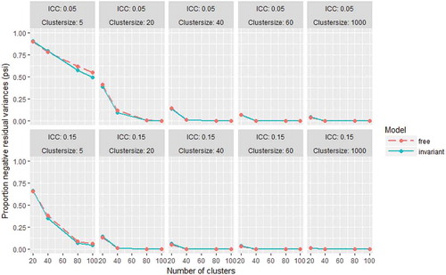
Negative residual variances

Figures 5 and 6 respectively show the proportions of replications that resulted in a negative residual variance estimate for an observed variable (in Θ) and a latent variable (in Ψ) at the between-level. The differences between the free and invariant model in the occurrence of negative variances for latent variables were negligible in almost all conditions, and high proportions of negative estimates were only found in the smalles sample size conditions. The frequency of negative estimates of the residual variances of the observed variables was larger for the free model than for the invariant model in most conditions, and similar in some conditions. For both models, the proportions decreased with increasing number of clusters, cluster size, and ICC. In the ICC = 0.05 conditions, both models lead to negative variance estimates in practically all replications with cluster sizes of 5. Less than 5% negative variance estimates was obtained for both models with at least 40 clusters of size 1000, and for the invariant model already with 80 clusters of at least size 60. In the ICC = 0.15 conditions, less than 5% negative variance estimates was found for both model with at least 80 clusters with cluster sizes 20 or larger, and for the invariant model also with at least 40 clusters of size 40, or at least 20 clusters of size 1000.

FIGURE 5 Proportions of replications with negative residual variance estimates for observed variables at the between-level (θ_B) for the free and invariant model in all conditions.

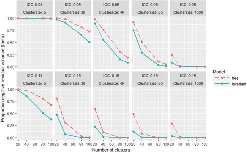
FIGURE 6 Proportions of replications with negative residual variance estimates for latent variables at the between-level for the free and invariant model in all conditions.

True positive rates

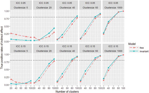
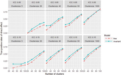
True positive rates of the direct effect were larger for the invariant model than for the free model in all conditions (see Figure 7). As may be expected, the true positive rates increase with larger number of clusters of larger cluster sizes. Overall the true positive rates are higher in the ICC = 0.05 condition than in the ICC = .15 condition. For the direct effect, true positive rates are higher than .80 only in ICC = .05 conditions with at least 100 clusters with size 1000. In the ICC = .15 conditions, only the invariant model leads to true positive rates higher than .80, in conditions with at least 100 clusters of 1000. An explanation for the higher true positive rates in the smaller ICC-condition is that there was relatively more residual variance present in ICC = .15 conditions. In the ICC = .05 condition, the percentage of residual variance at the between-level was .01/(.70²*.09 + .01) * 100% = 18.4%, while in the ICC = .15 conditions this percentage was .05/(.70²*.25 + .05) * 100% = 29.0%. More residual variance at the between-level negatively affects the true positive rates on test of direct effects between common factors.

FIGURE 7 True positive rates of the direct effect (β₃₁) for the free and invariant model in all conditions. The dashed horizontal line marks a true positive rate of 0.80.

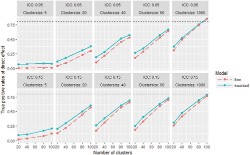
The results shown here are based on all converged replications, including the replications that lead to a warning. In Appendix B, we show the results for only the replications for which both models converged without warnings. In small sample conditions all replications lead to warnings, so there were no results left to analyze, but in the other conditions the true positive rates are practically identical to those in Figure 7.

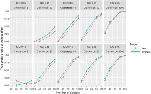
Since the z-test is not recommended for testing the significance of indirect effects in practice, we do not discuss the absolute values of true positive rates for the indirect effect. Still, it is informative to see that the true positive rates are higher for the invariant model in almost all conditions (Figure 8). Contrary to expectations, in the conditions with cluster sizes of 5, the free model had larger true positive rates than the invariant model, and the true positive rates tend to decrease with increasing number clusters. These results are hard to interpret, and show that the behavior of the z-test for indirect effects may be erratic at small sample size conditions.

FIGURE 8 True positive rates of the indirect effect (β₂₁ * β₃₂) for the free and invariant model in all conditions. The dashed horizontal line marks a true positive rate of 0.80.

DISCUSSION

This simulation study showed that, in addition to the theoretical need for cross-level invariance in multilevel factor models (Asparouhov & Muthen, 2012; Hox et al., 2017; Jak et al., 2013; Kim et al., 2016; Mehta & Neale, 2005; Muthén, 1990; Rabe-Hesketh et al., 2004; Stapleton et al., 2016), constraining factor loadings across levels decreases estimation problems and increases true positive rates. Not applying cross-level invariance constraints when factor loadings are equal in the population leads to models that are too complex for the data, which increases estimation problems and decreases the power to detect true effects. Thus, researchers who plan to fit factor models to multilevel data should carefully think about the theoretical meaning of the factor(s) at the different levels. If a common factor at the higher level is to be interpreted as the between component of the factor at the lower level, cross-level invariance should be applied. In the remainder of the discussion, we will discuss some directions for future research on cross-level invariance in MLSEM.

If cross-level invariance does not hold

If in the population the factor loadings are unequal, then the model with cross-level invariance constraints is misspecified. It can be expected that this will lead to biased parameter estimates, biased standard errors, and bad coverage rates for confidence intervals. Indeed, Guenole (2016) found that inappropriately applying these constraints leads to untrustworthy results in the Bayesian framework with ordinal indicators. However, Guenole evaluated conditions with relatively large differences between the factor loadings at the two levels, because the population values of factor loadings in his study were based on standardized factor loadings, leading to much higher factor loadings at the between-level than at the within-level (Jak & Jorgensen, 2017). Kim et al, in another simulation study, found that applying cross-level invariance in conditions where factor loadings where actually not equal across levels lead to better performance of testing latent group mean difference across within-level groups. These contrasting results suggest that there may be a point where the benefits of applying cross-level invariance constraints on estimation performance outweighs the detrimental effects it has when the constraint is actually not appropriate. Future research may focus on the effect of applying cross-level invariance in conditions where there are smaller differences between loadings at different levels, and in conditions where only part of the loadings are invariant.

If cross-level invariance doesn’t hold, the associated factors do not have the same interpretation across levels. For example, if the factor loading for a specific indicator is higher at the between-level than at the within-level, than the factor at the between-level will represent more of the content of that specific indicator (and the other way around). In research about the closeness of teacher-student relations for example, an item about whether a student “openly shares feelings” was found to be more indicative at the student level than at the teacher level (Spilt, Koomen, & Jak, 2012). By freeing the invariance constraint on this factor loading, the interpretation of the common factor at the student level includes more of the attribute “openly sharing feelings” than the factor at the teacher level. One can imagine that if several factor loadings differ in several directions across levels, it will become complicated to pinpoint how to interpret the factors exactly. Although the interpretation of factors will become difficult if cross-level invariance does not apply, in specific situations it may still be interesting to evaluate how the factor loadings differ across levels. Tay, Woo, and Vermunt (2014) provide a discussion of weaker forms of cross-level invariance, such as cases where not the exact values, but the rank order of the size of factor loadings is the same across levels.

Cross-level invariance for shared constructs

Stapleton et al. discussed several possible multilevel factor models based on individual-level measures. In their taxonomy, configural construct models represent those models in which the common factor of interest features both at the within- and between-level, and the authors explained that cross-level invariance constraints are needed for these models. Another type of constructs that they discuss are shared constructs, where the construct represents a characteristic of the cluster, and the within-level construct is not of direct interest. For example, researchers could be interested in measuring teacher quality, using the evaluations of the teacher’s students. For a truly shared construct, the item responses from students within the same classroom can be seen as interchangeable (Bliese, 2000). That is, the responses across students within the same classroom would be perfectly correlated at the population level, and all differences in responses within classrooms represent random variation. The model at the within-level is not interesting in this situation, leading Stapleton at al. to propose fitting a saturated model at the within-level. However, this situation can also be represented using the same model as for configural constructs. One could apply a two-level factor model (with cross-level invariance) to these data, such that the common factor model at the between-level represents the between component of teacher quality, and the factor at the within-level represents the within component of teacher quality. For truly shared constructs, however, the within-component of teacher quality does not exist; there are assumed to be no structural differences in the student’s evaluation of teacher quality. Absence of these differences would imply zero covariance between the items at the within-level, and hence zero variance for the common factor at the within-level. The random variation at the student-level would then be represented by the residual variance at the within-level. The configural model specification would thus represent the situation for shared constructs as well, by allowing the factor variance at the within-level to be zero. This configuration leads to less parameters than the saturated model. For example, with 5 indicators and 1 common factor, the saturated model would lead to 5 * (6)/2 = 15 parameters to be estimated, while the configural model would lead to 5 (residual variances) + 1 (factor variance) = 6 parameters to be estimated. The saturated model is thus effectively overparameterized in this situation, potentially leading to estimation problems. Another advantage of using the factor model with cross-level invariance for theoretically shared constructs, is that if the construct is not truly shared, such that differences in individuals’ responses do reflect differences in the individuals’ evaluation of the between-level construct of interest, then this would be easily captured by non-zero factor variance at the within-level. Future research may evaluate the performance of this model for shared constructs.

Other suggestions for future research

The current simulation study only evaluated conditions in which the model was correctly specified, and mainly focused on estimation problems as outcomes. This gives a clear picture of what may be expected if theoretically configural factors are not modelled as such. However, as is often the case with simulation studies, it is not difficult to think of other conditions and outcomes that would be interesting to investigate. For example, it could be interesting to evaluate conditions where cross-level invariance does not hold, and to evaluate model fit statistics under different conditions. Such a study would be informative to show whether for example the likelihood ratio test is able to detect the non-invariance in factor loadings, and how large the non-invariance should be to lead to biased results. The current simulation study was also limited to the evaluation of one specific multilevel mediation model, and by using one specific software package (lavaan 0.6–3). One can imagine that other SEM-programs, such as xxM (Mehta, 2013) or Mplus (Muthén & Muthén, 1998-2017), have slightly different implementations leading to different results with regard to convergence and warnings. Future research may evaluate these other conditions, outcomes, and other software packages.

Additional information

Funding

This work was supported by the Netherlands Organization for Scientific Research [NWO-VENI-451-16-001].

Appendix A:

Tables containing all results

Table A1 Proportions of Replications with Convergence Issues and Warnings

			Convergence			Warnings
ICC	NB	CS	FREE	INV	Δ sign	FREE	INV	Δ sign
0.05	20	5	0.676	0.804	YES	1.000	1.000	NO
		20	0.818	0.893	YES	0.999	0.991	NO
		40	0.943	0.968	YES	0.985	0.919	YES
		60	0.986	0.992	NO	0.930	0.772	YES
		1000	0.990	0.988	NO	0.288	0.124	YES
	40	5	0.710	0.832	YES	1.000	0.999	NO
		20	0.938	0.973	YES	0.985	0.924	YES
		40	0.996	0.997	NO	0.769	0.562	YES
		60	1.000	1.000	NO	0.515	0.300	YES
		1000	0.998	1.000	NO	0.018	0.007	NO
	80	5	0.743	0.877	YES	1.000	0.997	NO
		20	0.996	0.998	NO	0.821	0.656	YES
		40	1.000	1.000	NO	0.316	0.159	YES
		60	1.000	1.000	NO	0.108	0.032	YES
		1000	1000	1.000	NO	0.000	0.000	NO
	100	5	0.774	0.899	YES	0.999	0.996	NO
		20	0.998	0.999	NO	0.719	0.509	YES
		40	1.000	1.000	NO	0.196	0.082	YES
		60	1.000	1.000	NO	0.046	0.013	YES
		1000	1.000	1.000	NO	0.000	0.000	NO
0.15	20	5	0.716	0.870	YES	1.000	0.994	NO
		20	0.934	0.978	YES	0.838	0.561	YES
		40	0.978	0.994	YES	0.624	0.274	YES
		60	0.988	0.998	YES	0.511	0.161	YES
		1000	0.999	0.998	NO	0.301	0.050	YES
	40	5	0.793	0.929	YES	0.987	0.924	YES
		20	0.996	1.000	NO	0.320	0.084	YES
		40	1.000	1.000	NO	0.116	0.021	YES
		60	1.000	1.000	NO	0.083	0.006	YES
		1000	1.000	1.000	NO	0.013	0.000	NO
	80	5	0.938	0.984	YES	0.826	0.554	YES
		20	1.000	1.000	NO	0.032	0.002	YES
		40	1.000	1.000	NO	0.004	0.000	NO
		60	1.000	1.000	NO	0.002	0.000	NO
		1000	1.000	1.000	NO	0.000	0.000	NO
	100	5	0.972	0.991	YES	0.693	0.412	YES
		20	1.000	1.000	NO	0.010	0.000	YES
		40	1.000	1.000	NO	0.001	0.000	NO
		60	1.000	1.000	NO	0.000	0.000	NO
		1000	1.000	1.000	NO	0.000	0.000	NO

Note. ICC = intraclass correlation, NB = number of clusters, CS = cluster size, FREE = model with unconstrained factor loadings, INV = model with constrained factor loadings across levels, Δ sign = YES/NO indicates if the rates differ across the FREE and INV model as tested with McNemar’s test for dependent proportions with α = 0.05/(40 conditions*6 outcomes). Warnings are based on converged replications only.

Table A2 Proportions of Replications with Negative Residual Variances at the Between-Level

			Negative estimate in ΘBETWEEN			Negative estimate in ΨBETWEEN
ICC	NB	CS	FREE	INV	Δ sign	FREE	INV	Δ sign
0.05	20	5	1.000	1.000	NO	0.902	0.908	NO
		20	0.999	0.977	YES	0.415	0.388	NO
		40	0.979	0.897	YES	0.145	0.141	NO
		60	0.921	0.750	YES	0.071	0.073	NO
		1000	0.253	0.082	YES	0.038	0.043	NO
	40	5	0.997	0.994	NO	0.785	0.794	NO
		20	0.979	0.914	YES	0.121	0.093	YES
		40	0.761	0.554	YES	0.014	0.013	NO
		60	0.514	0.298	YES	0.001	0.001	NO
		1000	0.015	0.003	YES	0.004	0.005	NO
	80	5	0.998	0.992	NO	0.622	0.577	NO
		20	0.817	0.651	YES	0.011	0.007	NO
		40	0.316	0.159	YES	0.000	0.000	NO
		60	0.108	0.032	YES	0.000	0.000	NO
		1000	0.000	0.000	NO	0.000	0.000	NO
	100	5	0.998	0.990	NO	0.549	0.498	YES
		20	0.718	0.507	YES	0.003	0.002	NO
		40	0.196	0.082	YES	0.000	0.000	NO
		60	0.046	0.013	YES	0.000	0.000	NO
		1000	0.000	0.000	NO	0.000	0.000	NO
0.15	20	5	0.998	0.967	YES	0.656	0.664	NO
		20	0.799	0.473	YES	0.131	0.147	NO
		40	0.597	0.224	YES	0.051	0.062	NO
		60	0.487	0.125	YES	0.032	0.041	NO
		1000	0.290	0.035	YES	0.014	0.017	NO
	40	5	0.967	0.848	YES	0.379	0.350	NO
		20	0.308	0.073	YES	0.015	0.012	NO
		40	0.114	0.020	YES	0.002	0.002	NO
		60	0.082	0.005	YES	0.001	0.002	NO
		1000	0.013	0.000	NO	0.000	0.000	NO
	80	5	0.802	0.511	YES	0.090	0.070	NO
		20	0.031	0.002	YES	0.000	0.000	NO
		40	0.004	0.000	NO	0.000	0.000	NO
		60	0.002	0.000	NO	0.000	0.000	NO
		1000	0.000	0.000	NO	0.000	0.000	NO
	100	5	0.670	0.381	YES	0.063	0.042	YES
		20	0.010	0.000	YES	0.000	0.000	NO
		40	0.001	0.000	NO	0.000	0.000	NO
		60	0.000	0.000	NO	0.000	0.000	NO
		1000	0.000	0.000	NO	0.000	0.000	NO

Note. ICC = intraclass correlation, NB = number of clusters, CS = cluster size, FREE = model with unconstrained factor loadings, INV = model with constrained factor loadings across levels, Δ sign = YES/NO indicates if the rates differ across the FREE and INV model as tested with McNemar’s test for dependent proportions with α = 0.05/(40 conditions*6 outcomes). Results are based on converged replications only.

Table A3 Proportions of Replications with Significant Direct and Indirect Effects

			TP direct effect			TP indirect effect
ICC	NB	CS	FREE	INV	Δ sign	FREE	INV	Δ sign
0.05	20	5	0.007	0.085	YES	0.270	0.089	YES
		20	0.048	0.141	YES	0.130	0.032	YES
		40	0.120	0.188	YES	0.071	0.066	NO
		60	0.169	0.242	YES	0.069	0.098	YES
		1000	0.305	0.357	YES	0.230	0.283	YES
	40	5	0.011	0.085	YES	0.209	0.070	YES
		20	0.099	0.197	YES	0.052	0.056	NO
		40	0.215	0.274	YES	0.142	0.226	YES
		60	0.302	0.363	YES	0.263	0.344	YES
		1000	0.493	0.527	YES	0.584	0.631	YES
	80	5	0.013	0.072	YES	0.161	0.038	YES
		20	0.225	0.324	YES	0.157	0.259	YES
		40	0.447	0.496	YES	0.558	0.664	YES
		60	0.536	0.566	YES	0.742	0.794	YES
		1000	0.770	0.777	NO	0.964	0.968	NO
	100	5	0.015	0.087	YES	0.116	0.033	YES
		20	0.307	0.394	YES	0.273	0.418	YES
		40	0.545	0.599	YES	0.736	0.818	YES
		60	0.629	0.657	YES	0.884	0.916	YES
		1000	0.832	0.840	NO	0.990	0.992	NO
0.15	20	5	0.017	0.095	YES	0.172	0.040	YES
		20	0.137	0.214	YES	0.067	0.062	NO
		40	0.181	0.264	YES	0.079	0.118	YES
		60	0.205	0.273	YES	0.092	0.141	YES
		1000	0.243	0.313	YES	0.155	0.215	YES
	40	5	0.029	0.117	YES	0.095	0.025	YES
		20	0.226	0.304	YES	0.144	0.234	YES
		40	0.306	0.366	YES	0.256	0.348	YES
		60	0.342	0.391	YES	0.312	0.422	YES
		1000	0.398	0.452	YES	0.456	0.556	YES
	80	5	0.099	0.188	YES	0.036	0.059	YES
		20	0.434	0.498	YES	0.592	0.690	YES
		40	0.537	0.578	YES	0.776	0.834	YES
		60	0.588	0.624	YES	0.838	0.882	YES
		1000	0.658	0.686	YES	0.918	0.946	YES
	100	5	0.104	0.209	YES	0.065	0.123	YES
		20	0.540	0.584	YES	0.755	0.824	YES
		40	0.669	0.694	YES	0.906	0.934	YES
		60	0.690	0.712	YES	0.939	0.960	YES
		1000	0.781	0.802	YES	0.980	0.984	NO

Note. ICC = intraclass correlation, NB = number of clusters, CS = cluster size, TP = yes positive rate, FREE = model with unconstrained factor loadings, INV = model with constrained factor loadings across levels, Δ sign = YES/NO indicates if the rates differ across the FREE and INV model as tested with McNemar’s test for dependent proportions with α = 0.05/(40 conditions*6 outcomes). Results are based on converged replications only. Cells from conditions that show results in the unexpected direction are marked italic (mainly CS = 5 conditions)

Appendix B:

True positive rates from only the replications without warnings

True positive rates of direct effect

True positive rates of the indirect effect

References

- Asparouhov, T., & Muthen, B. (2012). Multiple group multilevel analysis (mplus web notes no. 16). Retrieved from http://statmodel.com/examples/webnotes/webnote16.pdf
- Bates, D., Kliegl, R., Vasishth, S., & Baayen, R. H. (2015). Parsimonious mixed models. arXiv:1506.04967 (stat.ME).
- Bliese, P. (2000). Within-group agreement, non-independence, and reliability: Implications for data aggregation and analysis. In K. J. Klein & S. W. J. Kozlowski (Eds.), Multilevel theory, research, and methods in organizations: Foundations, extensions, and new directions (pp. 349–381). San Francisco, CA: Jossey-Bass.
- De Jong, M. G., Steenkamp, J. B. E. M., & Fox, J.-P. (2007). Relaxing measurement invariance in cross-national consumer research using a hierarchical IRT model. Journal of Consumer Research, 34, 260–278. doi:10.1086/518532
- Depaoli, S., & Clifton, J. P. (2015). A Bayesian approach to multilevel structural equation modeling with continuous and dichotomous outcomes. Structural Equation Modeling, 22, 327–351. doi:10.1080/10705511.2014.937849
- European Social Survey. (2016). ESS 1-7, European social survey cumulative file, study description. Bergen, Norway: NSD - Norwegian Centre for Research Data for ESS ERIC.
- González-Romá, V., & Hernández, A. (2017). Multilevel modeling: Research-based lessons for substantive researchers. Annual Review of Organizational Psychology and Organizational Behavior, 4, 183–210. doi:10.1146/annurev-orgpsych-041015-062407
- Guenole, N. (2016). The importance of isomorphism for conclusions about homology: A Bayesian multilevel structural equation modeling approach with ordinal indicators. Frontiers in Psychology, 7, 289. doi:10.3389/fpsyg.2016.00289
- Holtmann, J., Koch, T., Lochner, K., & Eid, M. (2016). A comparison of ML, WLSMV, and Bayesian methods for multilevel structural equation models in small samples: A simulation study. Multivariate Behavioral Research, 51, 661–680. doi:10.1080/00273171.2016.1208074
- Hox, J. J., Maas, C. J. M., & Brinkhuis, M. J. S. (2010). The effect of estimation method and sample size in multilevel structural equation modeling. Statistica Neerlandica, 64, 157–170. doi:10.1111/j.1467-9574.2009.00445.x
- Hox, J. J., Moerbeek, M., & van de Schoot, R. (2017). Multilevel analysis: Techniques and applications. New York, NY: Routledge.
- Huber, P. J. (1967). The behavior of maximum likelihood estimates under non-standard conditions. In: Proceedings of the Fifth Berkeley Symposium on Mathematical Statistics and Probability, pp. (221–233). Berkeley: University of California Press.
- Jackson, S. E., & Joshi, A. (2004). Diversity in social context: A multi-attribute, multilevel analysis of team diversity and sales performance. Journal of Organizational Behavior, 25, 675–702. doi:10.1002/job.265
- Jak, S., & Jorgensen, T. D. (2017). Relating measurement invariance, cross-level invariance, and multilevel reliability. Frontiers in Psychology, 8, 1640. doi:10.3389/fpsyg.2017.01640
- Jak, S., Oort, F. J., & Dolan, C. V. (2013). A test for cluster bias: Detecting violations of measurement invariance across clusters in multilevel data. Structural Equation Modeling, 20, 265–282. doi:10.1080/10705511.2013.769392
- Jak, S., Oort, F. J., & Dolan, C. V. (2014). Using two-level factor analysis to test for cluster bias in ordinal data. Multivariate Behavioral Research, 49, 544–553. doi:10.1080/00273171.2014.947353
- Kim, E. S., & Cao, C. (2015). Testing group mean differences of latent variables in multilevel data using multiple-group multilevel CFA and multilevel MIMIC modeling. Multivariate Behavioral Research, 50, 436–456. doi:10.1080/00273171.2015.1021447
- Kim, E. S., Dedrick, R. F., Cao, C., & Ferron, J. M. (2016). Multilevel factor analysis: Reporting guidelines and a review of reporting practices. Multivariate Behavioral Research, 51, 881–898. doi:10.1080/00273171.2016.1228042
- Kim, E. S., Yoon, M., Wen, Y., Luo, W., & Kwok, O. M. (2015). Within-level group factorial invariance with multilevel data: Multilevel factor mixture and multilevel MIMIC models. Structural Equation Modeling, 22, 603–616. doi:10.1080/10705511.2014.938217
- Lee, W. Y., & Cho, S. J. (2017). Detecting Differential Item Discrimination (DID) and the consequences of ignoring DID in multilevel item response models. Journal of Educational Measurement, 54(3), 364–393. doi:10.1111/jedm.12148
- Li, X., & Beretvas, S. N. (2013). Sample size limits for estimating upper level mediation models using multilevel SEM. Structural Equation Modeling, 20(2), 241–264. doi:10.1080/10705511.2013.769391
- Lüdtke, O., Marsh, H. W., Robitzsch, A., & Trautwein, U. (2011). A 2 × 2 taxonomy of multilevel latent contextual models: Accuracy–Bias trade-offs in full and partial error correction models. Psychological Methods, 16, 444–467. doi:10.1037/a0024376
- MacKinnon, D. P., Lockwood, C. M., & Williams, J. (2004). Confidence limits for the indirect effect: Distribution of the product and resampling methods. Multivariate Behavioral Research, 39(1), 99–128. doi:10.1207/s15327906mbr3901_4
- Marsh, H. W., Lüdtke, O., Robitzsch, A., Trautwein, U., Asparouhov, T., Muthén, B., & Nagengast, B. (2009). Doubly-latent models of school contextual effects: Integrating multilevel and structural equation approaches to control measurement and sampling error. Multivariate Behavioral Research, 44(6), 764–802. doi:10.1080/00273170903333665
- Mehta, P. D. (2013). xxM User’s guide. [Online document]. Retrieved from http://xxm.times.uh.edu/documentation/xxm.pdf
- Mehta, P. D., & Neale, M. C. (2005). People are variables too: Multilevel structural equations modeling. Psychological Methods, 10, 259–284. doi:10.1037/1082-989X.10.3.259
- Muthén, B. (1990). Mean and covariance structure analysis of hierarchical data. Los Angeles, CA: UCLA.
- Muthén, B. O. (1989). Latent variable modeling in heterogeneous populations. Psychometrika, 54(4), 557–585. doi:10.1007/BF02296397
- Muthén, B. O. (1994). Multilevel covariance structure analysis. Sociological Methods & Research, 22, 376–398. doi:10.1177/0049124194022003006
- Muthén, L. K., & Muthén, B. O. (1998/2017). Mplus User’s guide. (8thed.). Los Angeles, CA: Muthén & Muthén.
- OECD. (2016). PISA 2015 results (Volume I): Excellence and equity in education. Paris, France: Author. doi:10.1787/9789264266490-en
- Preacher, K. J., Zyphur, M. J., & Zhang, Z. (2010). A general multilevel SEM framework for multilevel mediation. Psychological Methods, 15, 209–233. doi:10.1037/a0020141
- R Core Team. (2018). R: A language and environment for statistical computing. Vienna, Austria: R Foundation for Statistical Computing. Retrieved from https://www.R-project.org/
- Rabe-Hesketh, S., Skrondal, A., & Pickles, A. (2004). Generalized multilevel structural equation modelling. Psychometrika, 69, 167–190. doi:10.1007/BF02295939
- Rosseel, Y. (2012). lavaan: An R package for structural equation modeling. Journal of Statistical Software, 48(2), 1–36. doi:10.18637/jss.v048.i02
- Schmidt, W. H. (1969). Covariance structure analysis of the multivariate random effects model ( Doctoral dissertation, University of Chicago, Department of Education).
- Spilt, J. L., Koomen, H. M., & Jak, S. (2012). Are boys better off with male and girls with female teachers? A multilevel investigation of measurement invariance and gender match in teacher–Student relationship quality. Journal of School Psychology, 50(3), 363–378. doi:10.1016/j.jsp.2011.12.002
- Stapleton, L. M., Yang, J. S., & Hancock, G. R. (2016). Construct meaning in multilevel settings. Journal of Educational and Behavioral Statistics, 41(5), 481–520. doi:10.3102/1076998616646200
- Tay, L., Woo, S. E., & Vermunt, J. K. (2014). A conceptual framework of cross-level isomorphism: Psychometric validation of multilevel constructs. Organizational Research Methods, 17, 77–106. doi:10.1177/1094428113517008
- Venables, W. N., & Ripley, B. D. (2002). Modern Applied Statistics with S (4th ed.). New York, NY: Springer.
- White, H. (1982). Maximum likelihood estimation of misspecified models. Econometrica, 50, 1–25. doi:10.2307/1912526
- Zee, M., Koomen, H. M., Jellesma, F. C., Geerlings, J., & de Jong, P. F. (2016). Inter-and intra-individual differences in teachers’ self-efficacy: A multilevel factor exploration. Journal of School Psychology, 55, 39–56. doi:10.1016/j.jsp.2015.12.003