Latent Markov Factor Analysis for Exploring Measurement Model Changes in Time-Intensive Longitudinal Studies

Abstract

When time-intensive longitudinal data are used to study daily-life dynamics of psychological constructs (e.g., well-being) within persons over time (e.g., by means of experience sampling methodology), the measurement model (MM)—indicating which constructs are measured by which items—can be affected by time- or situation-specific artifacts (e.g., response styles and altered item interpretation). If not captured, these changes might lead to invalid inferences about the constructs. Existing methodology can only test for a priori hypotheses on MM changes, which are often absent or incomplete. Therefore, we present the exploratory method “latent Markov factor analysis” (LMFA), wherein a latent Markov chain captures MM changes by clustering observations per subject into a few states. Specifically, each state gathers validly comparable observations, and state-specific factor analyses reveal what the MMs look like. LMFA performs well in recovering parameters under a wide range of simulated conditions, and its empirical value is illustrated with an example.

Keywords:

• experience sampling
• measurement invariance
• factor analysis
• latent Markov modeling

Introduction

Time-intensive longitudinal data for studying daily-life dynamics of psychological constructs (such as well-being and positive affect) within persons allow to delve into time- or situation-specific effects (e.g., stress) on the (e.g., emotional) experiences of a large number of subjects (Larson & Csikszentmihalyi, 2014). The go-to research design to collect such data is experience sampling methodology (ESM; Scollon, Kim-Prieto, & Diener, 2003). Participants repeatedly answer questionnaires at randomized or event-based time-points via smartphone apps, for example, eight times a day over a few weeks.

While the technology for collecting ESM data is readily available, the methodology to validly analyze these data are lagging behind. This article provides an upgrade of the methodology by presenting a novel method for tracking and diagnosing changes in measurement models (MMs) over time. The MM is the model underlying a participant’s answers and indicates which unobservable or latent variables (i.e., psychological constructs) are measured by which items. Traditionally, it is evaluated by factor analysis (FA; Lawley & Maxwell, 1962), where the factors correspond—ideally—to the hypothesized constructs. Factor loadings express the degree to which each of the items measures a factor and thus how strongly an item relates to an underlying factor. In order to meaningfully compare constructs over time, the MM needs to be invariant across measurement occasions (Adolf, Schuurman, Borkenau, Borsboom, & Dolan, 2014). However, measurement invariance (MI) does not always hold over time because the MM likely changes over the course of an ESM study. First, in ESM, the measurement quality is undermined by time- or situation-specific artifacts such as response styles (RSs; Moors, 2003; Paulhus, 1991). Indeed, participants fill in their questionnaires repeatedly in various, possibly distracting, situations (e.g., during work) or lose motivation to repeatedly answer questions, which may drive the tendency to, for example, use the extreme response categories only (extreme RS; Moors, 2003; Morren, Gelissen, & Vermunt, 2011). Second, substantive changes may occur over time in what questionnaire items are measuring. For example, depending on the context or mental state, an item may become more important for the measured construct (i.e., loading increases) or (also) an indicator of another construct (i.e., loads strongly on another factor; reprioritization or reconceptualization; Oort, Visser, & Sprangers, 2005). Moreover, the nature of the measured constructs might change entirely; for example, when positive affect and negative affect factors are replaced by high and low arousal factors (Feldman, 1995). In any case, when ignoring changes in the MM, changes in the scores will be interpreted as changes in the psychological constructs, although they are (partly) caused by RSs or changed item interpretation.

To safeguard validity of their time-intensive longitudinal studies, substantive researchers need an efficient approach to evaluate which MMs are underlying the data and for which time-points they apply, so that they can gain insight into which artifacts and substantive changes are at play and when. Researchers can take these insights into account when analyzing the data, when setting up future projects or to derive new substantive findings from the MM changes. To meet this need, we present latent Markov factor analysis (LMFA),¹ which combines two building blocks to model MM changes within subjects over time: (1) latent Markov modeling (LMM; Bartolucci, Farcomeni, & Pennoni, 2014; Collins & Lanza, 2010) clusters time-points into states according to the MMs and (2) FA (Lawley & Maxwell, 1962) evaluates which MM applies for each state. Note that LMFA can be applied for single cases, when enough observations are available for that one subject.

Within the states of LMFA, exploratory factor analysis (EFA) rather than confirmatory factor analysis (CFA) is used. In CFA, users have to specify which items are measuring which factors based on a priori hypotheses. This implies that certain item–factor relations are assumed to be absent, and the corresponding factor loadings are set to zero. Thus, for a large part, CFA already imposes a certain MM and thus limits the changes in the MM that can be found. In contrast, EFA estimates all factor loadings and thus explores all kinds of (unknown) MM changes, including changes in cross-loadings (i.e., items loading on more than one factor) or even in the nature and number of factors (e.g., an additional RS factor). However, if desired, CFA can be used within the states.

An existing method to evaluate whether MI holds over time is longitudinal structural equation modeling (LSEM; Little, Preacher, Selig, & Card, 2007). However, this method merely tests whether MI across time-points holds for all individuals simultaneously, without directly providing insight in for which measurement occasions invariance is violated and what the alternative MMs look like. In contrast to LMFA, LSEM provides no clues for understanding or dealing with the noninvariance. Also, it applies CFA, and thus already assumes a certain factor structure, and is thus too restrictive to detect many MM differences. A few methods exist that combine FA with LMM and thus could potentially be useful for identifying violations of MI over time² (Asparouhov, Hamaker, & Muthen, 2017; Song, Xia, & Zhu, 2017; Xia, Tang, & Gou, 2016). However, these methods also apply CFA, making them too restrictive to detect all kinds of MM differences. In contrast, factor-analyzed hidden Markov modeling (FAHMM; Rosti & Gales, 2002) is similar to LMFA because it combines EFA with LMM but was developed merely for accommodating LMM estimation when conditional independence is violated among many variables, using the state-specific FA to reduce the number of parameters of the state-specific covariance matrices rather than being the point of interest (Kang & Thakor, 2012; Rosti & Gales, 2002). Also, FAHMM cannot analyze multiple subjects simultaneously. Thus, LMFA may be conceived as a multisubject extension of FAHMM, tailored to tackle measurement noninvariance in time-intensive longitudinal data.

The remainder of this article is organized as follows: Section 2 describes the multisubject longitudinal data structure, an empirical example, and the LMFA model specifications and estimation. Section 3 presents a simulation study, evaluating the goodness of recovery of states and state-specific MMs under several conditions as well as model selection. Section 4 illustrates LMFA with an application. Section 5 concludes with some points of discussion and directions for future research.

Methods

Data structure and motivating example

Like in ESM, we assume repeated measures data where observations are nested in subjects. For each measurement occasion, data on multiple continuous variables are available. The observed scores are indicated by , where refers to subjects, to items, and to time-points, where the latter may differ across subjects (i.e., but we mostly omit the index i for simplicity of notation. The J × 1 vector ,' contains the multivariate responses for subject i at time-point t and the T × J data-matrix contains data for subject i for all T time-points.

To clarify the data structure and illustrate the problem of measurement noninvariance, consider the ESM data of the “No Fun No Glory” study described in more detail by Van Roekel et al. (2017). In brief, the data contained repeated emotion measures of 69 young adults with persistent anhedonia, which is the diminished pleasure in response to previously enjoyable experiences and one of the core symptoms of depression (American Psychiatric Association, 2013; Treadway & Zald, 2011). Over a course of about 3 months, every evening, the participants rated on a Visual Analogue Scale, ranging from 0 (“Not at all”) to 100 (“Very much”), how much they had felt each of 18 emotions (listed in Table 3, which is further described in Section 4) in the past 6 hr.³ The number of repeated measures ranged from 86 to 132 (M = 106.86, SD = 8.21) and resulted in 7,373 total observations of which 557 were missing.⁴ After the first month, the participants randomly received (a) no intervention (n = 22), (b) a personalized lifestyle advice (PLA; n = 23), or (c) a PLA and tandem skydive (PLA & SkyD; n = 24) to potentially reduce anhedonia. After the second month, all participants chose one of the interventions, regardless of their first one (no: n = 3; PLA: n = 17; PLA & SkyD: n = 49). In their original study, Van Roekel et al. (2017) investigated whether the interventions decreased anhedonia, thereby assuming the two underlying factors positive affect (PA) and negative affect (NA). However, if the MM changes over the course of participation (e.g., due to the interventions), conclusions about changes in PA and NA may be invalid. In Section 4, LMFA is used to trace potential MM changes in these data.

Table 1 Two-Factor Base Loading Matrix and Derived Loading Matrices for States 1 and 2

	Base Loading Matrix		State 1		State 2
	Factor 1	Factor 2	Factor 1	Factor 2	Factor 1	Factor 2
Variable 1	1	0			1	0
Variable 2	1	0		0
Variable 3	1	0	1	0	1	0
Variable 4	1	0	1	0	1	0
Variables 5–10	…	…	…	…	…	…
Variable 11	0	1			0	1
Variable 12	0	1	0	1
Variable 13	0	1	0	1	0	1
Variable 14	0	1	0	1	0	1
Variables 15–20	…	…	…	…	…	…

Note. For the medium loading difference, and ; for the low loading differences, and . Entries of Variables 5–10 and 15–20 equal those of Variables 4 and 14, respectively. The four-factor matrices were created by applying the same and values to other variables because of fewer loadings per factor.

Table 2 Goodness-of-Recovery per Type of Parameter Conditional on the Manipulated Factors

		Goodness of
		State Recovery ()	Loading Recovery ()	Transition Matrix Recovery ()	Intercept Recovery ()	Unique Variance Recovery ()
Condition	Manipulated factors
States	2	0.76	0.97	0.09	0.12	0.04
	3	0.79	0.98	0.08	0.12	0.04
	4	0.8	0.98	0.06	0.12	0.04
Factors	2	0.81	0.98	0.07	0.11	0.03
	4	0.75	0.97	0.09	0.12	0.05
Between-state difference (loading difference & intercept difference)	Medium & no	0.69	0.98	0.07	0.09	0.04
	Low & no	0.47	0.94	0.16	0.26	0.08
	Medium & low	0.81	0.98	0.06	0.08	0.03
	Low & low	0.68	0.96	0.1	0.16	0.05
	No & low	0.64	0.96	0.12	0.21	0.06
	Medium & medium	0.99	1	0.04	0.04	0.02
	Low & medium	0.99	0.99	0.04	0.05	0.02
	No & medium	0.99	0.99	0.04	0.04	0.02
Transitions	Highly frequent	0.71	0.97	0.1	0.13	0.04
	Frequent	0.77	0.98	0.08	0.12	0.04
	Infrequent	0.87	0.98	0.06	0.1	0.04
Subjects	2	0.7	0.95	0.12	0.23	0.07
	5	0.81	0.98	0.07	0.09	0.03
	10	0.84	1	0.05	0.04	0.02
Observations per subject and state	50	0.7	0.95	0.13	0.21	0.07
	100	0.8	0.98	0.07	0.09	0.04
	200	0.84	0.99	0.04	0.05	0.02
Unique variances	0.2	0.88	0.99	0.05	0.07	0.02
	0.4	0.69	0.96	0.11	0.16	0.06

Note. For the between-state difference condition, the combination of no loading difference and no intercept difference was not included because this would imply that the MM does not differ across states.

Table 3 Standardized Oblimin Rotated Factor Loadings, Unique Variances, and Proportions of Unique Variance of the LMFA Model with Three States and, Respectively, Three, Three, and Two Factors for the Evening Emotion Questionnaires

	State 1 (Displeasure)					State2 (Neutral)					State 3 (Pleasure)
	Factors			Unique Variance		Factors			Unique Variance		Factors		Unique Variance
Items	PA	Distr.	Drive	Variance	(Proportion)	PA	Distr.	Serenity	Variance	(Proportion)	PA	NA	Variance	(Proportion)
Interested	0.66	0.08	−0.13	178.3	(0.48)	0.7	0.04	0	166.2	(0.52)	0.85	0.05	52.55	(0.32)
Joyful	0.8	−0.01	−0.07	118.5	(0.30)	0.86	0	−0.07	63.37	(0.26)	0.92	0	25.62	(0.16)
Determined	0.39	0.01	−0.48	187.3	(0.43)	0.81	0.1	0.16	100.7	(0.36)	0.93	0.04	29.18	(0.18)
Calm	0.43	−0.43	0.1	269.4	(0.56)	0.49	−0.12	−0.61	123.3	(0.35)	0.82	−0.08	47.16	(0.25)
Lively	0.73	0	−0.13	123.4	(0.35)	0.86	−0.01	−0.07	65.4	(0.26)	0.9	−0.01	27.62	(0.17)
Enthusiastic	0.81	0.14	−0.11	129.1	(0.29)	0.87	0.08	−0.01	91.02	(0.27)	0.93	0.03	23.98	(0.16)
Relaxed	0.62	−0.34	0.22	207.6	(0.48)	0.54	−0.14	−0.67	65.9	(0.21)	0.85	−0.07	36.89	(0.22)
Cheerful	0.84	0.08	0.04	133.7	(0.35)	0.84	−0.05	−0.08	69.34	(0.27)	0.87	−0.02	39.17	(0.23)
Content	0.56	−0.2	−0.09	179.1	(0.51)	0.84	0	−0.18	65.29	(0.26)	0.93	0.01	24.2	(0.14)
Energetic	0.59	0.15	−0.31	183.4	(0.41)	0.78	0.13	0.03	140.8	(0.41)	0.9	0.01	37.34	(0.21)
Upset	−0.18	0.51	0.12	290.7	(0.58)	0.12	0.87	0	13.01	(0.27)	0.01	0.89	13.19	(0.21)
Gloomy	−0.33	0.27	0.25	301.8	(0.59)	−0.03	0.77	−0.03	33.19	(0.40)	−0.02	0.91	11.52	(0.16)
Sluggish	0.12	0.13	0.92	134.8	(0.19)	−0.3	0.26	−0.32	268.5	(0.71)	−0.02	0.85	22.45	(0.27)
Anxious	0.07	0.76	0.17	183.7	(0.39)	0.12	0.86	0.03	15	(0.28)	0.05	0.91	14.57	(0.19)
Bored	−0.09	−0.01	0.4	411.1	(0.79)	−0.16	0.38	−0.22	163.5	(0.74)	−0.01	0.87	19.53	(0.23)
Irritated	−0.14	0.25	0.15	460.3	(0.84)	0.05	0.63	0.08	92.9	(0.61)	−0.01	0.9	13.44	(0.18)
Nervous	0.15	0.68	−0.03	326	(0.58)	0.1	0.74	0.11	42.21	(0.48)	−0.01	0.88	17.39	(0.22)
Listless	0.18	0.09	0.58	304.2	(0.48)	−0.3	0.33	−0.22	216.9	(0.72)	0	0.94	8.98	(0.11)

Note. To enhance interpretation, factor loadings were standardized by dividing the loadings by the state-specific standard deviations of the item. The loadings with an absolute value larger than 0.4 are depicted in boldface. Cor(PA, Distr.) = −0.31, Cor(PA, Drive) = 0.52, and Cor(Distr., Drive) = −0.18 in State 1; Cor(PA, Distr.) = −0.15, Cor(PA, Serenity) = −0.07, and Cor(Distr., Serenity) = −0.14 in State 2; and Cor(PA, NA) = −0.42 in State 3.

Latent Markov factor analysis

In this section, we introduce LMM (Section “Latent Markov modeling”) before describing LMFA in more detail (Section “Latent Markov factor analysis”).

Latent Markov modeling

The LMM (also a hidden Markov or latent transition model; Bartolucci et al., 2014; Collins & Lanza, 2010) captures unobserved heterogeneity or changes over time by means of latent states. In contrast to standard latent class models (Hagenaars & McCutcheon, 2002; Lazarsfeld & Henry, 1968), which identify subgroups or so-called latent classes within a population (e.g., high or low risk for depression), an LMM allows respondents to transition between latent states over time and thus to switch between subgroups (e.g., from a high-risk subgroup to a low-risk subgroup). Thus, the states may be conceived as dynamic latent classes. Specifically, the LMM is a probabilistic model where the probability of being in a certain state at time-point t depends only on the state of the previous time-point (first-order Markov assumption). Furthermore, the responses at time-point t depend only on the state at time-point t (local independence assumption; Bartolucci, 2006; Vermunt, Langeheine, & Böckenholt, 1999). The joint probability of observations and states for subject i is then

(1)

where are K × 1 binary variables indicating whether an observation belongs to a state or not and  =  is the subject-specific state membership matrix. In the following, refers to the states, and if , subject i is in state k at time-point t. Equation (1) includes three types of parameters: (a) The initial state probabilities indicate the probabilities to start in a certain state, and thus how the subjects are distributed across the states at t = 1. They are often denoted as , with and are gathered in a K × 1 vector . (b) The transition probabilities indicate the probabilities of being in a certain state at time-point conditional on the state at , , where . These may be denoted as , with , and are collected in a K × K transition probability matrix . The transition probabilities are often assumed to be homogeneous (i.e., invariant) across time (and subjects). The resulting sequence of states is called a latent Markov chain (LMC). (c) The response probabilities indicate the probability of a certain item response given the state at time-point t,, which correspond to a the multivariate normal density for continuous responses.

Latent Markov factor analysis

In LMFA, an LMM is used to capture the changes in MMs over time, and FA (Lawley & Maxwell, 1962) is applied per state to model the state-specific MMs. The latter is given by

(2)

where is a state-specific J × F^k loading matrix, is a subject-specific F^k × 1 vector of factor scores at time-point t (where F^k is the state-specific number of factors), is a state-specific J × 1 intercept vector, and is a subject-specific J × 1 vector of residuals at time-point t. The distributional assumptions are as follows: and factor scores are thus centered around zero and , where contains the unique variances on the diagonal and zeros on the off-diagonal. To partially identify the model, factor variances in are restricted to one, and the remaining rotational freedom is dealt with by means of criteria to optimize the simple structure or between-state agreement of the factor loadings, such as Varimax (Kaiser, 1958), oblimin (Clarkson & Jennrich, 1988), or generalized procrustes (Kiers, 1997).

From Equation (2), it is clear that the states may differ in terms of their intercepts , loadings , unique variances , and/or factor covariances . This implies that LMFA allows to explore all levels of measurement noninvariance at once. This is (a) configural invariance (invariant number of factors and pattern of zero loadings), (b) weak factorial invariance (invariant nonzero factor loadings), (c) strong factorial invariance (invariant item intercepts), and (d) strict factorial invariance (invariant unique variances). Conveniently, in any case, the strictest level of invariance applies within each state (for more details, see Little et al., 2007; Meredith, 1993; Meredith & Teresi, 2006; Schaie, Maitland, Willis, & Intrieri, 1998). Figure 1 illustrates how LMFA captures the different levels of noninvariance over time based on an example of what might happen in the empirical data by comparing the State 1 MM, respectively, to the State 2 and State 3 MMs, with dashed lines representing parameter changes.

Figure 1 Graphical illustration of a subject-specific LMC from an LMFA model, where the latent states per measurement occasion k_t (t = 1, …, T) indicate the measurement model underlying a respondent’s observed item scores. Note that to give a clear example, only the standardized factor loadings with an absolute value larger than 0.4 are depicted. Also note that the factor scores (e.g., on PA and NA) are not depicted in the figure since they are not part of the MM but that they may or may not change within a state over time but average zero.

The depicted loadings can be thought of as standardized rotated loadings higher than, for example, 0.4 in absolute value (Stevens, 1992). We start by comparing the State 1 MM to the State 2 MM. Here, configural invariance is violated because a third factor (“high arousal” [“HA”]) appears, implying that the State 1 items measuring either PA or NA with loadings , , and measure another construct (i.e., HA) in State 2 (now with loadings , , and ). This also changes the meaning of the other factors into “low arousal PA” (“LA-PA”) and “low arousal NA” (“LA-NA”). Next, we compare the State 1 MM with the State 3 MM. First, weak factorial invariance is violated here because differs from , and thus, the items measure PA and NA differently. Second, strong factorial invariance is violated because differs from . Note that, when weak invariance appears to hold, properly assessing strong invariance would require reestimating the model with invariant factor loadings across the states and nonzero state-specific factor means. Finally, strict factorial invariance is violated because differs from . Usually, strong factorial invariance is said to be sufficient for comparing latent constructs over time, that is, differences in factor means then correspond to actual changes in the latent variables.

It is important to note that the subjects do not have to go through all the states nor do they have to go through the states in the same order. Relatedly, LMFA does not assume homogeneous transition probabilities across subjects but allows for subject-specific matrices, implying that some transition probabilities may be zero for a certain subject if that subject does not go through a particular state. This is because subjects likely differ in how stable they respond to questionnaires (e.g., some people might switch more between contexts than others or may be more sensitive to contextual influence or distractions). The transition process is assumed to be time homogeneous for each subject, although this is an assumption that might be relaxed in the future.

To conclude, in LMFA, the states indicate for which time-points the data are validly comparable (strict MI applies within each state), and by comparing the state-specific MM parameters, one may even evaluate which level of invariance holds for which (pairs of) states and which specific MM parameters are noninvariant.

Model estimation

To estimate the LMFA model we aim to find the model parameters (i.e., the initial state probabilities , the transition probabilities, the intercepts , and the factor-analyzed covariance matrices ) that maximize the loglikelihood function . The is derived from Equation (1) by summing over all possible state sequences, taking the logarithm, and considering all the subjects at once:

(3)

Note that the model captures the dependencies only between observations that can be explained by the states but not the autocorrelations of factors within the states. Because the is complicated by the latent states, nonlinear optimization algorithms are necessary to find the maximum likelihood (ML) solution (e.g., De Roover, Vermunt, Timmerman, & Ceulemans, 2017; Myung, 2003). LMFA can be estimated by means of Latent Gold (LG) syntax⁵ (Vermunt & Magidson, 2016; Appendix B). Specifically, the ML estimation is performed by an expectation maximization (EM; Dempster, Laird, & Rubin, 1977) procedure described in Appendix A. Note that this procedure assumes the number of states and factors within the states to be known. The most appropriate K and is determined by comparing competing models in terms of their fit-complexity balance. To this end, the Bayesian information criterion (BIC) can be applied, which proved to be effective for both FA (Lopes & West, 2004) and LMM (Bartolucci, Farcomeni, & Pennoni, 2015). Moreover, it may happen that the estimation converges to a local instead of a global maximum. To decrease the probability of finding a local maximum, LG applies a multistart procedure, in which the initial values are automatically chosen based on the loadings and residual variances obtained from principal component analysis (PCA; Jolliffe, 1986) on the entire data-matrix. For each state, randomness is added to get K different sets of initial parameter values (for more details, see De Roover et al., 2017).

Simulation study

Problem

To evaluate how well LMFA performs in recovering states and state-specific factor models, we manipulated seven factors that affect state separation and thus potentially the recovery: (a) number of factors, (b) number of states, (c) between-state difference (consisting of differences in factor loadings and intercepts), (d) unique variance, (e) frequency of transitions, (f) number of subjects, and (g) number of observations per subject and state. For the number of factors (a), we expect the performance to be lower for more factors due to the higher model complexity and the lower level of factor overdetermination (given a fixed number of variables; MacCallum, Widaman, Preacher, & Hong, 2001; MacCallum, Widaman, Zhang, & Hong, 1999; Preacher & MacCallum, 2002). With respect to the number of states (b), a higher number of states also increases the model complexity and thus, probably, decreases the performance. However, in case of a Markov model, the increase in model complexity with additional states is suppressed by the level of dependency of the states at consecutive time-points. Thus, with respect to (e), we anticipate LMFA to perform worse in case of more frequent state transitions, and thus lower probabilities of staying in a state, because this implies a lower dependence on the state of the previous time-point (Carvalho & Lopes, 2007). With respect to (c), we expect a decrease in performance for more similar factor loadings (De Roover et al., 2017) and/or intercepts across states. Regarding (d), LMFA is expected to perform better with a lower unique variance and thus a higher common variance because this increases the factor overdetermination (Briggs & MacCallum, 2003; Ximenez, 2009; Ximénez, 2006). Factors (f) and (g) pertain to the within-state sample size (i.e., the amount of information) per state in terms of number of subjects and observations per subject and state. We expect a higher performance with increasing information (de Winter, Dodou, & Wieringa, 2009; Steinley & Brusco, 2011). Note that we also tested whether lag-one autocorrelations of factors harm the performance of LMFA, which was not the case (Appendix C). In addition, for selected conditions, we evaluated the BIC in terms of the frequency of correct model selection.

Design and procedure

We crossed seven factors in a complete factorial design with the following conditions⁶:

1. number of factors per state F^k at two levels: 2*, 4*;

2. number of states at three levels: 2*, 3, 4*;

3. between-state differences at eight levels:

   Table

   medium loading difference and no intercept difference,

   low loading difference and no intercept difference,

   medium loading difference and low intercept difference*,

   low loading difference and low intercept difference*,

   no loading difference and low intercept difference,

   medium loading difference and medium intercept difference*,

   low loading difference and medium intercept difference*,

   no loading difference and medium intercept difference;

4. unique variance at two levels: 0.2 and 0.4*;

5. frequency of state transitions at three levels: highly frequent, frequent, infrequent*;

6. number of subjects at three levels: 2, 5*, 10;

7. number of observations per subject and state at three levels: 50, 100*, 200.

The number of variables J was fixed to 20. The number of factors per state F^k was either 2 or 4 (a) and was the same across the states. The two, three, or four states (b) differed in factor loadings and intercepts. The degree of the between-state loading difference (c) was medium, low (i.e., highly similar loadings), or nonexistent (i.e., identical loadings across states). Between the state-specific intercepts, there was no difference, a medium difference, or a high difference. The combination of no loading difference and no intercept difference was omitted because this implies no difference in MMs and thus only one state. Note that the degree of the between-state differences was the same for each pair of states.

Regarding the factor loadings of the generating model, for all conditions, a binary simple structure matrix was used as a common “base” (see Table 1). The loading matrices were representative for the ones commonly found in psychological research (cf., the PA and NA structure assumed by the original researchers of the “no fun no glory study”). In these matrices, all variables loaded on one factor only, and the variables were equally divided over the factors. In case of two factors, this implied that each factor had 10 nonzero loadings, whereas in case of four factors, each factor consisted of five nonzero loadings. For the “no loading difference” conditions, the simple structure base matrix was used as in all the states, implying no change in loadings across the states. For the low and medium loading difference conditions, the base matrix was altered differently for each state to create the state-specific loading matrices. Thus, no state will have a factor loading structure equal to the base matrix in Table 1. For each state, regardless of the number of factors, we applied the alteration procedure described below.

Whether F^k = 2 or F^k = 4, the manipulations were only applied to the first two factors. Thus, for F^k = 4, the third and fourth factors are identical across states. For the medium loading difference conditions, the state-specific loading matrices were created by shifting one loading from the first factor to the second one and one loading from the second factor to the first one. This implies that the overdetermination of the factors is unaffected. For the low loading difference condition, the state-specific loading matrices were created by adding cross-loadings of for two variables, that is, one for Factor 1 and one for Factor 2, and lowering the primary loading accordingly to . This manipulation preserves both the rowwise and columnwise sum of squares (i.e., the variables’ common variance and the variance accounted for by each factor). Variables affected by the loading shifts and added cross-loadings differed across states (see Table 1).⁷

To quantify the similarity of the state-specific loadings per condition, a congruence coefficient⁸ (Tucker, 1951) was computed per factor for each pair of the loading matrices. A of one indicates proportionally identical factors (as in the no loading difference conditions). The grand mean across all state pairs and factors amounted to 0.80 for the medium loading difference conditions and 0.94 for the low loading difference conditions, regardless of the numbers of states and factors. Finally, the matrices were rowwise rescaled such that the sum of squares of each row equaled , where e was either 0.40 or 0.20 (g).

Intercept differences were induced as follows. For all variables in all states, the intercept was initially determined to be 5 and kept as such for the no intercept difference conditions. Two of the intercepts (different ones across the states) were increased from 5 to 5.5 for the low intercept difference conditions and from 5 to 7 for the medium intercept difference conditions.

Regarding the frequency of state transitions (e), we manipulated three levels that we considered to be realistic for ESM data. Note that we allowed for between-subject differences in the transition probabilities by randomly sampling each set of subject-specific probabilities from a uniform distribution within a specified range of probabilities. Specifically, the probabilities to stay in a state and to switch to another state were, respectively, sampled from U(0.73, 0.77) and U(0.01, [0.27/(K−1)]) in the highly frequent condition, from U(0.83, 0.87) and U(0.01, [0.17/(K−1)]) in the frequent condition, and from U(0.93, 0.97) and U(0.01, [0.07/(K−1)]) in the infrequent condition. Then, for each resulting matrix, we rescaled the off-diagonal elements of each row to sum to 1 minus the diagonal element of that row, thus maintaining the probabilities to stay in a state and hence also the frequency of switching. As a result, out of the total number of possible transitions (i.e., across subjects (i.e.,) and across all data-matrices), a switch to another state occurred for 25% of the possible occasions in the highly frequent condition, for 15% in the frequent condition, and for 5% in the infrequent condition.

Depending on the condition, data-matrices with the above-described characteristics were simulated for 2, 5, or 10 subjects (f). Note that limiting our study to such low subject numbers not only confines the computation time but also challenges the method. We expect performance to improve with additional subjects because this accumulates the amount of data within the states. Furthermore, the number of observations per subject and state, , was 50, 100, or 200 (g) for i = 1, …, I and k = 1, …, K. Thus, the total number of observations per subject depended on (b) and (g). Similarly, the within-state sample size per state (over subjects) depended on (f) and (g).

For each subject, an LMC was generated indicating in which state subject was at each time-point . The initial state was randomly sampled from a Bernoulli distribution (for k = 2) or multinomial distribution (for k > 2) with equal initial state probabilities.⁹ The remaining LMC was generated by sampling a random sequence of states based on the subject-specific transition probability matrix (i.e., depending on (e)). Note that whenever a state was not represented in a sampled LMC—because the small sample sizes occasionally led to a data set wherein a certain state was not represented—we rejected it and sampled another one, such that parameter estimation was possible for all states.

Given this LMC, a subject-specific data-matrix was generated according to Equation (2) assuming orthogonal factors. First, we sampled a factor score vector ~ of length F and a residual vector ~ of length J for each of the T_i observations, where the diagonal elements of are equal to 0.20 or 0.40 (g). Subsequently, each vector of observations was created with the loading matrix and vector of intercepts pertaining to the state that subject was in at time-point , according to the subject-specific LMC. Finally, the subject-specific data-matrices were concatenated into one data set with rows. Twenty data sets were generated for each cell of the design. In total, 3 (number of states) × 2 (number of factors) × 8 (between-state difference) × 3 (transition frequency between states) × 3 (number of subjects) × 3 (number of observations per subject and state) × 2 (unique variance) × 20 (replicates) = 51,840 simulated data matrices were generated. The data were generated in the open-source program R (R Core Team, 2002) and communicated to LG (Vermunt & Magidson, 2016) for analysis. LG syntaxes (for details and an example, see Appendix B) were used to analyze the data with the correct number of states and factors per state. The average time to estimate a model was 85 seconds on an i5 processor with 8-GB RAM. Model selection was evaluated for a subset of the conditions (indicated by “*”) and for five replications per condition, that is, for 80 data sets. The data sets were analyzed with LMFA models with the number of states equal to K − 1, K, and K + 1 states, and the number of factors within the states equal to F^k − 1, F^k, and F^k + 1 and allowed to differ between the states, resulting in 19 models when K = 2 and 46 when K = 4.

Results

Sensitivity to local maxima

The estimation procedure, described in Appendix A, may result in a locally maximal solution, that is, the best solution may have a value that is smaller than the one of the global ML solutions. The multistart procedure (described in Section “Model estimation”) increases the chance to find a global ML solution, and in the simulation study—where the global maximum is unknown due to violations of FA assumptions, sampling fluctuations and residuals—we can compare the best solution of the multistart procedure to an approximation (or proxy) of the global ML solution, which we obtain by providing the model estimation with the true parameter values as starting values. A solution is then a local maximum for sure when its value is smaller than the one from the proxy. To exclude mere calculation precision differences, we only considered negative differences with an absolute value higher than 0.001 as a local maximum. Accordingly, a local maximum was found for 947 out of 51,840 simulated data sets (1.83%), which mainly occurred when K = 4.

Goodness of state recovery

To investigate the recovery of the state sequence, the Adjusted Rand Index (; Hubert & Arabie, 1985) was computed. The quantifies the overlap between two partitions and is insensitive to permutations of the state labels. It ranges from 0 when the overlap is at chance level and 1 when partitions are identical. In general, the recovery of states was moderate to good (Steinley, 2004) with a mean -value of 0.78 (SD = 0.28).

Except for the number of states, all manipulated factors had a large influence on the ARI (Table 2). In line with our expectations, the recovery improved with a lower number of factors (b), a greater between-state difference (c), a lower frequency of change (d), a higher number of subjects (e), a higher number of observations per subject and state (f), and lower unique variances (g). Figure 2 shows these effects, yet averaged across the number of factors and states for conciseness. A higher total within-state sample size was especially important for the state recovery in the high unique variance condition when combined with the low and no loading-difference conditions. In contrast, for a low unique variance and a medium loading difference between the states, the state recovery already stabilized at 400 observations. A lower frequency of transitions also further improved the state recovery, but it is most striking that even the most difficult conditions and lowest within-state sample size led to a perfect recovery when there was a medium difference in intercepts between the states.

Figure 2 Goodness of state recovery (y-axis) under various manipulations of the between-state difference (loading difference [LD] per column and intercept difference [ID] per row), the unique variances and the frequency of transitions (different lines), and the total number of observations per state (number of subjects × number of observations), while averaging across the number of states and factors. Note that the x-axis values 500 and 1,000 occur twice due to two possible combinations (5 × 100 = 10 × 5 and 5 × 200 = 10 × 100, respectively). The dots largely overlap, and thus state recovery was not visibly influenced by the combination, and thus, it did not matter whether the within-state sample size was increased by additional subjects or additional observations per subject.

Goodness of loading recovery

To examine the goodness of state-specific loading recovery (), we computed Tucker congruence coefficients between the true loading matrices and the estimated loading matrices and averaged across factors and states:

(4)

To deal with the rotational freedom of the factors per state, we rotated the factors prior to calculating the congruence coefficient.¹⁰ Specifically, Procrustes rotation was used to rotate the estimated toward the true loading matrices. To account for the permutational freedom of the state labels, the state permutation that maximizes the was retained. The manipulated conditions hardly affected the loading recovery. The overall mean was 0.98 (SD = 0.05), indicating an excellent recovery. There was a positive correlation between the ARI value and the GOSL (). Note that the loading recovery was often good despite a bad state recovery because quite similar (to even identical) loading matrices are mixed up.

Goodness of transition matrix recovery

To examine the transition matrix recovery, we calculated the mean absolute difference () between the true and estimated matrices (applying the best state permutation obtained from the loading recovery):

(5)

The transition matrix recovery was good with an average of 0.08 (SD = 0.10). Overall, the effects of the manipulated conditions were rather small (see Table 2).

Goodness of intercept recovery

To evaluate the recovery of the state-specific intercepts, we calculated the MAD between the true intercepts and the estimated ones.

(6)

The intercept recovery was moderate with an average of 0.12 (SD = 0.02). A higher between-state difference of loadings and intercepts (c), more subjects (e), more observations per subject and state (f), and a lower unique variance (g) improved the intercept recovery.

Goodness of unique variance recovery

To examine the recovery of the state-specific unique variances, we calculated the MAD between the true and estimated unique variances.

(7)

The unique variance recovery was good with an average of 0.04 (SD = 0.06) and no notable differences across the manipulated conditions. More prominently, the is affected by Heywood cases (Van Driel, 1978), which pertain to “improper” factor solutions with at least one unique variance that is negative or zero. When a Heywood case occurs, LG fixed the unique variance(s) to a very small number. A Heywood case is considered to be diagnostic of underdetermined factors and/or insufficient sample size (McDonald & Krane, 1979; Rindskopf, 1984; Van Driel, 1978; Velicer & Fava, 1998). Heywood cases occurred for 5,877 of the estimated data matrices (12.19%), where 89% of the Heywood cases indeed occurred in the conditions with the smallest number of observations per subject and state and/or the smallest number of subjects.

Model selection

For 74 out of the 80 data sets (93%), the correct model was selected, when considering the converged models only, and for 78 (98%) the correct model was among the three best models. Five of the six incorrect selections occurred for the data sets with four states and four factors and low loading differences as well as low intercept differences. Specifically, one state too few was selected which is explained by the low state separability in these conditions.¹¹ We conclude that the BIC performs very well with regard to selecting the most appropriate model complexity for LMFA.

Conclusions and recommendations

To sum up, LMFA is promising for detecting MM changes over time and for exploring what the MM differences look like and for which subjects and which time-points the MMs are comparable. However, the performance of the new method in recovering the correct state sequence and the correct state-specific MMs largely depends on model characteristics (i.e., the number of factors, the MM differences between the states, the unique variances, and the frequency of state transitions), and the within-state sample size. First, larger MM differences between states benefit the recovery of the states. Especially, intercept differences increased the separability of the states, to the extent that the states were recovered perfectly even under difficult conditions. Besides intercept differences, less factors, less frequent transitions between the states, and lower unique variances improved the recovery. Finally, all else equal, the within-state sample size greatly enhanced the state recovery. In the following, we list recommendations for empirical practice:

• When the above-mentioned model characteristics are unknown (or assumed to be unfavorable), aim for 2,000–4,000 observations in total (subjects × observations) to obtain reliable results for 2–4 states.

• When favorable model characteristics are assumed—that is, when between-state differences are expected to be pronounced (e.g., changes in intercept are expected), transitions to be infrequent (e.g., measurement occasions are closely spaced) and unique variances to be low (e.g., using reliable measurement instruments)—800–1,000 observations in total (subjects × observations) are probably enough to obtain reliable results for 2–4 states.

• The number of states that can be reliably captured is bound by the total sample size, and when the sample size does not allow for the “true” number of states to be estimated, the obtained results will only convey part of the MM differences present in the data. States that correspond to a few observations only will not be detected.

• Including more subjects in the study might be more feasible than obtaining more measurements from each participants, but be aware that in practice, subjects do not necessarily switch between the same set of MMs. LMFA allows for this heterogeneity in MMs, since not all subjects need to go through all states. Nevertheless, it is important to keep this potential heterogeneity in mind since it would imply that additional subjects increase the number of MMs and thus the number of states. In that case, the number of observations per subject is essential for the sample size per state.

• The BIC is a suitable criterion to decide on the best number of states and factors. However, when differences between the states are subtle, researchers are advised to consider the three best models and choose one based on interpretability and stability.

Application

In order to apply LMFA to the empirical data sets introduced in Section “Data structure and motivating example,” we first selected the number of states and factors by comparing the BIC among LMFA models with 1–3 states and 1–3 factors per state. Models with four states or factors in a state failed to converge suggesting sample size limitations or model misspecification. The model [3 3 2] (i.e., three states with 3, 3, and 2 factors) was selected as it had the lowest BIC among the converged models and was the most interpretable. To shed light on the MM differences between the three states, we first looked at the state-specific intercepts (Figure 3). The intercepts are higher for PA items than for NA items in all the states. However, the difference between the PA and NA item scores is most visible in State 3 (hereinafter “pleasure state”), intermediate in State 2 (hereinafter “neutral state”) and least pronounced in State 1 (hereinafter “displeasure state”).

Figure 3 Intercepts and standard deviations of the 18 items per state (positive [left] and lower negative emotions [right]).

Second, we investigated the standardized oblimin rotated loadings (Table 3). As a notable similarity, we see that the positive items are collected into (i.e., load strongly on) a PA factor in all the states, although the strength of the loadings slightly differs between the states. A striking difference is that the pleasure state has an NA factor, whereas both the neutral and displeasure states have a “distress” factor with high loadings of “upset,” “anxious,” and “nervous”—although they slightly differ in that “calm” has an additional strong negative loading in the displeasure state, whereas “gloomy” and “sluggish” load on the distress factor in the neutral state only. The neutral and displeasure states are further characterized by a third factor. In the neutral state, the third factor pertains to “serenity” with strong loadings of “calm” and “relaxed.” In the displeasure state, it is a bipolar “drive” factor indicating that being “determined” (strong negative loading) is inversely related to feeling “sluggish,” “bored,” and “listless” (strong positive loadings). This additional drive factor in the displeasure state concurs with theoretical models of anhedonia (Berridge, Robinson, & Aldridge, 2009; Treadway & Zald, 2011), which divide anhedonia in three dimensions: consummatory anhedonia (no longer enjoying pleasurable activities), anticipatory anhedonia (no longer looking forward to pleasurable activities), and motivational anhedonia (no longer experiencing motivation to pursue pleasurable activities). The drive factor confirms that motivation is distinct from general PA when individuals are anhedonic. Finally, the state-specific unique variances are listed in Table 3. In general, these are highest in the displeasure state, indicating more emotion-specific variability than in the other states. This concurs with research showing that emotional complexity is associated with higher levels of depression (e.g., Grühn, Lumley, Diehl, & Labouvie-Vief, 2013). In sum, LMFA allowed for us to find substantively meaningful changes in the MM, both in the number and nature of the underlying factors. As an important similarity between the states, it is found that PA is captured in each of the three states.¹²

To investigate what potentially triggers the latent states, we explored between-state differences in evening measures on physical discomfort (such as headache) and the occurrence and importance of positive and negative events. We focus on descriptive statistics only since hypothesis testing for MM differences is beyond the scope of this article. A question was, for example, “Think about the most unpleasant event you experienced since the last assessment: how unpleasant was this experience?” The scales ranged from 0 (“Not at all”) to 100 (“Very much”). Interestingly, when participants were in the displeasure state, they had experienced more unpleasant (M = 48.64, SD = 24.24) events than when being in the neutral (M = 32.54, SD = 19.85) or in the pleasure state (M = 29.52, SD = 18.65). Similarly, being in the pleasure state was related to the occurrence of more pleasant events (M = 64.54, SD = 15.48) in comparison to the displeasure (M = 56.02, SD = 20.41) and the neutral state (M = 58.95, SD = 18.03). These findings are in line with the states’ labels.

Moreover, we inspected how the states related to the interventions (Table 4). Before the intervention (Phase 1), participants were more often in the displeasure or neutral state than in the pleasure state. After the first intervention (Phase 2), the participants in the two intervention groups (i.e., PLA and PLA & SkyD) were more often in the pleasure or neutral state than in the displeasure state. After receiving a second intervention (Phase 3), the distribution across the displeasure and pleasure state stayed about the same or the occurrence of the pleasure state increased. Participants who did not receive an intervention after the first month were distributed equally across the pleasure and displeasure states and were mostly in the neutral state during Phase 2. Notably, in Phase 3, the state membership for these participants—that is, after receiving their first (self-chosen) intervention—changed in that the pleasure state was now also more frequent than the displeasure state when participants chose PLA & SkyD while it was the opposite for those who chose PLA, perhaps because the more depressed and anhedonic participants were the ones refraining from a SkyD. Looking at the examples of individual transition plots including the individual transition probabilities (Figure 4), it is apparent that participants switched quite often between states, in each phase of the study. This is coherent with previous findings that individuals with anhedonia and depression are often found to experience strong fluctuations in emotional experiences (Heininga, Van Roekel, Ahles, Oldehinkel, & Mezulis, 2017; van Roekel et al., 2015). Some participants switched more often between the states than others, which may pertain not only to between-subject differences in general stability and experienced events but also to differences in how one reacts to the interventions.

Table 4 Observed State-Memberships per Phase and Intervention

	State			State			State
	1 (Displeasure)	2 (Neutral)	3 (Pleasure)	1 (Displeasure)	2 (Neutral)	3 (Pleasure)	1 (Displeasure)	2 (Neutral)	3 (Pleasure)
	Intervention 1 = no intervention (n = 22, TB = 790, TA = 786)			Intervention 1 = PLA (n = 23, TB = 820, TA = 832)			Intervention 1 = PLA & SkyD (n = 24, TB = 850, TA = 939)
Before Intervention 1	41.7%	43.0 %	15.3%	45.0%	36.3%	18.7%	39.3%	38.1%	22.6%
After Intervention 1	27.2%	45.8%	27.0%	27.9%	30.4%	41.7%	27.8%	40.9%	31.3%
After Intervention 2	Intervention after Intervention 1 = no intervention			Intervention after Intervention 1 = PLA			Intervention after Intervention 1 = PLA & SkyD
	Intervention 2 = no intervention (n = 0, T = 0)			Intervention 2 = no intervention (n = 2, T = 55)			Intervention 2 = no intervention (n = 1, T = 26)
	/	/	/	30.9%	16.4%	52.7%	26.9%	26.9%	46.2%
	Intervention 2 = PLA (n = 3, T = 95)			Intervention 2 = PLA (n = 3, T = 102)			Intervention 2 = PLA (n = 11, T = 372)
	51.6%	37.9%	10.5%	8.8%	22.6%	68.6%	26.1%	41.4%	32.5%
	Intervention 2 = PLA & SkyD (n = 19, T = 645)			Intervention 2 = PLA & SkyD (n = 18, T = 631)			Intervention 2 = PLA & SkyD (n = 12, T = 430)
	18.5%	45.1%	36.4%	32.5%	31.7%	35.8%	27.2%	35.4%	37.4%

Note. PLA = positive lifestyle advice, SkyD = skydiving. T_B = T “Before Intervention 1,” T_A = T “After Intervention 1.” The state distributions of the observations in the first two phases (“Before Intervention 1” and “After Intervention 1”) are presented per intervention type (three subgroups). The distributions of the observations in the third phase are presented per combination of the first and second interventions (nine subgroups); for example, the 22 participants who had no first intervention (“Intervention 1 = no intervention”) are divided across “Intervention 2 = no intervention,” “Intervention 2 = PLA,” “Intervention 2 = PLA & SkyD.”

Figure 4 Three examples of individual transition plots (including probabilities) of subjects with three different combinations of interventions.

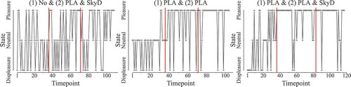
Summarized, the interventions appear to have increased the pleasure state membership and reduced the displeasure state membership, while leaving membership of the neutral state largely unaffected. It is noteworthy that participants receiving no intervention after the first month also slightly moved toward higher pleasure state membership and a lower displeasure state membership at that point in time. It appears that daily reflections on ones emotions also relieve anhedonia to a certain degree, which was already found in an intervention study using ESM in depressed patients (Kramer et al., 2014). Although these findings are merely exploratory and need to be validated in future research, we demonstrated that LMFA offers valuable insights to applied researchers.

Discussion

In this article, we introduced latent Markov factor analysis (LMFA) for modeling measurement model (MM) changes that are expected to be prevalent in time-intensive longitudinal data such as experience sampling data. In this way, LMFA safeguards conclusions about changes in the measured constructs. MM changes may pertain to (potentially interesting) substantive changes or may signal the onset of response styles (RSs). Between-state differences in intercepts and loadings might suggest an extreme RS, whereas differences in intercepts only rather suggest an agreeing RS (Cheung & Rensvold, 2000). When one suspects a RS in a specific state, RS detection and correction (e.g., adding an agreeing RS factor; Billiet & McClendon, 2000; Watson, 1992) can be applied to that specific part of the data, rather than to the entire data set. Moreover, the subject-specific transition probabilities of LMFA capture, for example, to what extent each subject is likely to end up and to stay in an extreme RS state. Even when RSs are hard to distinguish, the fact that LMFA pinpoints MM changes—and thus the reliable and comparable parts of the data—is valuable in itself.

In the future, it would be interesting to go beyond the purely exploratory approach applied in this article. On the one hand, hypothesis testing to determine which parameters significantly differ between the states might be preferred over visually comparing the state-specific MMs. To this end, LG already provides the researchers with Wald test statistics when the rotational freedom of the state-specific factors is resolved by a minimal number of restricted loadings (e.g., Geminiani, Ceulemans, & De Roover, 2018). On the other hand, including explanatory variables (i.e., time-constant or time-varying covariates such as personality traits or social contexts) in the model would allow to evaluate whether they significantly predict the state memberships and the transition probabilities.

Moreover, LMFA assumes normally distributed, continuous variables. However, categorical Likert-type scale ratings are frequently used in psychology. Although these data can often be treated as continuous in case of at least five response categories (Dolan, 1994; Olsson, 1979), the ratings are often skewed, thus violating the assumption of normality. Additionally, even continuous data, such as our application data, might be skewed. Therefore, the robustness of the method to such violations should be examined and, if necessary, possible extensions to deal with nonnormality should be considered.

In addition, longitudinal data are often collected in varying time intervals, for example, when testing the long-term influence of interventions on affect by collecting data in waves. In that case, the transition probabilities can no longer be considered time homogeneous, and continuous time modeling is necessary (Crayen, Eid, Lischetzke, & Vermunt, 2017). Therefore, in future research, we will develop a continuous-time extension of LMFA.

Moreover, a limitation of the method is the assumption that factor scores are centered around 0 and have a variance of 1. When factor scores evolve over time but the MM stays the same, changes in factor scores would currently be detected as intercept changes and thus possibly lead to different states according to model selection. In future work, we will investigate necessary LMFA extensions to explicitly model changes in factor means within the states, for example, depending on time or another covariate.

Next to that, we might consider an extension of LMFA using exploratory dynamic FA (EDFA; Browne, 2001; Zhang, 2006) within the states, which models the auto- and cross-lagged correlations of the factors at consecutive time-points but comes with important challenges. First, accurately estimating autocorrelations would require more measurement occasions per subject per state (Ram, Brose, & Molenaar, 2012), which may be undesirable. Second, in EDFA, factor rotation is more intricate since the auto- and cross-lagged relations between factors need to be rotated toward specified target matrices (Browne, 2001; Zhang, 2006), again necessitating the a priori hypotheses about (changes in) the MM we want to avoid. The LMM in LMFA already partly captures autocorrelations by the states, and uncaptured auto- and cross-lagged correlations will not necessarily introduce bias in the estimates of the state-specific MMs (Baltagi, 2011).

Finally, LMFA is a complex model with many assumptions. Therefore, misspecifications can occur, and tools to locate local misfit are essential. Local fit measures have been developed for related methods (e.g., bivariate residuals measures for multilevel data; Nagelkerke, Oberski, & Vermunt, 2016), but they need to be tailored and extensively evaluated for LMFA.

Additional information

Funding

The research leading to the results reported in this paper was sponsoredby the Netherlands Organization for Scientific Research (NWO) [ResearchTalent grant 406.17.517; Veni grant 451.16.004].

Notes

¹ Latent Markov factor analysis (LMFA) builds upon mixture simultaneous factor analysis (MSFA; De Roover et al., 2017), which captures differences in the factor model between groups. Whereas MSFA typically models the data of subjects nested within groups, LMFA specifically deals with observations nested within subjects, and it allows subjects to switch between different measurement models (MMs) over time.

² Note that the overview of existing methods focusses on FA-based methods and thus overlooks switching principal component analysis (SPCA; De Roover et al., 2014), which is a deterministic method similar to LMFA that can be used to take the first steps toward detecting MM changes over time, yet only for single-subject data. However, SPCA uses component instead of FA. Although components and factors are similar (Ogasawara, 2000; Velicer & Jackson, 1990; Velicer, Peacock, & Jackson, 1982), components do not correspond to latent variables (Borsboom, Mellenbergh, & van Heerden, 2003) and are thus less ideal for evaluating (changes in) MMs.

³ In total, participants rated their emotions three times a day with fixed 6-hr intervals. In the morning and midday, they rated their “momentary” emotions, and in the evening, they rated their emotions “since the last measure.” To have comparable and evenly spaced measures, we focused on the evening measures.

⁴ Missing data will be directly handled in the model estimation by considering only observed values.

⁵ A user-friendly graphical interface in LG including a tutorial will be developed in the future.

⁶ The “*” marks the subset of conditions that is included in the evaluation of model selection.

⁷ Note that we use exploratory factor analysis (EFA), and thus, the zero loadings are not fixed but freely estimated in LMFA.

⁸ Tucker’s (1951) congruence coefficient between column vectors x and y is defined as: .

⁹ We had no intention to evaluate the recovery of the initial state probabilities because more than a few subjects are required to validly estimate the distribution of initial starting states (Vermunt & Magidson, 2016). By sampling the initial state from a Bernoulli/multinomial distribution, some randomness in the initial states was obtained.

¹⁰ Note that rotation is not yet included in LG, which is why we take the estimated loadings and rotate them in the open-source program R (R Core Team, 2002).

¹¹ Note that, in case there is only one MM underlying the data, model selection would indicate that the one-state model fits best, which was confirmed by a small simulation study with the same design as the one of the model selection described in Section “Design and procedure.” The correct one-state model was correctly chosen for all 10 models (100%).

¹² Note that the NA items were mostly right skewed, warranting caution when drawing substantive conclusions because violations of the normality assumption have yet to be investigated (see Section “Discussion”). For the purpose of illustrating the aim of LMFA, this is not a problem.

¹³ The conditions marked by “*” are the ones that now have less levels than in simulation Study 1.

Appendix A

The model is estimated by means of the expectation maximization (EM; Dempster et al., 1977) algorithm that uses the so-called complete-data loglikelihood (), that is, assuming the state assignments of all time-points to be known and thus replacing the difficult maximization by a sequence of easier maximization problems. In the expectation step (E-step, see, for example, Bishop, 2006; Dias, Vermunt, & Ramos, 2008), we assume the parameters of interest (i.e., transition probabilities, initial probabilities, and state-specific MMs) to be given (i.e., by a set of initial values or estimates from the previous iteration , see De Roover et al., 2017; Vermunt & Magidson, 2016) and calculate the posterior probabilities (i.e., conditional on the data) to belong to each of the states and to make transitions between the states, by means of the forward–backward algorithm (Baum, Petrie, Soules, & Weiss, 1970). The obtained posterior probabilities are used as expected values of the state assignments to obtain the expected Next, in the maximization step (M-step), the parameters are updated such that is maximized. The E-step (Section “E-step”) and M-step (Section “M-step”) are iterated until convergence (Section “Convergence”).

E-step

The is given by

(A1)

Since the state memberships are in fact unknown, for each subject and time-point, the expected probability of being in a certain state and the expected probability of the occurrence of two consecutive states are inserted, in order to obtain ):

(A2)

The E-step for an LMC is achieved with the forward–backward (or Baum–Welch) algorithm (Baum et al., 1970). The algorithm finds the posterior probabilities by making use of the chain rule and the first-order Markov assumption: The joint probability of being in state k at time-point t and observing the sequence of observations can be expressed as

(A3)

The first-order Markov assumption implies that we can remove the dependency of the observations at time-point t on all previous observations and let them depend only on the state at time-point t. Thus, the equation reduces to

(A4)

The first factor refers to the forward probabilities and the second factor corresponds to the backward probabilities. On one hand, the forward probabilities, also indicated by , are the probabilities of observing and to end in state and are calculated by the forward algorithm. First, the initial state probabilities are used to calculate the forward probabilities for subject i of being in state k at time-point 1:

(A5)

Then, for the consecutive measurement occasions, we weight the forward probabilities of the previous time-point by the corresponding transition probabilities. Next, we sum over all possible ways (i.e., transitions) to come to a specific from any and multiply the values with the corresponding response probabilities:

(A6)

On the other hand, the backward probabilities, also indicated by , are the probabilities to be in state and to generate the remaining sequence . Instead of starting at time-point 1, the so called backward algorithm starts at time-point T and backtracks to time-point t + 1. The probability for the backward algorithm to be in the final state and, thus, to produce no outcome (anymore is assumed to be 1:

(A7)

Henceforth, the backward probabilities can be determined in a similar way as the forward probabilities. However, as we go backwards here, we now need to consider the response probabilities of all K states at time-point , multiplying them with the backward probabilities and the respective transition probabilities, prior to summing over K:

(A8)

Next, (Equation (A4)) is calculated by multiplying the forward and the backward probabilities:

(A9)

Subsequently, we can calculate the conditional probability of being in state given the sequence of observations, as we know that

(A10)

By inserting this into Equation (A9), we obtain

(A11)

It follows that the conditional state probability is equal to

(A12)

The denominator can be calculated by marginalizing Equation (A9) to by summing over the latent states for an arbitrarily chosen t:

(A13)

which is in its simplest form for t = T, where . Thus, the equation reduces to

(A14)

Finally, we can calculate the joint probability of two successive states by applying Bayes’ theorem:

(A15)

M-step

In the M-step, we maximize with respect to . To maximize, we set the derivatives with respect to the parameters to zero, making use of Lagrange multipliers whenever a constraint, such as , needs to be satisfied. The resulting updates are as follows:

(A16)

(A17)

(A18)

The factor models for the state-specific covariance matrices are estimated by another maximization algorithm within each M-step. Specifically, each observation is weighted by the corresponding -value, resulting in K weighted data sets . Fisher scoring (Lee & Jennrich, 1979; Vermunt & Magidson, 2016) is used to perform factor analysis on these weighted data.

Convergence

The convergence can be evaluated either with respect to the or with respect to the parameter estimates. LG applies the latter approach and assesses convergence by computing the following quantity:

(A19)

which is the sum of the absolute values of the relative parameter changes where refers to the parameters. In this article, the stopping criterion is . The estimation also stops if the change in the becomes smaller than prior to reaching the stopping criterion above.

Appendix B

//LG5.1//

version = 5.1

infile 'Sim1.csv' quote = single

model

options

algorithm

tolerance = 1e-008 emtolerance = 1e-008 emiterations = 3000 nriterations = 0;

startvalues

seed = 0 sets = 25 tolerance = 1e-005 iterations = 100 PCA;

bayes latent = 0;

montecarlo

seed = 0 replicates = 500 tolerance = 1e-008;

quadrature nodes = 10;

missing includeall;

output

profile parameters standarderrors estimatedvalues classification probmeans iterationdetails

WriteParameters = 'results_parameters.csv'

write = 'results.csv'

writeloadings = 'results_loadings.txt';

outfile

'classification.csv' classification;

variables

caseid id;

dependent

V1 continuous, V2 continuous, V3 continuous, V4 continuous, V5 continuous, V6 continuous, V7 continuous, V8 continuous, V9 continuous, V10 continuous, V11 continuous, V12 continuous, V13 continuous, V14 continuous, V15 continuous, V16 continuous, V17 continuous, V18 continuous, V19 continuous, V20 continuous;

latent

State nominal dynamic coding = first 2,

F1 continuous dynamic,

F2 continuous dynamic;

independent id nominal;

equations

//factor variances

(1) F1| State;

(1) F2| State;

//Markov model

State[=0] <- 1;

State <- (~tra) 1 | State[−1] id;

//regression models for items

V1-V20 <- 1 | State + F1 | State + F2 | State;

//unique variances

V1-V20 | State;

end model

Appendix C

Problem of the Additional Simulation Study

To test whether lag-one autocorrelations of factors not captured by the within-state EFA analyses harm the performance of LMFA, we manipulated factors (a)–(g) as in the main simulation study, leaving out the levels with an already inferior performance, and added an eighth factor (h) specifying the autocorrelation.

Design and Procedure

We crossed eight factors in a complete factorial design¹³:

a. number of factors per state F^k at two levels: 2, 4;

b. number of states at three levels: 2, 4*;

c. between state difference at two levels:

  medium loading difference and low intercept difference,

  medium loading difference and medium intercept difference*;

d. unique variance : fixed at 0.2, 0.4;

e. frequency of transitions between the states at two levels: frequent, infrequent*;

f. number of subjects at three levels: 2, 10*;

g. number of observations per subject per state at three levels: 50, 100, 200;

h. autocorrelation at three levels: 0, 0.3, 0.7*

The data were generated by means of the orthogonal dynamic factor model which implies that, at time-point t, the factors are uncorrelated with one another but a factor’s scores at time-point t are dependent on its scores at time-point t − 1. Specifically, they are autocorrelated by the coefficient as follows:

(C1)

where is a subject-specific F^k × 1 vector of noise at time-point t which is assumed to be multivariate normally distributed with zero mean and the identity matrix as covariance matrix (~. Thus, to generate the subject-specific data sets , first, the and vectors were sampled for each observation. Subsequently, we created the autocorrelated factor score vectors by applying a recursive filter (Hamilton, 1994). This filter sets the first noise element as the first factor score and computes the remaining factor scores as in Equation (C1). The resulting factor scores were multiplied by to retain an expected variance of 1 (De Roover, Timmerman, Van Diest, Onghena, & Ceulemans, 2014). Finally, the data-matrices were again merged into one data set . Note that, for the strength of the autocorrelation (h), we used the values suggested by Cabrieto, Tuerlinckx, Kuppens, Grassmann, and Ceulemans (2017). To check how the manipulation played out, we calculated the average autocorrelation across the data sets for each of the three conditions: they amounted to 0.05, 0.29, and 0.68.

For each cell of the factorial design, 20 data sets were generated as described above. In total 2 (number of states) × 2 (number of factors) × 2 (between-state difference) × 2 (transition frequency between states) × 2 (number of subjects) × 3 (number of observations per subject and state) × 2 (unique variance) × 3 (autocorrelation) × 20 (replicates) = 5760 simulated data sets were generated. As in Simulation Study 1, the data were generated in R and analyzed in LG with the same settings and the correct number of states and factors per state.

Results

In general, the recovery was largely unaffected by the autocorrelation conditions (h). Specifically, the recovery of the transition matrices and unique variances was not affected − MAD_trans = 0.05 and MAD_uniq = 0.03 for —whereas the recovery of the states, loadings, and intercepts was only slightly affected—for and for ; for and for ; forfor and for . Note that the mild decrease in intercept recovery with an increased autocorrelation is merely a consequence of the higher variance of the estimated intercepts, since they capture part of the autocorrelation and thus vary more around the population values.

References

- Adolf, J., Schuurman, N. K., Borkenau, P., Borsboom, D., & Dolan, C. V. (2014). Measurement invariance within and between individuals: A distinct problem in testing the equivalence of intra- and inter-individual model structures. Frontiers in Psychology, 5, 883. doi:10.3389/fpsyg.2014.00883
- American Psychiatric Association. (2013). Diagnostic and statistical manual of mental disorders (5th ed.). Arlington, VA: American Psychiatric Publishing.
- Asparouhov, T., Hamaker, E. L., & Muthen, B. (2017). Dynamic structural equation models. Technical Report.
- Baltagi, B. H. (2011). Econometrics (5th ed.). Berlin, Germany: Springer.
- Bartolucci, F. (2006). Likelihood inference for a class of latent Markov models under linear hypotheses on the transition probabilities. Journal of the Royal Statistical Society, Series B, 68, 155–178. doi:10.1111/j.1467-9868.2006.00538.x
- Bartolucci, F., Farcomeni, A., & Pennoni, F. (2014). Comments on: Latent Markov models: A review of a general framework for the analysis of longitudinal data with covariates. Test, 23, 473–477. doi:10.1007/s11749-014-0387-1
- Bartolucci, F., Farcomeni, A., & Pennoni, F. (2015). Latent Markov models for longitudinal data. Hoboken, NJ: CRC Press.
- Baum, L. E., Petrie, T., Soules, G., & Weiss, N. (1970). A maximization technique occurring in the statistical analysis of probabilistic functions of Markov chains. Annals of Mathematical Statistics, 41, 164–171. doi:10.1214/aoms/1177697196
- Berridge, K. C., Robinson, T. E., & Aldridge, J. W. (2009). Dissecting components of reward: ‘liking’, ‘wanting’, and learning. Current Opinion in Pharmacology, 9, 65–73. doi:10.1016/j.coph.2008.12.014
- Billiet, J. B., & McClendon, M. J. (2000). Modeling acquiescence in measurement models for two balanced sets of items. Structural Equation Modeling: A Multidisciplinary Journal, 7(4), 608–628. doi:10.1207/s15328007sem0704_5
- Bishop, C. M. (2006). Pattern recognition and machine learning (5th ed.). New York, NY: Springer.
- Borsboom, D., Mellenbergh, G. J., & van Heerden, J. (2003). The theoretical status of latent variables. Psychological Review, 110, 203–219. doi:10.1037/0033-295X.110.2.203
- Briggs, N. E., & MacCallum, R. C. (2003). Recovery of weak common factors by maximum likelihood and ordinary least squares estimation. Multivariate Behavioral Research, 38(1), 25–56. doi:10.1207/S15327906MBR3801_2
- Browne, M. W. (2001). An overview of analytic rotation in exploratory factor analysis. Multivariate Behavioral Research, 36, 111–150. doi:10.1207/S15327906MBR3601_05
- Cabrieto, J., Tuerlinckx, F., Kuppens, P., Grassmann, M., & Ceulemans, E. (2017). Detecting correlation changes in multivariate time series: a comparison of four non-parametric change point detection methods. Behavior Research Methods, 49, 988–1005. doi: 10.3758/s13428-016-0754-9
- Carvalho, C. M., & Lopes, H. F. (2007). Simulation-based sequential analysis of Markov switching stochastic volatility models. Computational Statistics & Data Analysis, 51, 4526–4542. doi:10.1016/j.csda.2006.07.019
- Cheung, G. W., & Rensvold, R. B. (2000). Assessing extreme and acquiescence response sets in cross-cultural research using structural equations modeling. Journal of Cross-Cultural Psychology, 31, 187–212. doi:10.1177/0022022100031002003
- Clarkson, D. B., & Jennrich, R. I. (1988). Quartic rotation criteria and algorithms. Psychometrica, 53, 251–259. doi:10.1007/BF02294136
- Collins, L. M., & Lanza, S. T. (2010). Latent class and latent transition analysis: With applications in the social, behavioral, and health sciences. New York, NY: Wiley.
- Crayen, C., Eid, M., Lischetzke, T., & Vermunt, J. K. (2017). A continuous-time mixture latent-state-trait Markov model for experience sampling data. European Journal of Psychological Assessment, 33, 296–311. doi:10.1027/1015-5759/a000418
- De Roover, K., Timmerman, M. E., Van Diest, I., Onghena, P., & Ceulemans, E. (2014). Switching principal component analysis for modeling means and covariance changes over time. Psychological Methods, 19, 113–132. doi:10.1037/a0034525
- De Roover, K., Vermunt, J. K., Timmerman, M. E., & Ceulemans, E. (2017). Mixture simultaneous factor analysis for capturing differences in latent variables between higher level units of multilevel data. Structural Equation Modeling: A Multidisciplinary Journal, 24, 1–18. doi:10.1080/10705511.2017.1278604
- de Winter, J. C., Dodou, D., & Wieringa, P. A. (2009). Exploratory factor analysis with small sample sizes. Multivariate Behavioral Research, 44, 147–181. doi:10.1080/00273170902794206
- Dempster, A. P., Laird, N. M., & Rubin, D. B. (1977). Maximum likelihood from incomplete data via the EM algorithm. Journal of the Royal Statistical Society. Series B (Methodological), 39, 1–38.
- Dias, J. G., Vermunt, J. K., & Ramos, S. (2008). Heterogeneous hidden Markov models: COMPSTAT 2008 Proceedings, Porto, Portugal: Physica.
- Dolan, C. V. (1994). Factor analysis of variables with 2, 3, 5 and 7 response categories: A comparison of categorical variable estimators using simulated data. British Journal of Mathematical and Statistical Psychology, 47, 309–326. doi:10.1111/bmsp.1994.47.issue-2
- Feldman, L. A. (1995). Valence focus and arousal focus: Individual differences in the structure of affective experience. Journal of Personality and Social Psychology, 69, 153–166. doi:10.1037/0022-3514.69.1.153
- Geminiani, E., Ceulemans, E., & De Roover, K. (2018). Wald tests for factor loading differences among many groups: Power and type I error. Manuscript submitted for publication.
- Grühn, D., Lumley, M. A., Diehl, M., & Labouvie-Vief, G. (2013). Time-based indicators of emotional complexity: Interrelations and correlates. Emotion (Washington, D.C.), 13, 226–237. doi:10.1037/a0030363
- Hagenaars, J. A., & McCutcheon, A. L. (Eds.). (2002). Applied latent class analysis. New York, NY: Cambridge University Press.
- Hamilton, J. D. (1994). Time series analysis. Princeton, NJ: Princeton University Press.
- Heininga, V. E., Van Roekel, E., Ahles, J. J., Oldehinkel, A. J., & Mezulis, A. H. (2017). Positive affective functioning in anhedonic individuals’ daily life: Anything but flat and blunted. Journal of Affective Disorders, 218, 437–445. doi:10.1016/j.jad.2017.04.029
- Hubert, L., & Arabie, P. (1985). Comparing partitions. Journal of Classification, 2, 193–218. doi:10.1007/BF01908075
- Jolliffe, I. T. (1986). Principal component analysis. NewYork, NY: Springer.
- Kaiser, H. F. (1958). The varimax criterion for analytic rotation in factor analysis. Psychometrika, 23, 187–200. doi:10.1007/BF02289233
- Kang, X., & Thakor, N. V. (2012). Factor analyzed hidden Markov models for estimating prosthetic limb motions using premotor cortical ensembles. Paper presented at the IEEE RAS/EMBS International Conference on Biomedical Robotics and Biomechatronics, Roma, Italy.
- Kiers, H. A. (1997). Techniques for rotating two or more loading matrices to optimal agreement and simple structure: A comparison and some technical details. Psychometrika, 62, 545–568. doi:10.1007/BF02294642
- Kramer, I., Simons, C. J. P., Hartmann, J. A., Menne-Lothmann, C., Viechtbauer, W., Peeters, F., … Wichers, M. (2014). A therapeutic application of the experience sampling method in the treatment of depression: A randomized controlled trial. World Psychiatry : Official Journal of the World Psychiatric Association (WPA), 13, 68–77. doi:10.1002/wps.20090
- Larson, R., & Csikszentmihalyi, M. (2014). The experience sampling method. In M. Csikszentmihalyi (Ed.), Flow and the foundations of positive psychology (pp. 21–34). Dordrecht, The Netherlands: Springer.
- Lawley, D. N., & Maxwell, A. E. (1962). Factor analysis as a statistical method. London, UK: Butterworth.
- Lazarsfeld, P. F., & Henry, N. W. (1968). Latent structure analysis. New York, NY: Houghton Mifflin.
- Lee, S. Y., & Jennrich, R. I. (1979). A study of algorithms for covariance structure analysis with specific comparisons using factor analysis. Psychometrika, 44, 99–113. doi:10.1007/BF02293789
- Little, T. D., Preacher, K. J., Selig, J. P., & Card, N. A. (2007). New developments in latent variable panel analyses of longitudinal data. International Journal of Behavioral Development, 31, 357–365. doi:10.1177/0165025407077757
- Lopes, H. F., & West, M. (2004). Bayesian model assessment in factor analysis. Statistica Sinica, 14, 41–67.
- MacCallum, R. C., Widaman, K. F., Preacher, K. J., & Hong, S. (2001). Sample size in factor analysis: The role of model error. Multivariate Behavioral Research, 36, 611–637. doi:10.1207/S15327906MBR3604_06
- MacCallum, R. C., Widaman, K. F., Zhang, S., & Hong, S. (1999). Sample size in factor analysis. Psychological Methods, 4, 84–99. doi:10.1037/1082-989X.4.1.84
- McDonald, R. P., & Krane, W. R. (1979). A Monte Carlo study of local identifiability and degrees of freedom in the asymptotic likelihood ratio test. British Journal of Mathematical and Statistical Psychology, 32, 121–132. doi:10.1111/j.2044-8317.1979.tb00757.x
- Meredith, W. (1993). Measurement invariance, factor analysis and factorial invariance. Psychometrika, 58, 525–543. doi:10.1007/BF02294825
- Meredith, W., & Teresi, J. A. (2006). An essay on measurement and factorial invariance. Medical Care, 44, 69–77. doi:10.1097/01.mlr.0000245438.73837.89
- Moors, G. (2003). Diagnosing response style behavior by means of a latent-class factor approach. Socio-demographic correlates of gender role attitudes and perceptions of ethnic discrimination reexamined. Quality and Quantity, 37, 277–302. doi:10.1023/A:1024472110002
- Morren, M., Gelissen, J. P., & Vermunt, J. K. (2011). Dealing with extreme response style in cross‐cultural research: A restricted latent class factor analysis approach. Sociological Methodology, 41, 13–47. doi:10.1111/j.1467-9531.2011.01238.x
- Myung, I. J. (2003). Tutorial on maximum likelihood estimation. Journal of Mathematical Psychology, 47, 90–100. doi:10.1016/s0022-2496(02)00028-7
- Nagelkerke, E., Oberski, D. L., & Vermunt, J. K. (2016). Power and type I error of local fit statistics in multilevel latent class analysis. Structural Equation Modeling: A Multidisciplinary Journal, 24, 216–229. doi:10.1080/10705511.2016.1250639
- Ogasawara, H. (2000). Some relationships between factors and components. Psychometrika, 65, 167–185. doi:10.1007/BF02294372
- Olsson, U. (1979). On the robustness of factor analysis against crude classification of the observations. Multivariate Behavioral Research, 14, 481–500. doi:10.1207/s15327906mbr1404_7
- Oort, F. J., Visser, M. R., & Sprangers, M. A. (2005). An application of structural equation modeling to detect response shifts and true change in quality of life data from cancer patients undergoing invasive surgery. Quality of Life Research, 14, 599–609. doi:10.1007/s11136-004-0831-x
- Paulhus, D. L. (1991). Measures of personality and social psychological attitudes. In J. P. Robinson & R. P. Shaver (Eds.), Measures of social psychological attitudes series (Vol. 1, pp. 17–59). San Diego, CA: Academic Press.
- Preacher, K. J., & MacCallum, R. C. (2002). Exploratory factor analysis in behavior genetics research: Factor recovery with small sample sizes. Behavior Genetics, 32, 153–161. doi:10.1023/A:1015210025234
- R Core Team. (2002). A language and environment for statistical computing. Vienna, Austria: R Foundation for Statistical Computing. Retrieved from https://www.R-project.org/
- Ram, N., Brose, A., & Molenaar, P. C. M. (2012). Dynamic factor analysis: Modeling person-specific process. In T. D. Little (Ed.), The Oxford handbook of quantitative methods (Vol. 2, pp. 441–457). New York, NY: Oxford University Press.
- Rindskopf, D. (1984). Structural equation models: Empirical identification, Heywood cases, and related problems. Sociological Methods & Research, 13, 109–119. doi:10.1177/0049124184013001004
- Rosti, A. I., & Gales, M. J. (2002). Factor analysed hidden Markov models: ICASSP 2002 proceedings (Vol. 1, pp. 949–952). Florida: IEEE.
- Schaie, K. W., Maitland, S. B., Willis, S. L., & Intrieri, R. C. (1998). Longitudinal invariance of adult psychometric ability factor structures across 7 years. Psychology and Aging, 13, 8–20. doi:10.1080/13825580490511134
- Scollon, C., Kim-Prieto, C., & Diener, E. (2003). Experience sampling: Promises and pitfalls, strengths and weaknesses. Journal of Happiness Studies, 4, 5–34. doi:10.1023/A:1023605205115
- Song, X., Xia, Y., & Zhu, H. (2017). Hidden Markov latent variable models with multivariate longitudinal data. Biometrics, 73, 313–323. doi:10.1111/biom.12536
- Steinley, D. (2004). Properties of the hubert-arabie adjusted rand index. Psychological Methods, 9, 386–396. doi:10.1037/1082-989X.9.3.386
- Steinley, D., & Brusco, M. J. (2011). Evaluating mixture modeling for clustering: Recommendations and cautions. Psychological Methods, 16, 63–79. doi:10.1037/a0022673
- Stevens, J. (1992). Applied multivariate statistics for the social sciences. Hillsdale, NJ: Lawrence Erlbaum Associates.
- Treadway, M. T., & Zald, D. H. (2011). Reconsidering anhedonia in depression: Lessons from translational neuroscience. Neuroscience and Biobehavioral Reviews, 35, 537–555. doi:10.1016/j.neubiorev.2010.06.006
- Tucker, L. R. (1951). A method for synthesis of factor analysis studies. Personnel Research Section Report No. 984. Washington, DC: Department of the Army.
- Van Driel, O. P. (1978). On various causes of improper solutions in maximum likelihood factor analysis. Psychometrika, 43, 225–243. doi:10.1007/BF02293865
- van Roekel, E., Bennik, E. C., Bastiaansen, J. A., Verhagen, M., Ormel, J., Engels, R. C., & Oldehinkel, A. J. (2015). Depressive symptoms and the experience of pleasure in daily life: An exploration of associations in early and late adolescence. Journal of Abnormal Child Psychology, 44, 999–1009. doi:10.1007/s10802-015-0090-z
- Van Roekel, E., Vrijen, C., Heininga, V. E., Masselink, M., Bos, E. H., & Oldehinkel, A. J. (2017). An exploratory randomized controlled trial of personalized lifestyle advice and tandem skydives as a means to reduce anhedonia. Behavior Therapy, 48, 76–96. doi:10.1016/j.beth.2016.09.009
- Velicer, W. F., & Fava, J. L. (1998). Affects of variable and subject sampling on factor pattern recovery. Psychological Methods, 3, 231–251. doi:10.1037/1082-989X.3.2.231
- Velicer, W. F., & Jackson, D. N. (1990). Component analysis versus common factor analysis: Some issues in selecting an appropriate procedure. Multivariate Behavioral Research, 25, 1–28. doi:10.1207/s15327906mbr2501_1
- Velicer, W. F., Peacock, A. C., & Jackson, D. N. (1982). A comparison of component and factor patterns: A Monte Carlo approach. Multivariate Behavioral Research, 17, 371–388. doi:10.1207/s15327906mbr1703_5
- Vermunt, J. K., Langeheine, R., & Böckenholt, U. (1999). Discrete-time discrete-state latent markov models with time constant and time-varying covariates. Journal of Educational and Behavioral Statistics, 24, 179–207. doi:10.2307/1165200
- Vermunt, J. K., & Magidson, J. (2016). Technical guide for latent GOLD 5.1: Basic, advanced, and syntax. Belmont, MA: Statistical Innovations.
- Watson, D. (1992). Correcting for acquiescent response bias in the absence of a balanced scale. Sociological Methods & Research, 21, 52–88. doi:10.1177/0049124192021001003
- Xia, Y.-M., Tang, N.-S., & Gou, J.-W. (2016). Generalized linear latent models for multivariate longitudinal measurements mixed with hidden Markov models. Journal of Multivariate Analysis, 152, 259–275. doi:10.1016/j.jmva.2016.09.001
- Ximenez, C. (2009). Recovery of weak factor loadings in confirmatory factor analysis under conditions of model misspecification. Behavior Research Methods, 41, 1038–1052. doi:10.3758/BRM.41.4.1038
- Ximénez, C. (2006). A Monte Carlo study of recovery of weak factor loadings in confirmatory factor analysis. Structural Equation Modeling, 13, 587–614. doi:10.1207/s15328007sem1304_5
- Zhang, G. (2006). Bootstrap Procedures for Dynamic Factor Analysis. Unpublished doctoral dissertation. The Ohio State University, Columbus, OH.