Sample Size Recommendations for Continuous-Time Models: Compensating Shorter Time Series with Larger Numbers of Persons and Vice Versa

ABSTRACT

Autoregressive modeling has traditionally been concerned with time-series data from one unit (N = 1). For short time series (T < 50), estimation performance problems are well studied and documented. Fortunately, in psychological and social science research, besides T, another source of information is often available for model estimation, that is, the persons (N > 1). In this work, we illustrate the N/T compensation effect: With an increasing number of persons N at constant T, the model estimation performance increases, and vice versa, with an increasing number of time points T at constant N, the performance increases as well. Based on these observations, we develop sample size recommendations in the form of easily accessible N/T heatmaps for two popular autoregressive continuous-time models.

KEYWORDS:

• Continuous-time modeling
• intensive longitudinal data
• sample size
• time series

Modeling intensive longitudinal data is clearly a challenge that more and more researchers face because intensive longitudinal methods, such as the experience sampling method (ESM), ecological momentary assessment (EMA), and ambulatory assessment (AA), become more and more popular. These methods usually produce unequally spaced data with varying time interval lengths between successive measurement occasions. One natural choice for this kind of data is continuous-time modeling because an underlying continuous process is assumed of which the measurements at discrete points in time are snapshots (Hecht et al., 2019).

Continuous-time models belong to the broad class of autoregressive models which are very popular in economic research and econometrics to analyze time-series data such as gross national products, sales prices of houses, number of passengers, market shares of toothpastes, and chemical process concentrations (Bisgaard & Kulahci, 2011, Chapter 1.2), to name just a few examples. Usually, a large number of observations (i.e., time points $T$) are available in these research areas. In psychological research, however, the number of time points is often rather small because repeatedly obtaining data from a person is more cost-intensive than, for example, gathering the market price of a stock. Unfortunately, short time series are a known issue for model estimation as numerous studies have shown (e.g., Arnau & Bono, 2001; DeCarlo & Tryon, 1993; Huitema & McKean, 1991, 1994; Krone et al., 2017; Solanas et al., 2010). The general finding is that estimation performance increases with an increasing number of time points. For instance, Krone et al. (2017) studied the estimation performance of the autoregressive parameter for a range of $T$ between 10 and 100 and found that “… the bias becomes smaller as $T$ increases …” (p. 10), the bias of the standard error of the autoregressive parameter decreases when $T$ becomes larger (p. 12), “… the empirical rejection rate approaches the nominal $\alpha$ as the length of the time series increases …” (p. 13), and that the power of the estimated autoregressive parameter shows a positive relation to the size of $T$ (p. 14). Recommendations on the minimum necessary number of time points for time-series analysis vary, however, there is considerable consensus that this minimum requirement is in the middle two-digit range, for instance, “… 40 observations is often mentioned as the minimum number of observations for a time-series analysis” (Poole et al., 2002, p. 56), “… many models require at least 50 observations for accurate estimation (McCleary et al., 1980, p. 20).” (Jebb et al., 2015, p. 3), “Most time-series experts suggest that the use of time-series analysis requires at least 50 observations in the time series.” (Warner, 1998, pp. 2–3).

Whereas time-series analysis in economic research and econometrics is often concerned with a single unit, in the social sciences (e.g., psychology), we are commonly dealing with more than one, usually many, units (i.e., persons). Thus, besides time points, we have persons as another source of information for model estimation. In analogy to the well-proven positive effects of a larger number of time points $T$ on estimation performance, it is reasonable to assume a similar effect for an increasing number of persons $N$. Assuming that persons are—at least to some degree—alike, adding persons can add information for the estimation of the parameters of autoregressive models. Thus, it would be possible to compensate for smaller $T$ with larger $N$ and vice versa. Such effects are described by Schultzberg and Muthén (2018) and support for adding more information via increasing $N$ and $T$ is also suggested by Oud et al. (2018, p. 4) and Hecht et al. (2019, p. 528).

The mechanism behind such compensation effects can be described from different angles.¹ The assumption of a common probability distribution of individual parameters provides information, for instance, the range in which the individual parameters are concentrated. Because the individuals contribute information to the common distribution and this distribution, in turn, informs the individual parameter estimation, one person is to some extent informative for another. From a Bayesian perspective, the common distribution can be seen as a form of prior distribution. Viewed from a regularization perspective, the prior can regularize the model and thus attenuate overfitting issues (Bulteel et al., 2018).

In summary, the information that persons add for model estimation can be “connected” and therefore utilized for better parameter estimation by introducing assumptions about the common distribution of individual parameters. This mechanism fuels the $N$/$T$ compensation effect because increasing $N$ and/or $T$ leads to more such information.

Purpose and scope

In the present work, we investigate the performance of a univariate continuous-time autoregressive model as a function of $N$ and $T$. The first objective is to demonstrate the suggested $N$/$T$ compensation effect on estimation performance. To this end, we present results from simulations with varying $T$ for $N$ = 1 and $N$ > 1. The assumption for this demonstration was that persons are identical, that is, there is no between-person variation in any model parameters. The second objective is to derive sample size recommendations. As persons usually differ in their mean level, we present results for a continuous-time model including between-person variance in the process means. This is the continuous-time univariate version of the popular cross-lagged panel model (e.g., Kearney, 2017; Selig & Little, 2012) with random intercepts (Hamaker et al., 2015) and one of the building blocks for more complex models for unequally spaced ESM/EMA/AA data analysis. Our results can be used as guidance for choosing an $N$/$T$ combination with sufficient performance.

The article is organized into the following sections. First, we briefly present the univariate continuous-time model. Second, we report results from a simulation study in which we varied the number of time points and the number of persons and assessed convergence rate, relative bias, and coverage rate as estimation performance criteria. Finally, we conclude with a discussion of our work. Annotated R code for estimating the employed continuous-time models with the R package ctsem (Driver et al., 2017) is provided in the supplementary material.

The univariate continuous-time model

We adapt the continuous-time model formulation from Hecht and Zitzmann (2020) which is based on the work of Oud and Delsing (2010) and Hecht et al. (2019). Unequal-interval longitudinal designs involve responses of $j=1,\dots ,N$ persons at several points in time, $t_p$, with $p=1,\dots ,T$ being a running index denoting the discrete time point and $T$ being the number of time points. Time interval lengths ${\mathrm{\Delta }}_{p-1}$ between time points are given by ${\mathrm{\Delta }}_{p-1}=t_p-t_{p-1}$ for all $p\ge 2$, and $y_{jp}$ is the value of person $j$ on the variable $y$ at time point $p$. The continuous-time model is given by:

(1) $\text{for }p\ge 2,y_{jp}=a_{{\Delta }_{p-1}}^{*}{y}_{j(p-1)}+\left(1-a_{{\Delta }_{p-1}}^{*}\right){\mu }_{j{\infty }_{+}^{*}}{\omega }_{j(p-1)},$(1)

(2) $a_{{\mathrm{\Delta }}_{p-1}}^{\ast }=exp(a{\mathrm{\Delta }}_{p-1}),$(2)

(3) ${\mu }_{j\mathrm{\infty }}^{\ast }\sim \mathcal{N}\left({\mu }_{\mathrm{\infty }}^{\ast },{\sigma }_{\mathrm{\infty }}^{2^{\ast }}\right),$(3)

(4) $\hspace{0.17em}{\omega }_{j(p-1)}\sim \mathcal{N}\left(0,q_{{\mathrm{\Delta }}_{p-1}}^{\ast }\right),$(4)

(5) $q_{{\mathrm{\Delta }}_{p-1}}^{\ast }=-\left[exp(2a{\mathrm{\Delta }}_{p-1})-1\right]q_{\mathrm{\infty }}^{\ast },$(5)

(6) $\mathrm{a}\mathrm{n}\mathrm{d}\mathrm{f}\mathrm{o}\mathrm{r}p=1,y_{j1}\sim \mathcal{N}\left({\mu }_{j\mathrm{\infty }}^{\ast }+{\mu }_{\mathrm{d}\mathrm{e}\mathrm{v}},{\sigma }_{\mathrm{f}\mathrm{w}}^2\right),$(6)

where $a_{{\mathrm{\Delta }}_{p-1}}^{\ast }$ are the discrete-time autoregressive effects that depend on the continuous-time auto-effect $a$ and the time interval length (Equation 2(2) $a_{{\mathrm{\Delta }}_{p-1}}^{\ast }=exp(a{\mathrm{\Delta }}_{p-1}),$(2) )²; ${\mu }_{j\mathrm{\infty }}^{\ast }$ are the long-range person-specific process means which are normally distributed with mean ${\mu }_{\mathrm{\infty }}^{{ }^{\ast }}$ and variance ${\sigma }_{\mathrm{\infty }}^{2^{\ast }}$ (Equation 3(3) ${\mu }_{j\mathrm{\infty }}^{\ast }\sim \mathcal{N}\left({\mu }_{\mathrm{\infty }}^{\ast },{\sigma }_{\mathrm{\infty }}^{2^{\ast }}\right),$(3) ); ${\omega }_{j(p-1)}$ are the person- and time point-specific process error terms which are normally distributed with zero mean and variance $q_{{\mathrm{\Delta }}_{p-1}}^{\ast }$ (Equation 4(4) $\hspace{0.17em}{\omega }_{j(p-1)}\sim \mathcal{N}\left(0,q_{{\mathrm{\Delta }}_{p-1}}^{\ast }\right),$(4) ), with $q_{{\mathrm{\Delta }}_{p-1}}^{\ast }$ depending on the within-person long-range process variance $q_{\mathrm{\infty }}^{\ast }$, the auto-effect $a$, and on the time interval length (Equation 5(5) $q_{{\mathrm{\Delta }}_{p-1}}^{\ast }=-\left[exp(2a{\mathrm{\Delta }}_{p-1})-1\right]q_{\mathrm{\infty }}^{\ast },$(5) ). The values at the first time point, $y_{j1}$, are normally distributed with variance ${\sigma }_{\mathrm{f}\mathrm{w}}^2$ and mean ${\mu }_{j\mathrm{\infty }}^{\ast }+{\mu }_{\mathrm{d}\mathrm{e}\mathrm{v}}$, where ${\mu }_{\mathrm{d}\mathrm{e}\mathrm{v}}$ is the deviation of the mean at the first time point from the overall process mean ${\mu }_{\mathrm{\infty }}^{\ast }$. Figure 1 illustrates this continuous-time model for three time points. For more explanations, examples, and illustrations of this (and other) continuous-time models see Hecht and Zitzmann (2020), Hecht et al. (2019), Hecht and Voelkle (2019), Driver et al. (2017), Driver and Voelkle (2018), and Voelkle et al. (2012).

Figure 1. The univariate continuous-time model with three time points. Model parameters that are estimated are set in light text color on a dark background

Simulation study

Simulation design

In our simulation study, we estimated continuous-time models for three scenarios: (1) one person ($N$ = 1), (2) multiple identical persons (no between-person variation in process means; that is, intra-class correlation ICC = 0), and (3) multiple persons who differ in individual process means (ICC = 0.50). For all scenarios, we varied the number of time points: $T$ = 3, 4, 5, 7, 10, 15, 20, 30, 50, 75, 100, 150, or 250. For scenarios 2 and 3, we varied the number of persons as well: $N$ = 5, 25, 50, 100, 250, 500, 1,000, or 2,500, and fully crossed $N$ and $T$, which resulted in 104 $N$/$T$ combinations.

Data generation

The data-generating model was the univariate continuous-time model described in Equations 1(1) $\text{for }p\ge 2,y_{jp}=a_{{\Delta }_{p-1}}^{*}{y}_{j(p-1)}+\left(1-a_{{\Delta }_{p-1}}^{*}\right){\mu }_{j{\infty }_{+}^{*}}{\omega }_{j(p-1)},$(1) to 6(6) $\mathrm{a}\mathrm{n}\mathrm{d}\mathrm{f}\mathrm{o}\mathrm{r}p=1,y_{j1}\sim \mathcal{N}\left({\mu }_{j\mathrm{\infty }}^{\ast }+{\mu }_{\mathrm{d}\mathrm{e}\mathrm{v}},{\sigma }_{\mathrm{f}\mathrm{w}}^2\right),$(6) and depicted in Figure 1. For all scenarios, the true parameter values were $a=-0.40$, ${\mu }_{\mathrm{\infty }}^{\ast }=1$, $q_{\mathrm{\infty }}^{\ast }=0.50$, ${\mu }_{\mathrm{d}\mathrm{e}\mathrm{v}}=1$, and ${\sigma }_{\mathrm{f}\mathrm{w}}^2=0.50$. In scenario 1 (one person) and 2 (multiple identical persons), there is no between-person variance in process means, therefore: ${\mu }_{j\mathrm{\infty }}^{\ast }={\mu }_{\mathrm{\infty }}^{\ast }$. In scenario 3, the true between-person variance in process means was ${\sigma }_{\mathrm{\infty }}^{2^{\ast }}=0.50$, implying an intra-class correlation of $\mathrm{I}\mathrm{C}\mathrm{C}={\sigma }_{\mathrm{\infty }}^{2^{\ast }}/({\sigma }_{\mathrm{\infty }}^{2^{\ast }}+q_{\mathrm{\infty }}^{\ast })=0.50$. The full data-generating model is:

$\mathrm{f}\mathrm{o}\mathrm{r}\mathrm{s}\mathrm{c}\mathrm{e}\mathrm{n}\mathrm{a}\mathrm{r}\mathrm{i}\mathrm{o}\mathrm{s}1\mathrm{a}\mathrm{n}\mathrm{d}2,{\mu }_{j\mathrm{\infty }}^{\ast }=1,$

$\mathrm{f}\mathrm{o}\mathrm{r}\mathrm{s}\mathrm{c}\mathrm{e}\mathrm{n}\mathrm{a}\mathrm{r}\mathrm{i}\mathrm{o}3,{\mu }_{j\mathrm{\infty }}^{\ast }\sim \mathcal{N}\left(1,0.50\right);$

$\mathrm{f}\mathrm{o}\mathrm{r}p=1,y_{j1}\sim \mathcal{N}\left({\mu }_{j\mathrm{\infty }}^{\ast }+1,0.50\right),$

$\mathrm{f}\mathrm{o}\mathrm{r}p\ge 2,{\mathrm{\Delta }}_{p-1}\sim {\mathcal{U}}_{\{0.20,0.40,0.60,0.80\}},$

$q_{{\mathrm{\Delta }}_{p-1}}^{\ast }=-\left\{exp[2(-0.40){\mathrm{\Delta }}_{p-1}]-1\right\}0.50,$

${\omega }_{j(p-1)}\sim \mathcal{N}\left(0,q_{{\mathrm{\Delta }}_{p-1}}^{\ast }\right),$

$a_{{\mathrm{\Delta }}_{p-1}}^{\ast }=exp[(-0.40){\mathrm{\Delta }}_{p-1}],$

$y_{jp}=a_{{\mathrm{\Delta }}_{p-1}}^{\ast }{y}_{j(p-1)}+\left(1-a_{{\mathrm{\Delta }}_{p-1}}^{\ast }\right){\mu }_{j\mathrm{\infty }}^{\ast }+{\omega }_{j(p-1)},$

where $\mathcal{N}$ denotes a normal and $\mathcal{U}$ a uniform distribution.

Analysis

We generated data sets and ran models for each $N$/$T$ combination within each scenario until $N_{\mathrm{r}\mathrm{e}\mathrm{p}\mathrm{l}}$ = 1,000 models had converged. All models were estimated using the frequentist branch (i.e., the maximum likelihood estimator) of the R package ctsem (R Core Team, 2019; Driver et al., 2019) which interfaces to OpenMx (Neale et al., 2016) and each model ran on one Intel Xeon Gold 5120 (2.20 GHz) CPU of a 64-bit Linux Debian 9 “Stretch” computer. A model was considered as converged if the exit code was 0 and the standard errors of all parameters were unflawed.³ The analysis model resembled the data-generating model.⁴ For each $N$/$T$ combination within each scenario, the following performance criteria were calculated: convergence rate as the quotient of converged and total models ran (in percent), relative parameter bias as the quotient of bias and the true parameter value (in percent), and coverage rate as the quotient of the number of the 95% confidence intervals covering the true parameter and the total number of replications. The latter two criteria are based on the converged models only. For a handy representation of results, we chose heatmaps with number of persons on the y-axis and number of time points on the x-axis. The cells contain the values of the performance criteria and are colored using a red-yellow-green continuum with red indicating poor, yellow fair, and green very good performance. Convergence rates $\le$ 75% were considered as poor, $=$ 90% as fair, and $=$ 100% as very good. The performance markers for relative bias and coverage rates were adapted from Muthén and Muthén (2002) who state that parameter biases should not exceed 10% and that coverage rates should remain between 0.91 and 0.98 (pp. 605–606). Thus, we colored these values in yellow. Very good performance (green) is at 0% and 0.95, respectively. Relative biases $\le$ −20% and $\ge$ 20% and coverage rates $\le$ 0.89 and $=$ 1.00 indicate poor performance (red). To integrate results, we aggregated over all heatmaps within each scenario by averaging the cell colors. This produced an overall performance heatmap for each scenario (Figure 2).

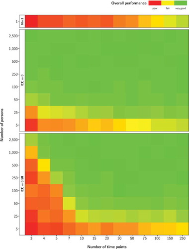
Figure 2. Overall performance (averaged over model parameters and performance criteria) depending on number of persons and number of time points for three scenarios (N = 1, ICC = 0, ICC = 0.50). The true auto-effect was a = –0.40 and the overall process mean was ${\mu }_{\mathrm{\infty }}^{\ast }$= 1

Results

Figure 2 shows the overall performance of the three scenarios: one person ($N$ = 1) at the top, multiple identical persons (ICC = 0) in the center, and multiple different persons (ICC = 0.50) at the bottom. The overall performance of the continuous-time model estimation for one person is rather poor for up to 100 time points. For 250 time points, the performance is good. For the ICC = 0 scenario, the performance becomes better with an increasing number of persons. For 25 persons, a good performance is already achieved for 15 time points; for 50 persons, performance is good when there are at least 3 time points. Such an $N$/$T$ compensation effect is present in the ICC = 0.50 scenario as well. However, the thresholds for a good performance are shifted to the upper right, indicated by more reddish cells in the lower left of the figure. This means that the performance worsens when the persons are not identical and a higher $N$/$T$ combination is needed to achieve good performance. Specifically, for our ICC = 0.50 scenario, performance starts to be satisfied for $N$/$T$ combinations of 2,500/3, 1,000/4, 500/5, 100/7, and 50/10. In these figures, we again see the compensation effect: To achieve the same good performance, we can lower the number of persons while raising the number of time points or, conversely, we can decrease the number of time points but then need to increase the number of persons.

Detailed results separately for performance criteria and model parameters are presented in Figures S1–S9 in the supplementary material. The convergence rate in the $N$ = 1 scenario is very good for 15 time points and more (Figure S1). Very good convergence rates were also achieved for essentially all $N$/$T$ combinations in the ICC = 0 scenario (Figure S4), whereas the thresholds for very good convergence in the ICC = 0.50 scenario are roughly on a diagonal line from upper-left to lower-right (Figure S7). Of all parameters, the auto-effect is the one that is worst recovered. For $N$ = 1, we observe very high relative bias for short time series and also for larger numbers of time points, relative bias is still not within the acceptable range (Figure S2). For five identical persons (ICC = 0), relative bias of the auto-effect reaches fair values for 50 time points or more. The relative bias is very good for all $T$ values for a number of persons of 50 or more (Figure S5). For different persons (ICC = 0.50), the threshold between poor and good performance is a roughly diagonal line from $N$ = 1,000/$T$ = 3 to $N$ = 25/$T$ = 15 (Figure S8). The picture changes for the coverage rates. Here, the auto-effect is among the best performing parameters, whereas the within-person process variance and the within-person variance at the first time point show worst coverage rates. For $N$ = 1, the coverage rates for the within-person process variance are poor for all $T$ (Figure S3). This gets better for larger $N$: starting from 250 time points, coverage rates are very good in the ICC = 0 scenario (Figure S6). For the ICC = 0.50 scenario, diagonal lines indicate the thresholds where poor performance turns into good performance (Figure S9).

In summary, we demonstrated that for a constant number of time points, performance increases with an increasing number of persons and, vice versa, for a constant number of persons, performance increases with an increasing number of time points. This is the $N$/$T$ compensation effect.

Additional simulations

In our simulation study, we used one set of true parameters. To investigate the dependence of results on true parameter values, we ran the simulation for the ICC = 0.50 scenario again, but this time varied the auto-effect $a$ ($-$1 vs. $-$0.25) and the process mean ${\mu }_{\mathrm{\infty }}^{\ast }$ ($-1$ vs. 3), yielding four parameter sets, set 1: $a=-1$/${\mu }_{\mathrm{\infty }}^{\ast }=-1$, set 2: $a=-1$/${\mu }_{\mathrm{\infty }}^{\ast }=3$, set 3: $a=-0.25$/${\mu }_{\mathrm{\infty }}^{\ast }=-1$, and set 4: $a=-0.25$/${\mu }_{\mathrm{\infty }}^{\ast }=3$. Procedures and analyses were as described above. Overall results for the four additional true parameter sets are shown in Figure 3. Detailed results are provided in the supplementary material (Figures S10–S21).

Figure 3. Overall performance (averaged over model parameters and performance criteria) depending on number of persons and number of time points for four true parameter sets (ICC = 0.50). For a high auto-effect (sets 3 and 4), bad overall performance occurred for some high N/T combinations (e.g., for 2,500/50 and 2,500/100). When using the true parameter values as starting values instead of the software’s default starting values, the performance was very good

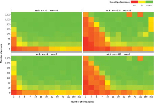
The results show that the performance indeed depends on the true parameter values. For a low auto-effect (left panels in Figure 3), estimation performance is much better than for a high auto-effect (right panels). Whereas performance is good for $N$/$T$ combinations of 100/4, 50/5, and 25/7 or higher for an auto-effect of $-1$, the picture changes for auto-effects of $-0.25$. Here, the thresholds for good performance are shifted to $N$/$T$ combinations of 2,500/4, 1000/5, and 500/7 or higher. With respect to the value of the process mean, there are only negligible performance differences.

Further, it can be seen that a high auto-effect (sets 3 and 4) is associated with bad overall performance for some high $N$/$T$ combinations, for example, for 2,500/50 and 2,500/100. Inspecting the detailed results (Figures S16–S21) suggests that this is mainly due to (very) low convergence rates and bad coverage rates. To explore the reason for this—in light of the $N$/$T$ compensation effect surprising—result, we reran the simulations for these problematic $N$/$T$ combinations, but used the true parameter values as starting values instead of the software’s default starting values. The performance then turned out to be very good (e.g., with convergence rates of 100%) and this again fits perfectly in the picture of the $N$/$T$ compensation effect. This outcome suggests that default starting values might be suboptimal for some situations.

Sample size recommendations

Although caution should be exercised when generalizing our findings beyond the conditions studied (see Discussion section), our findings are informative to guide study planning. We suggest to choose an $N$/$T$ combination with overall very good performance (green squares in Figures 2 and 3). Depending on what is more difficult to obtain, researchers could choose a certain limited $N$ and then compensate by increasing $T$, or choose a certain $T$ and compensate with larger $N$. In addition, they should have a more fine-grained look at Figures S1–S21 (in the supplementary material) and check whether the parameters of main interest show the desired performance. This is especially important the closer the $N$/$T$ combination comes to the red and yellow area. If accurate inferences for the parameters are imperative, we recommend to choose an $N$/$T$ combination for which the coverage rates for the parameters of interest are close to .95 (green or nearly green cells in Figures S3, S6, S9, S12, S15, S18, and S21). For data scenarios and models not studied in the present work, we caution to use the presented results only as a rule of thumb and recommend to additionally conduct tailored performance evaluations for the targeted scenarios and models. Further, we need to emphasize that default starting values might not always be the optimal choice, especially in situations known to cause convergence issues (e.g., when the auto-effect is high). In these situations, better starting values need to be chosen.

Discussion

In this article, we illustrated the $N$/$T$ compensation effect for longitudinal data analysis with continuous-time models. Smaller $T$ can be compensated with larger $N$, and vice versa, smaller $N$ can be compensated with larger $T$. Besides illustrating this compensation effect, we gave sample size recommendations to reach sufficient estimation performance for two popular continuous-time models. Therefore, this study joins in with numerous other studies on sample sizes that derive recommendations and exhibits, of course, similar limitations concerning generalizability.

As with all such studies, generalizing beyond the investigated conditions is difficult. Although we heavily varied and fully crossed our factors of interest ($N$ and $T$), we only considered a small number of sets of true parameter values, one assessment design, one estimation method/software, and two models. However, these factors were chosen as to reflect common use cases and frequently encountered situations in practice. Still, other research suggests that the factors we kept constant influence estimation performance as well. For instance, different performances of different models are one result in the work of Schultzberg and Muthén (2018) and the estimation performance of the autocorrelation parameter has been shown to depend on the estimation method (Krone et al., 2017) and the size and sign of the autocorrelation parameter (DeCarlo & Tryon, 1993; Solanas et al., 2010). In our simulations, we also found a dependency of the estimation performance on the value of the auto-effect, with a high auto-effect being associated with worse performance than a low auto-effect. Besides main effects, interaction effects of such factors are also possible and likely to occur. For example, the sign and strength of the autoregressive effect can affect the estimate of the process mean, particularly in short time series, with stronger positive autoregressive effects making it harder to estimate the mean (Schuurman et al., 2015).

Concerning generalizability to other models, we believe that the $N$/$T$ compensation effect is inherent and utilizable in all longitudinal two-level models that include distributional assumptions of individual parameters. This is because the distribution connects the individual parameters to one another and thus individual information informs distribution parameters which, in turn, informs individual parameters. Further, the extent to which estimation performance profits by adding persons likely depends on the similarity of the persons. We speculate that higher similarity (characterized by a lower ICC) enhances the information that is added in by an additional person and thus improves performance. Future research could investigate this effect.

The overall performance of the continuous-time model in the $N$ = 1 scenario was unsatisfactory for up to 100 time points and some parameters showed suboptimal performance on some criteria even for 250 time points. Thus, for our settings and model, the 50 time point rule of thumb from the $N$ = 1 discrete-time time-series literature does not apply and needs to be adjusted upward. This is in line with a finding by Yu (2012) that bias is much more pronounced in continuous-time models than in their discrete-time counterparts. More research on $N$ = 1 continuous-time modeling should be conducted to derive more accurate sample size requirements for these models.

Some coverage rates were quite bad, especially for low sample sizes. Reasons for this might lie in the way the confidence intervals were calculated (i.e., parameter $\pm$ 1.96$\cdot$$SE$). Thus, the assumption is that a parameter has a normal distribution. According to the central limit theorem (e.g., Box & Andersen, 1955), the parameter distribution rapidly converges to being asymptotically normally distributed with an increasing sample size for almost all parent distributions. For very small sample sizes, however, parameter distributions might deviate from the approximate normal distribution and therefore impair the performance of the confidence intervals. Further, confidence intervals are also sensitive to parameter bias with elevated bias being associated with worse coverage rates. We recommend to use only $N$/$T$ combinations for which the coverage rates for the parameters of interest are close to .95 (green or nearly green cells in Figures S3, S6, and S9). If smaller sample sizes are required, one might consult literature on the robustness of confidence intervals (e.g., Dorfman, 1994; Rao et al., 2003; Royall & Cumberland, 1985) or choose other approaches to obtain confidence intervals that do not depend on the normality assumption (e.g., Carpenter & Bithell, 2000; DiCiccio & Efron, 1996; Hu & Yang, 2013; Toth & Somorcik, 2017).

Further, our analysis model resembled the data-generating model. Negative effects of model misspecifications on estimation performance in autoregressive modeling contexts have been shown, for example, by Tanaka and Maekawa (1984) and Kunitomo and Yamamoto (1985). In sum, this leaves enough material for future research on sample size effects in continuous-time modeling. Such research is currently very sparse but, nonetheless, important because continuous-time models will most likely become even more prominent fueled by the rise of intensive longitudinal methods like ESM, EMA, and AA.

To conclude, we have clearly carved out the $N$/$T$ compensation effect in longitudinal data analysis and made some first tentative sample size recommendations for continuous-time modeling. We hope that this will prove useful in guiding researchers to better plan their intensive longitudinal studies in the future.

Acknowledgments

We acknowledge support by the Open Access Publication Fund of Humboldt-Universität zu Berlin.

Supplementary material

Supplemental data for this article can be accessed on the publisher’s website.

Notes

¹ We thank one anonymous reviewer for her or his elaborations.

² In line with Oud and Delsing (2010) and Hecht et al. (2019) we use the asterisk symbol * to denote discrete-time parameters that can be calculated from continuous-time parameters. In the present article, we limited ourselves to first-order continuous-time models with auto-effects, $a$, in the range ($-\mathrm{\infty },0$), which implies discrete-time autoregressive effects, $a_{{\mathrm{\Delta }}_{p-1}}^{\ast }$, in the range ($0,1$).

³ OpenMx sometimes outputs no standard errors even when the exit code is 0. We considered such analyses with missing standard errors (or highly inflated standard errors $>$ 1,000) for at least one parameter in the model as not converged as well because this points to estimation problems, and therefore such analyses are of the same low practical value for users as unconverged analyses. Still, with just 0.11% of all analyses, this was rarely the case.

⁴ Except for scenario 1 ($N$ = 1) in which the within-person variance at the first time point had to be constrained equal to the within-person process variance for identification reasons. As the true values of both variances were equal in the data generation, this constraint does not penalize the model performance in scenario 1.

References

- Arnau, J., & Bono, R. (2001). Autocorrelation and bias in short time series: An alternative estimator. Quality & Quantity, 35, 365–387. https://doi.org/10.1023/A:1012223430234
- Bisgaard, S., & Kulahci, M. (2011). Time series analysis and forecasting by example. Wiley.
- Box, G. E. P., & Andersen, S. L. (1955). Permutation theory in the derivation of robust criteria and the study of departures from assumption. Journal of the Royal Statistical Society, 17, 1–26. https://doi.org/10.1111/j.2517-6161.1955.tb00176.x
- Bulteel, K., Mestdagh, M., Tuerlinckx, F., & Ceulemans, E. (2018). VAR(1) based models do not always outpredict AR(1) models in typical psychological applications. Psychological Methods, 23, 740–756. https://doi.org/10.1037/met0000178
- Carpenter, J., & Bithell, J. (2000). Bootstrap confidence intervals: When, which, what? A practical guide for medical statisticians. Statistics in Medicine, 19, 1141–1164. https://doi.org/10.1002/(SICI)1097-0258(20000515)19:9<1141::AID-SIM479>3.0.CO;2-F
- DeCarlo, L. T., & Tryon, W. W. (1993). Estimating and testing autocorrelation with small samples: A comparison of the c-statistic to a modified estimator. Behaviour Research and Therapy, 31, 781–788. https://doi.org/10.1016/0005-7967(93)90009-J
- DiCiccio, T. J., & Efron, B. (1996). Bootstrap confidence intervals. Statistical Science, 11, 189–228. https://doi.org/10.1214/ss/1032280214
- Dorfman, A. H. (1994). A note on variance estimation for the regression estimator in double sampling. Journal of the American Statistical Association, 89, 137–140. https://doi.org/10.1080/01621459.1994.10476454
- Driver, C. C., Oud, J. H. L., & Voelkle, M. C. (2017). Continuous time structural equation modeling with R Package ctsem. Journal of Statistical Software, 77, 1–35. https://doi.org/10.18637/jss.v077.i05
- Driver, C. C., Oud, J. H. L., & Voelkle, M. C. (2019). ctsem: Continuous time structural equation modelling (Version 2.9.6) [Computer software]. https://cran.r-project.org/package=ctsem
- Driver, C. C., & Voelkle, M. C. (2018). Hierarchical Bayesian continuous time dynamic modeling. Psychological Methods, 23, 774–799. https://doi.org/10.1037/met0000168
- Hamaker, E. L., Kuiper, R. M., & Grasman, R. P. P. P. (2015). A critique of the cross-lagged panel model. Psychological Methods, 20, 102–116. https://doi.org/10.1037/a0038889
- Hecht, M., Hardt, K., Driver, C. C., & Voelkle, M. C. (2019). Bayesian continuous-time Rasch models. Psychological Methods, 24, 516–537. https://doi.org/10.1037/met0000205
- Hecht, M., & Voelkle, M. C. (2019). Continuous-time modeling in prevention research: An illustration. International Journal of Behavioral Development. Advance online publication. https://doi.org/10.1177/0165025419885026
- Hecht, M., & Zitzmann, S. (2020). A computationally more efficient Bayesian approach for estimating continuous-time models. Structural Equation Modeling. Advance online publication. https://doi.org/10.1080/10705511.2020.1719107
- Hu, Z., & Yang, R.-C. (2013). A new distribution-free approach to constructing the confidence region for multiple parameters. PLoS ONE, 8, 1–13. https://doi.org/10.1371/journal.pone.0081179
- Huitema, B. E., & McKean, J. W. (1991). Autocorrelation estimation and inference with small samples. Psychological Bulletin, 110, 291–304. https://doi.org/10.1037/0033-2909.110.2.291
- Huitema, B. E., & McKean, J. W. (1994). Reduced bias autocorrelation estimation: Three jackknife methods. Educational and Psychological Measurement, 54, 654–665. https://doi.org/10.1177/0013164494054003008
- Jebb, A. T., Tay, L., Wang, W., & Huang, Q. (2015). Time series analysis for psychological research: Examining and forecasting change. Frontiers in Psychology, 6, 1–24. https://doi.org/10.3389/fpsyg.2015.00727
- Kearney, M. W. (2017). Cross-lagged panel analysis. In M. R. Allen (Ed.), The SAGE encyclopedia of communication research methods (pp. 312–314). SAGE.
- Krone, T., Albers, C. J., & Timmerman, M. E. (2017). A comparative simulation study of AR(1) estimators in short time series. Quality & Quantity, 51, 1–21. https://doi.org/10.1007/s11135-015-0290-1
- Kunitomo, N., & Yamamoto, T. (1985). Properties of predictors in misspecified autoregressive time series models. Journal of the American Statistical Association, 80, 941–950. https://doi.org/10.1080/01621459.1985.10478208
- McCleary, R., Hay, R. A., Meidinger, E. E., & McDowall, D. (1980). Applied time series analysis for the social sciences. SAGE.
- Muthén, L. K., & Muthén, B. O. (2002). How to use a Monte Carlo study to decide on sample size and determine power. Structural Equation Modeling, 9, 599–620. https://doi.org/10.1207/S15328007SEM0904_8
- Neale, M. C., Hunter, M. D., Pritikin, J. N., Zahery, M., Brick, T. R., Kirkpatrick, R. M., Estabrook, R., Bates, T. C., Maes, H. H., & Boker, S. M. (2016). OpenMx 2.0: Extended structural equation and statistical modeling. Psychometrika, 81, 535–549. https://doi.org/10.1007/s11336-014-9435-8
- Oud, J. H. L., & Delsing, M. J. M. H. (2010). Continuous time modeling of panel data by means of SEM. In K. van Montfort, J. H. L. Oud, & A. Satorra (Eds.), Longitudinal research with latent variables (pp. 201–244). Springer.
- Oud, J. H. L., Voelkle, M. C., & Driver, C. C. (2018). First- and higher-order continuous time models for arbitrary N using SEM. In K. van Montfort, J. H. L. Oud, & M. C. Voelkle (Eds.), Continuous time modeling in the behavioral and related sciences (pp. 1–26). Springer.
- Poole, M. S., McPhee, R. D., & Canary, D. J. (2002). Hypothesis testing and modeling perspectives on inquiry. In M. L. Knapp & J. A. Daly (Eds.), Handbook of interpersonal communication (3rd ed., pp. 23–72). SAGE.
- R Core Team. (2019). R: A language and environment for statistical computing. (Version 3.6.1) [Computer software]. R Foundation for Statistical Computing. https://www.r-project.org
- Rao, J. N. K., Jocelyn, W., & Hidiroglou, M. A. (2003). Confidence interval coverage properties for regression estimators in uni-phase and two-phase sampling. Journal of Official Statistics, 19, 17–30. https://www.scb.se/contentassets/ca21efb41fee47d293bbee5bf7be7fb3/confidence-interval-coverage-properties-for-regression-estimators-in-uni-phase-and-two-phase-sampling.pdf
- Royall, R. M., & Cumberland, W. G. (1985). Conditional coverage properties of finite population confidence intervals. Journal of the American Statistical Association, 80, 355–359. https://doi.org/10.1080/01621459.1985.10478122
- Schultzberg, M., & Muthén, B. (2018). Number of subjects and time points needed for multilevel time-series analysis: A simulation study of dynamic structural equation modeling. Structural Equation Modeling, 25, 495–515. https://doi.org/10.1080/10705511.2017.1392862
- Schuurman, N. K., Houtveen, J. H., & Hamaker, E. L. (2015). Incorporating measurement error in n = 1 psychological autoregressive modeling. Frontiers in Psychology, 6, 1–15. https://doi.org/10.3389/fpsyg.2015.01038
- Selig, J. P., & Little, T. D. (2012). Autoregressive and cross-lagged panel analysis for longitudinal data. In B. Laursen, T. D. Little, & N. A. Card (Eds.), Handbook of developmental research methods (pp. 265–278). The Guilford Press.
- Solanas, A., Manolov, R., & Sierra, V. (2010). Lag-one autocorrelation in short series: Estimation and hypotheses testing. Psicológica, 31, 357–381. https://www.uv.es/psicologica/articulos2.10/9SOLANAS.pdf
- Tanaka, K., & Maekawa, K. (1984). The sampling distributions of the predictor for an autoregressive model under misspecifications. Journal of Econometrics, 25, 327–351. https://doi.org/10.1016/0304-4076(84)90005-8
- Toth, R., & Somorcik, J. (2017). On a non-parametric confidence interval for the regression slope. METRON, 75, 359–369. https://doi.org/10.1007/s40300-017-0109-z
- Voelkle, M. C., Oud, J. H. L., Davidov, E., & Schmidt, P. (2012). An SEM approach to continuous time modeling of panel data: Relating authoritarianism and anomia. Psychological Methods, 17, 176–192. https://doi.org/10.1037/a0027543
- Warner, R. M. (1998). Spectral analysis of time-series data. Guilford Press.
- Yu, J. (2012). Bias in the estimation of the mean reversion parameter in continuous time models. Journal of Econometrics, 169, 114–122. https://doi.org/10.1016/j.jeconom.2012.01.004