Three Extensions of the Random Intercept Cross-Lagged Panel Model

ABSTRACT

The random intercept cross-lagged panel model (RI-CLPM) is rapidly gaining popularity in psychology and related fields as a structural equation modeling (SEM) approach to longitudinal data. It decomposes observed scores into within-unit dynamics and stable, between-unit differences. This paper discusses three extensions of the RI-CLPM that researchers may be interested in, but are unsure of how to accomplish: (a) including stable, person-level characteristics as predictors and/or outcomes; (b) specifying a multiple-group version; and (c) including multiple indicators. For each extension, we discuss which models need to be run in order to investigate underlying assumptions, and we demonstrate the various modeling options using a motivating example. We provide fully annotated code for lavaan (R-package) and Mplus on an accompanying website.

KEYWORDS:

• Random-Intercept Cross-Lagged Panel Model
• panel data
• within-person dynamics
• longitudinal modeling

The random intercept cross-lagged panel model (RI-CLPM) proposed by Hamaker et al. (2015) is an extension of the traditional cross-lagged panel model (CLPM). It was introduced to account for stable, trait-like differences between units (e.g., individuals, dyads, families, etc.), such that the lagged relations pertain exclusively to within-unit fluctuations.¹ The idea that we should decompose longitudinal data into stable, between-unit differences versus temporal, within-unit dynamics is closely linked to the multilevel literature on cluster-mean centering (Bolger & Laurenceau, 2013; Enders & Tofighi, 2007; Kievit et al., 2013; Kreft et al., 1995; Mundlak, 1978; Neuhaus & Kalbfleisch, 1998; Nezlek, 2001; Raudenbush & Bryk, 2002; Snijders & Bosker, 2012). Alternatively, it can also be linked to the discussion in panel research on the need to account for unobserved heterogeneity in longitudinal data (Allison et al., 2017; Bianconcini & Bollen, 2018; Bollen & Brand, 2010; Bou & Satorra, 2018; Finkel, 1995; Hamaker & Muthén, 2020; Liker et al., 1985; Ousey et al., 2011; Wooldridge, 2002, 2013). A detailed discussion of how other common panel models account for unobserved heterogeneity (as well as for measurement error and developmental trajectories) is provided by Usami et al. (2019), Zyphur et al. (2019a), and Zyphur et al. (2019b).

The appeal of the RI-CLPM can be attributed to three factors. First, the basic idea that one needs to decompose the observed variance into two sources resonates with a concern many researchers have had about the traditional CLPM (Keijsers, 2016). In fact, there have been numerous other proposals aiming to do exactly this (e.g., Allison et al., 2017; Bianconcini & Bollen, 2018; Kenny & Zautra, 1995; Ormel et al., 2002; Ormel & Schaufeli, 1991; Ousey et al., 2011). Second, the model can be applied if one has three occasions of data or more, using any structural equation modeling (SEM) software package, which makes the approach broadly applicable and easy to implement. Third, the RI-CLPM tends to fit empirical data (much) better than the traditional CLPM, as is corroborated by empirical work of, for instance, Borghuis et al. (2020), R. A. Burns et al. (2019), and Keijsers (2016). The second-order lagged relations that are often needed to get a CLPM to have an acceptable fit are typically not needed in the RI-CLPM, because the long-run, trait-like stability is now captured by the random intercepts instead of by the second-order lagged relations.

Given the growing popularity of the RI-CLPM, it is not surprising that researchers are interested in how they can adapt the basic model to accommodate their particular data and research interests. Examples of this can be found in the Mplus Discussion Board thread on the RI-CLPM,² the Lavaan forum,³ and RI-CLPM-related posts on SEMNET.⁴ Some of the most frequently asked questions are how to extend the model by (a) including person-level characteristics (e.g., social-economic status, personality factors, age, health) as a predictor or outcome variable, (b) performing a multiple-group version of the model to investigate whether lagged relationships are different across groups, and (c) using multiple indicators for latent variables in the model. The purpose of the current paper is to elaborate on these extensions and help researchers navigate the different modeling options and assumptions.

This paper is organized as follows. In the first section, we begin with presenting the RI-CLPM, and discuss how it is related to the traditional CLPM. In the following three sections we discuss the three different extensions described above and we will focus on the modeling options available. To facilitate the explanation of the model and its results we will use a motivating example about the reciprocal effects of sleep problems and anxiety in young adolescents based on Narmandakh et al. (2020). Furthermore, to allow the reader to obtain hands-on experience with this modeling approach, we provide a simulated data set of our motivating example, as well as annotated lavaan code and Mplus syntax (see: jeroendmulder.github.io/RI-CLPM).

The RI-CLPM and the traditional CLPM

Below, we begin with discussing how the RI-CLPM is build up. Subsequently, we discuss diverse constraints over time that can be imposed or relaxed. We end by briefly discussing how this model is related to the traditional CLPM. While the terminology used here is clearly inspired by the multilevel literature (where there is a between-cluster level and a within-cluster level), the RI-CLPM is estimated in wide-format using structural equation modeling (SEM), rather than in long-format with multilevel modeling. Throughout we make use of a simulated data set that was motivated by Narmandakh et al. (2020). In their study, five waves of data were obtained from 1189 adolescents on their sleep problems and anxiety during the past 15 years.

Building up the basic RI-CLPM

To fit an RI-CLPM, we need to decompose the observed scores into three components: grand means, stable between components, and fluctuating within components. This decomposition is illustrated in the upper panel of Figure 1. Let $S_{it}$ and $A_{it}$ represent the observed scores on sleep problems and anxiety for person $i$ at occasion $t$, respectively. The first components are the grand means, which are the means over all units per occasion $t$, and represented by ${\mu }_t$ for sleep problems and ${\pi }_t$ for anxiety. These grand means may be time-varying, or may be fixed to be invariant over time. Second, the between components, indicated by the letter $B$, are the random intercepts: $B{S}_i$ for sleep problems and $B{A}_i$ for anxiety. They capture a unit’s time-invariant deviation from the grand means and thus represent the stable differences between units. The random intercepts are specified in SEM software by creating a latent variable with the repeated measures as its indicators, and fixing all the factor loadings to 1. Third, the within components, indicated by the letter $W$, are the differences between a units observed measurements and the unit’s expected score based on the grand means and its random intercepts. $W{S}_{it}$ and $W{A}_{it}$ thus represent the within components of sleep problems and anxiety, respectively. We create these components in SEM software by specifying a latent variable for each measurement and constraining its measurement error variances to 0. As a result, we have $S_{it}={\mu }_t+B{S}_i+W{S}_{it}$ and $A_{it}={\pi }_t+B{A}_i+W{A}_{it}$.

Figure 1. Graphic representations of the random intercept cross-lagged panel model (RI-CLPM) and the traditional cross-lagged panel model (CLPM). $S_{it}$ denotes the observed sleep problems and $A_{it}$ denotes the observed anxiety of unit $i$ at occasion $t$

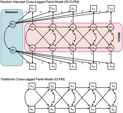
Next, we specify the structural relations between the within components. The autoregressive effects (i.e., ${\alpha }_t$ from $W{S}_{it-1}$ to $W{S}_{it}$ and ${\delta }_t$ from $W{A}_{it-1}$ to $W{A}_{it}$) represent the within-person carry-over effects. If ${\alpha }_t$ is positive, this implies that an individual who experiences elevated sleep problems relative to his/her own expected score, is likely to experience elevated sleep problems relative to his/her own expected score at the next occasion as well. The same logic applies to the interpretation of ${\delta }_t$. For this reason, the within-person autoregressive effects are sometimes referred to as inertia (i.e., the tendency to not move; see Suls et al., 1998). The cross-lagged effects in the model represent the spill-over of the state in one domain into the state of another domain. Here, ${\beta }_t$ represents the effect of $W{S}_{it-1}$ to $W{A}_{it}$ and ${\gamma }_t$ the effect of $W{A}_{it-1}$ to $W{S}_{it}$. A positive ${\beta }_t$ implies that a positive (negative) deviation from an individual’s expected level of sleep problems will likely be followed by a positive (negative) deviation in the individual’s expected level of anxiety at the next occasion in the same direction. The same logic applies to ${\gamma }_t$.

Finally, we need to include covariances for both the within and between components of the model. For the within part, we specify that the components at occasion 1 and the within-person residuals at all subsequent occasions are correlated within each occasion. For the between part, we specify that the random intercepts are correlated. We are not including covariances between the within-person components at the first occasion and the random intercepts because typically the observations have started at an arbitrary time point in an ongoing process and there is no reason to assume that the within components at the first occasion are correlated to the random intercepts.⁵

Applying this model to our simulated example data, we find that both random intercepts have significant variance, which implies that there are stable, trait-like differences between persons on sleep problems and anxiety. Moreover, we find a significant positive covariance between the random intercepts of $.01$ with $SE=.001$ (the correlation is $.59$, $SE=.050$), suggesting that individuals who have more sleep problems, in general, are also more anxious in general.

If, in contrast to our findings here, the variance of a random intercept does not significantly differ from 0, this means that there are little to no stable between-unit differences, and that each unit fluctuates around the same grand means over time. Including a random intercept in the model can then be regarded as redundant; such a model would be too complex for the data. In that case, one can choose to either fix the non-significant variance (and all the covariances between this random intercept and the other intercepts) to 0, or simply remove the random intercept from the model and include lagged-relations between the observed variables instead of between the within-unit components. These two solutions are statistically equivalent and will lead to the same lagged-parameter estimates and model fit. Note that it is possible to have a model in which one variable needs to be decomposed into a between-unit and a within-unit part, while the other variable does not require such a decomposition.

Looking at the within part of the model we find the following standardized autoregressive effects for sleep problems, ${\alpha }_2=.29$ ($SE=.034$), ${\alpha }_3=.24$ ($SE=.036$), ${\alpha }_4=.27$ ($SE=.036$), ${\alpha }_5=.29$ ($SE=.035$), and for anxiety, ${\delta }_2=.004$ ($SE=.045$), ${\delta }_3=.25$ ($SE=.036$), ${\delta }_4=.29$ ($SE=.033$), ${\delta }_5=.40$ ($SE=.030$). There are also significant cross-lagged effects of sleep problems to anxiety, ${\beta }_2=.15$ ($SE=.039$), ${\beta }_3=.10$ ($SE=.035$), ${\beta }_4=.11$ ($SE=.034$), ${\beta }_5=.08$ ($SE=.031$), which means that individuals with relatively little sleep problems (relative to an individual’s own mean) will likely experience relatively little anxiety at the next occasion. However, none of the cross-lagged effects from anxiety to sleep problems are significant, which means that an individual’s temporary elevated or damped amount of sleep problems does not depend on that individual’s temporary level of anxiety at the previous occasion.

Imposing constraints over time

To test specific hypotheses, researchers can decide to impose constraints on the model and test the tenability of these constraints. This can be done by comparing the fit of a (nested) model with constraints to the fit of the more general model using a chi-square difference test ($\mathrm{\Delta }{\chi }^2$); if the constrained model fits the data significantly worse, the imposed constraints are untenable. Alternatively, one can use the AIC or BIC as measures of model fit to compare both non-nested and nested models, where the model with the lower AIC or BIC should be preferred.

The use of the chi-square difference test is wide-spread in the SEM community, but a few cautionary notes are in order. First, parameters should only be constrained if the constraints make theoretical sense, and not solely because it leads to a more parsimonious model. Second, failing to detect a significantly worse fitting model in a sequence of chi-square difference tests does not imply that the constrained model represents the population well. It is possible that the unconstrained base model was misspecified in the first place and this misspecification will carry on into the constrained model. In that case, the chi-square difference test is unable to control for Type I error rates and retain adequate power (Yuan & Bentler, 2004). Careful consideration should always be given to the fit of the models themselves by looking at a variety of model fit indices.

In the RI-CLPM, there are several constraints over time that can be added. We discuss two common ones here. First, we may consider testing if the lagged regression coefficients are time-invariant. This can be done by comparing the fit of a model with constrained regression coefficients (over time), with the fit of a model where these parameters are freely estimated (i.e., the unconstrained model). If this chi-square difference test is non-significant, this implies the constraints are tenable and the dynamics of the process are time-invariant. If the constraints are not tenable, this could be indicative of some kind of developmental process taking place during the time span covered by the study.

In this context, it is important to realize that the lagged regression coefficients depend critically on the time interval between the repeated measures. Hence, constraining the lagged parameters to be invariant across consecutive waves only makes sense when the time interval between the occasions is (approximately) equal (Gollob & Reichardt, 1987; Kuiper & Ryan, 2018; Voelkle et al., 2012). If the time intervals between subsequent occasions vary, we are estimating different autoregressive and cross-lagged effects between each pair of adjacent measurements. In such a situation, constraining the lagged regression coefficients leads to an uninterpretable blend of different lagged relationships. Furthermore, even when the lagged parameters are invariant over time, this will typically not be true for the standardized lagged parameters, because these are a function of the within-unit variance of the predictor and the within-unit variance of the outcome. As these variances are typically not (constrained to be) equal across the occasions (which is complicated due to the recursiveness in the model), the standardized lagged parameters can differ even if the unstandardized lagged parameters are constrained to be the same (Hamaker et al., 2015).

To test if the lagged relations in our sleep problems and anxiety example are invariant over time, we fit a model with constrained lagged regression coefficients and find ${\chi }^2=90.97$ with 33 degrees of freedom. The unconstrained model (the basic RI-CLPM fitted before) has ${\chi }^2=25.81$ with 21 degrees of freedom. The chi-square difference test of these two nested models is thus $\mathrm{\Delta }{\chi }^2(12)=65.16$, with $p<.001$. Hence, constraining the lagged effects to be the same over time results in a significantly worse model fit. We, therefore, conclude that the constraints are untenable and that there appears to be a change in within-person dynamics over time. Upon closer inspection of the autoregressive effects of anxiety ${\delta }_t$ in the unconstrained model, this makes sense: These estimates increase with each subsequent occasion, from $.004$ to $.40$.

Second, we may investigate whether the grand means, ${\mu }_t$ and ${\pi }_t$, are invariant over time. This can be done by constraining the means to be the same across occasions and performing the chi-square difference test to determine whether this constraint can be imposed. If this is the case, this implies we are dealing with a construct that is stable at the population level for the duration of the study. In contrast, if the grand means cannot be constrained to be invariant over time, this implies that on average there is some change in this variable over time, which may reflect some occasion-specific effect, or a developmental trend. By allowing the means to freely vary over time, we account for such average changes over time. In our example a comparison of the constrained and the unconstrained models yields a chi-square difference test of $\mathrm{\Delta }{\chi }^2(8)=434.20$, $p<.001$, which implies that the constraints are untenable and that the grand means vary over time.

Alternatively, one can choose to relax; instead, of impose, constraints over time to allow for a more flexible and better fitting model. The RI-CLPM is based on the assumption that the random intercepts have the exact same influence on the observed variables at each occasion, which is reflected by the factor loadings that are all constrained to be 1 over time. However, researchers may want to test this, which can be done by comparing the model with these constrained factor loadings to a model in which the factor loadings are estimated freely; the latter model implies that there are stable, trait-like differences between individuals, but the size of these differences can change over time. The between components are then no longer random intercepts, but can be interpreted as traits. To fit a model with freely estimated factor loadings, at least four occasions of data are needed; in contrast, with the fixed factor loadings, the model is already identified with only three waves of data.

Relatedness to the traditional CLPM

If we constrain the variances of all random intercepts (and their covariance) in the RI-CLPM to zero, we obtain a model that is nested under the RI-CLPM, and no longer accounts for stable between-unit differences. This model is actually statistically equivalent to the traditional CLPM (represented in the bottom panel of Figure 1), which implies that we can compare these two models using a chi-square difference test.⁶

In comparison to the traditional CLPM, the RI-CLPM often leads to autoregressive parameters that are closer to zero with larger standard errors. As a result, the autoregressive parameters that are significantly different from zero in the CLPM, may not be significant in the RI-CLPM. This has led some to speculate that the reliability of the within-unit components in the RI-CLPM is low. However, it is important to realize that the autoregressive parameters represent quite different phenomena in these two models. In the traditional CLPM, the autoregressive parameter captures the stability of the rank-order of individuals from one occasion to the next. It is closely related to the idea of test–retest reliability, which uses the autocorrelation as a measure of the reliability of a time-invariant, trait-like construct. In the RI-CLPM however, the trait-like features are captured by the random intercepts, such that the autoregressive parameters are not there to capture rank-order stability due to a trait, but to account for additional moment-to-moment stability (i.e., inertia or carry-over) of the within-unit fluctuations over time. Hence, in the RI-CLPM, the autoregressive parameters should not be considered as measures of reliability, because reliability and stability do not coincide for state-like concepts (Hertzog & Nesselroade, 1987).

With respect to the cross-lagged parameters, there can be a number of differences between the two models. As discussed in the original paper by Hamaker et al. (2015), we may find cross-lagged paths in the CLPM that seize to exist in the RI-CLPM or vice versa, the standardized absolute values of the cross-lagged parameters may lead to a different ordering, and even the sign of a cross-lagged path may change. The latter result has been corroborated in empirical research by Dietvorst et al. (2018). The extent to which results change depends on various factors, including the relative contributions of the within-unit and the between-unit components to the total variance. For instance, when the relative contribution of the between-unit components is small, the lagged parameters of the two models will be quite similar.

Furthermore, Dormann and Griffin (2015) have recently argued that many of our conventional panel studies are probably based on intervals that are too large to capture the underlying within-unit dynamic relationships. Instead, the lagged effects that are found with the CLPM might result from stable between-unit differences rather than dynamic within-unit relations. This would imply that many of the significant results that are obtained with the CLPM, will not be replicated when using an RI-CLPM because the stable between-unit differences, captured by first and second-order lagged effects in the CLPM, are now captured by the random intercepts in the RI-CLPM (Keijsers, 2016). Yet, the extent to which the results from the traditional CLPM and the RI-CLPM will differ cannot be predicted; the discrepancy or similarity will have to be established empirically through fitting both models to the data and comparing the results.

Conclusion

We have provided a brief introduction to the modeling and reasoning behind the RI-CLPM, and illustrated the basic steps researchers should consider when using this modeling approach. For more details on how this model is related to other longitudinal SEM approaches, the reader is referred to Usami et al. (2019) and Hamaker et al. (2015). In the remainder of this paper, we discuss several extensions of the basic RI-CLPM.

Extension 1: Including time-invariant predictors and outcomes

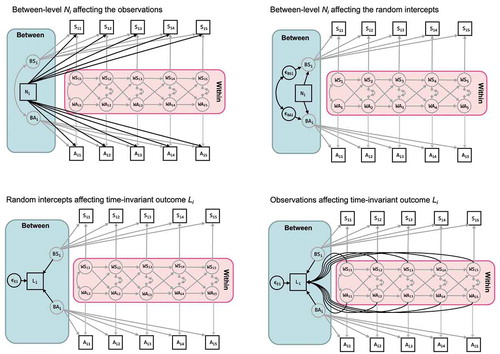
If we have obtained certain time-invariant person characteristics prior to the repeated measures — such as social-economic status, personality, age, or gender — we may want to include these as predictors in the RI-CLPM. A question that arises in this context is whether these variables should be used to predict the observed variables or the random intercepts. These two options for an observed predictor variable are represented in the top row of Figure 2. In this section, we discuss both options in more detail and show how they are related. Additionally, we discuss how one may include time-invariant distal outcomes — such as later educational level, life satisfaction, or depression — in the RI-CLPM.

Figure 2. Two options for including a between-level predictor: In the top left, $N_i$ influences the observed variables directly; in the top right, this occurs indirectly through the random intercepts. The model in the top right is nested under the model in the top left (fixing the regression coefficients to be identical over time results in a version that is equivalent to the model on the right). Also, two options for including a between-level outcome: In the lower-left, $L_i$ is explained by the random intercepts which includes only between variance; in the lower right, panel the distal outcome is regressed on both the random intercepts and the within components such that we use both between- and within-level variance to predict $L_i$. These two models are not nested

It is important to realize that adding variables to our model changes the covariance structure that is being analyzed, and in SEM we can only compare models that are based on the same set of variables. As a result, a model with a time-invariant predictor is not comparable to a model that excludes it. Likewise, it is possible to have a well-fitting model, which is then extended with a predictor that proves significant, while this extended model no longer fits. The reason for this is that the two models are based on different covariance and mean structures.

Including a time-invariant predictor

Let $N_i$ be a measure of an individual’s neuroticism, which we want to include as a predictor of the observed variables $S_{it}$ and $A_{it}$, as represented in the top left panel of Figure 2. This allows the effect of neuroticism on sleep problems and the effect of neuroticism on anxiety to be different at each occasion $t$. In the particular case that $N_i$ is a dummy variable (as in our example here), the regression coefficients can be interpreted as mean differences between the group represented by the dummy variable, and the reference group (represented by zero scores on all dummy variables). We include a dummy for individuals who are high on neuroticism, which results in significant positive effects of neuroticism on both sleep problems and anxiety. This suggests that highly neurotic adolescents experience more sleep problems and have more anxiety symptoms than adolescents in the low-neuroticism group, and this result holds for all occasions. As a restricted version of this model, we can constrain the effects of neuroticism on sleep problems and anxiety to be the same at each occasion $t$. Because these models are nested, we can perform a chi-square difference test to determine whether these constraints can be imposed.

The latter constrained model is statistically equivalent to a model in which the random intercepts, rather than the observed variables, are regressed on $N_i$ (represented in the top right panel of Figure 2). This is only the case however if the factor loadings of the random intercepts are all fixed at 1 like in the basic RI-CLPM discussed before. Imposing the constraints leads to a chi-square difference test of $\mathrm{\Delta }{\chi }^2(8)=8.91$ with $p=.350$, which implies that the effects of neuroticism on the random intercepts of sleep problems and anxiety are time-invariant: the estimated standardized effects are $.27$ ($SE=.040$) and $.24$ ($SE=.035$), respectively. Therefore, we conclude that high-neuroticism adolescents experience more sleep problems and anxiety in general than low-neuroticism individuals.

Including a time-invariant outcome

Suppose we have measured later life satisfaction $L_i$ after the repeated measures, and we want to predict this using sleep problems and anxiety. We can do this by regressing $L_i$ either on the random intercepts $B{S}_i$ and $B{A}_i$, the within-person fluctuations $W{S}_{it}$ and $W{A}_{it}$, or on the observed variables $S_{it}$ and $A_{it}$. The first two options are represented in the bottom panels of Figure 2. From a substantive point of view, regressing life satisfaction on the random intercepts implies that temporal within-person fluctuations in sleep problems and anxiety, $W{S}_{it}$ and $W{A}_{it}$, are not informative for predicting later life satisfaction as the random intercepts only contain stable between person information. This assumption is defendable as a later educational level is a time-invariant outcome and therefore belongs to the between part of the model.

Alternatively, one can decide to regress the outcome on both the random intercepts and the temporal deviations. The regression on the random intercepts then represents the predictive value of between components net the predictive value of the within part, and the regression on the temporal deviations represents the predictive value of the within components net the predictive value of the between part. As such, we separate the total predictive power of our variables into a uniquely between and uniquely within component. The decision to use only between-unit variance, or both within- and between-unit variance to predict the outcome, should ideally be based on theoretical grounds. However, if this is something that the researcher explicitly wants to test one can fit the above two models and compare them using a chi-square difference test where the model with the outcome regressed on the random intercepts is nested under the current model.

A third option is regressing $L_i$ on the observed variables, which implies that one assumes that both between-person variance that comes from the random intercepts, and temporary, within-person variance that comes from the within-person components, are informative about later depression. However, we find this modeling option less defendable as it again blends stable between-effects and fluctuating within-effects, an issue that the RI-CLPM aims to address in the first place. By regressing the outcome on both the within-components and between-components separately, researchers can check if within variance provides additional predictive value over the between variance.

Including both a predictor and outcome

We can also consider including both neuroticism as a predictor and later life satisfaction as an outcome at the between level. If this is all specified at the between level, this implies neuroticism has an indirect effect on life satisfaction through the random intercepts and this can be considered as a case of mediation at the between level. We can also include the direct effect of neuroticism on life satisfaction to allow for partial mediation.

Extension 2: The multiple group RI-CLPM

In the previous section, we used a dummy variable for neuroticism as a predictor in our model, which allowed us to investigate whether there are mean differences between the group high on neuroticism, and the group low on neuroticism. Alternatively, one can use such a categorical variable as a grouping variable in multiple group analysis (e.g., Vangeel et al., 2018; Van Lissa, Keizer, Lier, Van Meeus, and Branje, 2019). This approach implies that not only the means can differ across the groups (as is the case when including dummy variables as predictors of the random intercepts or the observed variables, as described in the previous section), but also the lagged regression coefficients, the (residual) variances, and the (residual) covariances.

Group differences in lagged regression coefficients can be thought of as moderation or interaction effects, and may, therefore, be of specific interest to researchers. This can be investigated by comparing a multiple group version of the RI-CLPM in which there are no constraints across the groups, with a model in which the lagged regression coefficients are constrained to be identical across the groups. If the chi-square difference test indicates that this constraint cannot be imposed, this implies that (some of) the lagged coefficients differ across the groups: The lagged effects of the variables on each other depend on the level of the grouping variable. In contrast, when the equality constraints on the lagged parameters across the groups hold, this implies there is no moderation effect. However, note again that the constraints only imply that the raw coefficients are invariant across groups; the standardized lagged effects may still differ across the groups in case the variances differ across groups.

To test if the reciprocal effects between sleep problems and anxiety are the same for those high in neuroticism versus those low in neuroticism, we perform a multiple group analysis. First, we fit a multiple group RI-CLPM without constraints across the groups and find ${\chi }^2(42)=45.64$. Subsequently, we fit a model in which lagged parameters are invariant across groups and find ${\chi }^2(58)=54.80$. The chi-square difference test of these two nested models yields $\mathrm{\Delta }{\chi }^2(16)=9.162$, $p=.907$, which implies that imposing the constraints is tenable: The lagged effects for individuals with different levels of neuroticism appear to be the same.

Extension 3: The multiple indicator RI-CLPM

Another way in which researchers may wish to extend the RI-CLPM is by including multiple indicators for each of the constructs, while formulating the dynamics over time between the latent variables. There are two ways in which this can be done. First, a random intercept can be included for each indicator, as shown in the top panel of Figure 3, and these random intercepts are allowed to be correlated with each other. In addition, a common factor of the multiple indicators is included per occasion to capture the common within-unit variability over time. Second, the random intercepts can be included at the latent level as shown in the bottom panel of Figure 3 (e.g., see Seddig, 2020). There is a common factor for each construct at each occasion, which is then being further decomposed into a time-invariant part captured by the random intercept, and a time-varying part that is used to model the within-unit dynamics. These two approaches are nested with the second being a special case of the first.

Figure 3. Two options for incorporating multiple indicators in a RI-CLPM. Top panel shows a model with indicator-specific random intercepts that capture trait-like differences between units, and occasion-specific factors that capture the within-unit dynamics. Bottom panel shows a model in which there is a latent variable per occasion, which contains a trait-like part that is captured by the higher-order random intercepts, and a state-like part that is used to capture the dynamics over time

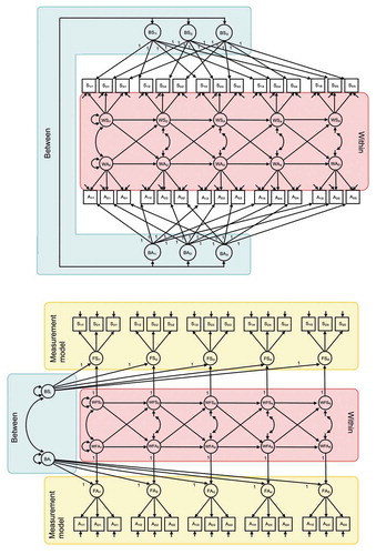
To allow for a meaningful comparison of factors over time, the factor loadings should be time-invariant, such that there is (at least) weak factorial invariance over time (Meredith, 1993; Millsap, 2011). If we are unable to establish this invariance, it implies that the constructs that we try to measure are interpreted differently over time, and it is difficult to make meaningful comparisons between the constructs measured at different occasions. Below we discuss the sequence of models that needs to be considered to establish longitudinal measurement invariance, and detail how the decomposition into within-unit and between-unit variance can be obtained in the context of multiple indicators.

In the first model, we decompose each observed variable into two parts: A stable, between-unit part, and a time-varying, within-unit part that indicators have in common (see Figure 3). Thus, if we use three indicators to measure sleep problems, $S_{1it}$, $S_{2it}$, and $S_{3it}$, and three indicators to measure anxiety, $A_{1it}$, $A_{2it}$, and $A_{3it}$, we specify six random intercepts to capture the trait-like part of each indicator. In addition, since we have five measurement occasions, we need to specify five within-unit components for sleep problems, $W{S}_{it}$, and five for anxiety, $W{A}_{it}$, that capture the common state-like part at each occasion. Moreover, we allow there to be an occasion- and indicator-specific residual, that captures what each observed variable does not share with itself at other occasions or with the other variables within the same occasion, thus capturing measurement error. At the latent within-unit level, we specify the dynamic model. Furthermore, we allow the within-person factors at the first occasion, and their residuals at subsequent occasions to be correlated within each occasion. The six random intercepts are allowed to be freely correlated with each other. In this model there are no constraints on the factor loadings over time for the within-unit factors; hence, this can be considered a model for configural invariance.

In the second model, we constrain the factor loadings to be invariant over time. This model is nested under the previous model, such that we can do a chi-square difference test. Fitting both models to our example data and comparing them yields $\mathrm{\Delta }{\chi }^2(16)=10.12$, $p=.861$ and we conclude that the model with invariant factor loadings over time does not fit significantly worse. Therefore, we can assume weak factorial invariance holds. In contrast, a significant test implies that the factor loadings cannot be constrained over time, making further comparisons between the latent variables problematic or even impossible. There are however two ways of dealing with this problem (Lek et al., 2018; Seddig & Leitgöb, 2018). First, by checking the modification indices, we can determine whether there is a specific factor loading at a particular measurement occasion that wildly deviates from the other factor loadings that it is constrained to be equal to. In such a case, researchers can choose to freely estimate this particular factor loading, resulting in a model that is based on partial measurement invariance. The model then accounts for a large measurement difference associated with a particular indicator while retaining weak measurement invariance for the rest of the indicators. Second, recently researchers have argued that the traditional concepts and tests of measurement invariance are too strict for small measurement differences. They advocate the use of approximate measurement invariance which allows for these minor differences through the use of priors in Bayesian estimation procedures. An introduction to the concept of approximate measurement invariance can found in Van de Schoot et al. (2013).

Assuming that weak factorial invariance holds, we can proceed with the third model and test whether strong factorial invariance holds. To this end, we specify a model in which we constrain the intercepts of the observed variables over time to be invariant, and estimate the latent means from the second occasion onward.⁷ Again, this model is nested under the previous model, such that a chi-square difference test can be performed to see whether the constraints hold. Applying this test to our example data, we find $\mathrm{\Delta }{\chi }^2(16)=21.64$, $p=.155$, which means we can assume that strong factorial invariance holds over time. In contrast, a significant chi-square difference test would mean strong factorial invariance does not hold, implying that the actual scores cannot be compared over time, but individual differences in scores can still be meaningfully compared since weak factorial invariance holds. As the focus in cross-lagged panel modeling is primarily on comparing individual differences (by decomposing the observed scores into between-unit and within-unit components) rather than mean scores over time, weak factorial invariance may be enough. However, from a measurement point of view, having strong factorial invariance would be considered more ideal.

Instead of including a random intercept at the observed level for each indicator separately, as shown in the upper part of Figure 3, we can also choose to specify the entire RI-CLPM at the latent level; this is illustrated in the lower part of Figure 3. This can be done in either a model with weak or strong factorial invariance over time. To this end, we specify the common factors that capture both trait-like and state-like common variance, and thereby make the assumption that the trait- and state structures coincide. We then decompose these latent variables into a stable, between-unit part and the within-unit components. Although not immediately apparent, this model is nested under the model specified before. Instead of having free correlations between the six random intercepts as in the first model, we can model the connections between them by including two second-order factors: one for $B{S}_{1i}$, $B{S}_{2i}$, and $B{S}_{3i}$, and one for $B{A}_{1i}$, $B{A}_{2i}$, and $B{A}_{3i}$. We set the factor loadings of these second-order factors to be identical to the corresponding factor loadings of the within-unit factors. Additionally, we constrain the residual variances for the first-order factors to zero. This model is nested under the model presented in the top panel of Figure 3, and is statistically equivalent to the model presented in the lower panel of 2. This implies that we can use a chi-square difference test to compare the current model, as presented in the lower panel of Figure 3, to the previous model, represented in the upper panel of Figure 3.

Comparing the current and previous model on our example data yields $\mathrm{\Delta }{\chi }^2(18)=17.23$, $p=.508$. This non-significant result implies that the current model does not have to be rejected, and we can say that there is measurement invariance across the stable between structure and fluctuating within-structure. If however, the chi-square test is significant, then we need to conclude that these structures do not coincide, and temporal fluctuations within individuals take place on a different underlying dimension than the stable differences between units (see Hamaker et al. (2017) for further discussion on this).

Finally, there are two important considerations that we want to emphasize in the context of having multiple indicators for the constructs on which one wants to perform the RI-CLPM. First, researchers commonly use a 2-step procedure, in which they first compute factor scores, sum scores, or mean scores, which are then submitted to the RI-CLPM as if they were observed variables (e.g., R. A. Burns et al., 2019; Hesser et al., 2018; Keijsers, 2016). The disadvantage of using sum and mean scores however is that one assumes an absence of measurement error, which often is an unrealistic assumption, especially within the social sciences (Griliches & Hausman, 1986). Failing to properly account for measurement error can bias lagged-parameter estimates downward, leading to a loss of power. Also, the estimation of factor scores is difficult due to the problem of factor indeterminacy (i.e., there are multiple ways to obtain factor scores, each with their own set of advantages and disadvantages), and it is unclear how this affects the results of the RI-CLPM.

Second, the procedure described above for establishing measurement invariance relies heavily on chi-square difference testing which, as mentioned before, can have serious disadvantages such as an increased Type I and Type II error rate when the base model is misspecified (Yuan & Bentler, 2004). Alternatively, researchers can use equivalence testing (Yuan & Chan, 2016), which allows researchers to explicitly specify an acceptable level of model misfit in their null-hypotheses when comparing the above sequence of models, and thereby retain acceptable Type I and Type II error rates.

Conclusion

The extensions discussed in this paper adhere to requests from researchers who want to use the decomposition into time-varying within-unit dynamics and stable between-unit differences in their panel research. While these extensions are mostly straightforward from a modeling point of view, they involve important assumptions, and researchers have to make important decisions with regards to this. The current paper, therefore, elaborated on diverse extensions, what choices can be made, how these are related, and provides hands-on experience with this modeling approach through our supplementary website. We hope that this enables researchers to tailor the RI-CLPM to their own research projects.

Correction Statement

This article has been republished with minor changes. These changes do not impact the academic content of the article.

Additional information

Funding

Both authors are part of the Consortium on Individual Development (CID). CID is funded through the Gravitation Program of the Dutch Ministry of Education, Culture, and Science and the Netherlands Organization for Scientific Research (NWO grant number 024.001.003).

Notes

¹ While the original paper by Hamaker et al. (2015) uses the terms within-person and between-person, we use within-unit and between-unit here to emphasize that the cases are not necessarily individuals, but can also be dyads, families, companies, or individuals and their context, peers, etc.

² Accessible via http://www.statmodel.com/discussion/messages/11/25297.html?1579816772

³ Accessible via https://groups.google.com/forum/#!forum/lavaan

⁴ Accessible via https://listserv.ua.edu/cgi-bin/wa?A0=SEMNET

⁵ This is in contrast to other SEM approaches that combine lagged relations with stable components, such as the one presented by Allison et al. (2017) and Bianconcini and Bollen (2018). The defining difference between these approaches and the RI-CLPM discussed here is whether or not the lagged relations are modeled between the observed variables, or between the within-person components. For more details, see Usami et al. (2019).

⁶ Actually, it requires a chi-bar-square test, as it is based on constraining two of the parameters on the bound of the parameter space, see Stoel et al. (2006). The regular chi-square test is too strict, which means that if it is significant, the chi-bar-square test would also be significant, while the reverse is not true.

⁷ Note that if we would not freely estimate the latent means, we would not only specify strong factorial invariance, but also specify a model in which there cannot be mean changes over time. Such a model may be of interest, for instance, if you want to test for developmental trends, but that should be tested separately.

References

- Allison, P. D., Williams, R., & Moral-Benito, E. (2017). Maximum likelihood for cross-lagged panel models with fixed effects. Socius: Sociological Research for a Dynamic World, 3, 237802311771057. https://doi.org/10.1177/2378023117710578
- Bianconcini, S., & Bollen, K. A. (2018). The latent variable-autoregressive latent trajectory model: A general framework for longitudinal data analysis. Structural Equation Modeling, 25, 791–808. https://doi.org/10.1080/10705511.2018.1426467
- Bolger, N., & Laurenceau, J.-P. (2013). Intensive longitudinal methods: An introduction to diary and experience sampling research. The Guilford Press.
- Bollen, K. A., & Brand, J. E. (2010). A general panel model with random and fixed effects: A structural equations approach. Social Forces, 89, 1–34. https://doi.org/10.1353/sof.2010.0072
- Borghuis, J., Bleidorn, W., Sijtsma, K., Branje, S., Meeus, W. H. J., & Denissen, J. J. A. (2020). Longitudinal associations between trait neuroticism and negative daily experiences in adolescence. Journal of Personality and Social Psychology, 118, 348–363. https://doi.org/10.1037/pspp0000233
- Bou, J. C., & Satorra, A. (2018). Univariate versus multivariate modeling of panel data. Organizational Research Methods, 21, 150–196. https://doi.org/10.1177/1094428117715509
- Burns, R. A., Crisp, D. A., & Burns, R. B. (2019). Re-examining the reciprocal effects model of self-concept, self-efficacy, and academic achievement in a comparison of the cross-lagged panel and random-intercept cross-lagged panel frameworks. British Journal of Educational Psychology, 90, 77–91. https://doi.org/10.1111/bjep.12265
- Dietvorst, E., Hiemstra, M., Hillegers, M. H., & Keijsers, L. (2018). Adolescent perceptions of parental privacy invasion and adolescent secrecy: An illustration of Simpson’s paradox. Child Development, 89, 2081–2090. https://doi.org/10.1111/cdev.13002
- Dormann, C., & Griffin, M. A. (2015). Optimal time lags in panel studies. Psychological Methods, 20, 489–505. https://doi.org/10.1037/met0000041
- Enders, C. K., & Tofighi, D. (2007). Centering predictor variables in cross-sectional multilevel models: A new look at an old issue. Psychological Methods, 12, 121–138. https://doi.org/10.1037/1082-989X.12.2.121
- Finkel, S. (1995). Causal analysis with panel data. SAGE Publications, Inc. https://doi.org/10.4135/9781412983594
- Gollob, H. F., & Reichardt, C. S. (1987). Taking account of time lags in causal models. Child Development, 58, 80–92. https://doi.org/10.1111/j.1467-8624.1987.tb03492.x
- Griliches, Z., & Hausman, J. A. (1986). Errors in variables in panel data. Journal of Econometrics, 31, 93–118. https://doi.org/10.1016/0304-4076(86)90058-8
- Hamaker, E. L., Kuiper, R. M., & Grasman, R. P. P. P. (2015). A critique of the cross-lagged panel model. Psychological Methods, 20, 102–116. https://doi.org/10.1037/a003888910.1037/a0038889
- Hamaker, E. L., & Muthén, B. (2020). The fixed versus random effects debate and how it relates to centering in multilevel modeling. Psychological Methods, 25, 365–379. https://doi.org/10.1037/met0000239
- Hamaker, E. L., Schuurman, N. K., & Zijlmans, E. A. O. (2017). Using a few snapshots to distinguish mountains from waves: Weak factorial Invariance in the context of trait-state research. Multivariate Behavioral Research, 52, 47–60. https://doi.org/10.1080/00273171.2016.1251299
- Hertzog, C., & Nesselroade, J. R. (1987). Beyond autoregressive models: Some implications of the trait-state distinction for the structural modeling of developmental change. Child Development, 58, 93–109. https://doi.org/10.1111/j.1467-8624.1987.tb03493.x
- Hesser, H., Hedman-Lagerlöf, E., Andersson, E., Lindfors, P., & Ljótsson, B. (2018). How does exposure therapy work? A comparison between generic and gastrointestinal anxiety–specific mediators in a dismantling study of exposure therapy for irritable bowel syndrome. Journal of Consulting and Clinical Psychology, 86, 254–267. https://doi.org/10.1037/ccp0000273
- Keijsers, L. (2016). Parental monitoring and adolescent problem behaviors: How much do we really know? International Journal of Behavioral Development, 40, 271–281. https://doi.org/10.1177/0165025415592515
- Kenny, D. A., & Zautra, A. (1995). The trait-state-error model for multiwave data. Journal of Consulting and Clinical Psychology, 63, 52–59. https://doi.org/10.1037/0022-006X.63.1.52
- Kievit, R. A., Frankenhuis, W. E., Waldorp, L. J., & Borsboom, D. (2013). Simpson’s paradox in psychological science: A practical guide. Frontiers in Psychology, 4, 513. https://doi.org/10.3389/fpsyg.2013.00513
- Kreft, I. G., Leeuw, J. D., & Aiken, L. S. (1995). The effect of different forms of centering in hierarchical linear models. Multivariate Behavioral Research, 30, 1–21. https://doi.org/10.1207/s15327906mbr3001_1
- Kuiper, R. M., & Ryan, O. (2018). Drawing conclusions from cross-lagged relationships: Re-considering the role of the time-interval. Structural Equation Modeling, 25, 809–823. https://doi.org/10.1080/10705511.2018.1431046
- Lek, K., Oberski, D., Davidov, E., Cieciuch, J., Seddig, D., & Schmidt, P. (2018). Approximate Measurement Invariance. In Advances in comparative survey methods (pp. 911–929). John Wiley & Sons, Inc.https://doi.org/10.1002/9781118884997.ch41
- Liker, J. K., Augustyniak, S., & Duncan, G. J. (1985). Panel data and models of change: A comparison of first difference and conventional two-wave models. Social Science Research, 14, 80–101. https://doi.org/10.1016/0049-089X(85)90013-4
- Lissa, C. J. van, Keizer, R., Lier, P. A. C. van, Meeus, W. H. J., & Branje, S. (2019). The role of fathers’ versus mothers’ parenting in emotion-regulation development from mid–late adolescence: Disentangling between-family differences from within-family effects. Developmental Psychology, 55, 377–389. https://doi.org/10.1037/dev0000612
- Meredith, W. (1993). Measurement invariance, factor analysis and factorial invariance. Psychometrika, 58, 525–543. https://doi.org/10.1007/BF02294825
- Millsap, R. E. (2011). Statistical approaches to measurement invariance. Routledge/Taylor & Francis Group.
- Mundlak, Y. (1978). On the pooling of time series and cross section data. Econometrica, 46, 69–86. https://doi.org/10.2307/1913646
- Narmandakh, A., Roest, A. M., Jonge, P. D., & Oldehinkel, A. J. (2020). The bidirectional association between sleep problems and anxiety symptoms in adolescents: A TRAILS report. Sleep Medicine, 67, 39–46. https://doi.org/10.1016/j.sleep.2019.10.018
- Neuhaus, J. M., & Kalbfleisch, J. D. (1998). Between- and within-cluster covariate effects in the analysis of clustered data. Biometrics, 54, 638–646. https://doi.org/10.2307/3109770
- Nezlek, J. B. (2001). Multilevel random coefficient analyses of event- and interval-contingent data in social and personality psychology research. Personality and Social Psychology Bulletin, 27, 771–785. https://doi.org/10.1177/0146167201277001
- Ormel, J., Rijsdijk, F. V., Sullivan, M., Sonderen, E. van,, & Kempen, G. I. J. M. (2002). Temporal and reciprocal relationship between IADL/ADL disability and depressive symptoms in late life. The Journals of Gerontology Series B: Psychological Sciences and Social Sciences, 57, 338–347. https://doi.org/10.1093/geronb/57.4.P338
- Ormel, J., & Schaufeli, W. B. (1991). Stability and change in psychological distress and their relationship with self-esteem and locus of control: A dynamic equilibrium model. Journal of Personality and Social Psychology, 60, 288–299. https://doi.org/10.1037/0022-3514.60.2.288
- Ousey, G. C., Wilcox, P., & Fisher, B. S. (2011). Something old, something new: Revisiting competing hypotheses of the victimization-offending relationship among adolescents. Journal of Quantitative Criminology, 27, 53–84. https://doi.org/10.1007/s10940-010-9099-1
- Raudenbush, S. W., & Bryk, A. S. (2002). Hierarchical linear models: Applications and data analysis methods (2nd ed.). Sage Publications.
- Schoot, R. van de, Kluytmans, A., Tummers, L., Lugtig, P., Hox, J., & Muthén, B. (2013). Facing off with Scylla and Charybdis: A comparison of scalar, partial, and the novel possibility of approximate measurement invariance. Frontiers in Psychology, 4. https://doi.org/10.3389/fpsyg.2013.00770
- Seddig, D. (2020). Individual attitudes toward deviant behavior and perceived attitudes of friends: Self-stereotyping and social projection in adolescence and emerging adulthood. Journal of Youth and Adolescence, 49, 664–677. https://doi.org/10.1007/s10964-019-01123-x
- Seddig, D., & Leitgöb, H. (2018). Approximate measurement invariance and longitudinal confirmatory factor analysis: Concept and application with panel data. Survey Research Methods, 12, 29–41. https://doi.org/10.18148/srm/2018.v12i1.7210
- Snijders, T. A. B., & Bosker, R. J. (2012). Multilevel analysis: An introduction to basic and advanced multilevel modeling (2nd ed.). Sage Publishers.
- Stoel, R. D., Garre, F. G., Dolan, C., & Wittenboer, G. van Den. (2006). On the likelihood ratio test in structural equation modeling when parameters are subject to boundary constraints. Psychological Methods, 11, 439–455. https://doi.org/10.1037/1082-989X.11.4.439
- Suls, J., Green, P., & Hillis, S. (1998). Emotional reactivity to everyday problems, affective inertia, and neuroticism. Personality and Social Psychology Bulletin, 24, 127–136. https://doi.org/10.1177/0146167298242002
- Usami, S., Murayama, K., & Hamaker, E. L. (2019). A unified framework of longitudinal models to examine reciprocal relations. Psychological Methods, 24, 637–657. https://doi.org/10.1037/met0000210
- Vangeel, L., Vandenbosch, L., & Eggermont, S. (2018). The multidimensional self-objectification process from adolescence to emerging adulthood. Body Image, 26, 60–69. https://doi.org/10.1016/j.bodyim.2018.05.005
- Voelkle, M. C., Oud, J. H. L., Davidov, E., & Schmidt, P. (2012). An SEM approach to continuous time modeling of panel data: Relating authoritarianism and anomia. Psychological Methods, 17, 176–192. https://doi.org/10.1037/a0027543
- Wooldridge, J. M. (2002). Econometric analysis of cross section and panel data (6th ed.). MIT Press.
- Wooldridge, J. M. (2013). Introductory econometrics: A modern approach (5th ed.). South-Western Cengage Learning.
- Yuan, K.-H., & Bentler, P. M. (2004). On chi-square difference and z tests in mean and covariance structure analysis when the base model is misspecified. Educational and Psychological Measurement, 64, 737–757. https://doi.org/10.1177/0013164404264853
- Yuan, K.-H., & Chan, W. (2016). Measurement invariance via multigroup SEM: Issues and solutions with chi-square-difference tests. Psychological Methods, 21, 405–426. https://doi.org/10.1037/met0000080
- Zyphur, M. J., Allison, P. D., Tay, L., Voelkle, M. C., Preacher, K. J., Zhang, Z., … Diener, E. (2019a). From data to causes I: Building A general cross-lagged panel model (GCLM). Organizational Research Methods. https://doi.org/10.1177/1094428119847278
- Zyphur, M. J., Voelkle, M. C., Tay, L., Allison, P. D., Preacher, K. J., Zhang, Z., … Diener, E. (2019b). From data to causes II: Comparing approaches to panel data analysis. Organizational Research Methods. https://doi.org/10.1177/1094428119847280