A Semiparametric Approach for Structural Equation Modeling with Ordinal Data

ABSTRACT

There is currently a lack of methods for non-linear structural equation modeling (NSEM) for non-parametric relationships between latent variables when data are ordinal. To this end, a semiparametric approach for flexible NSEMs without parametric forms is developed for ordinal data. An indirect application of a finite mixture of structural equation models (SEMM) is employed for modeling the conditional expected mean of endogenous latent variables. In this context, the latent classes are not to be interpreted as groups of observations belonging to those classes, rather they serve as means to model flexible non-linear functions as locally linear functions which together approximate a globally non-linear function. The proposed method is based on a hybrid of direct maximization and expectation-maximization algorithms. Two simulation studies are performed which show that parameter estimates are associated with low bias and a non-linear functional form is satisfactorily estimated using the proposed approach.

KEYWORDS:

• SEMM
• adaptive Gauss-Hermite approximation
• EM
• direct maximization

Introduction

In recent decades, structural equation modeling (SEM) has become available to applied researchers, particularly in social sciences, thanks to software packages such as LISREL (Jöreskog & Sörbom, 1993, 1996) and Mplus (Muthén & Muthén, 2020) by modeling the covariance structure assuming normally distributed latent variables. Most SEM approaches have historically focused on linear relationships between latent variables. In this paper, we will refer the exogenous variables as the variables that are not determined by other variables in the model, whereas endogenous variables as the variables determined by other variables in the model. However, it is frequently necessary to incorporate more flexible functions in order to capture the true relationships. See Ajzen and Madden (1986), Ajzen (1991), and Agustin and Singh (2005) for examples of such considerations. When the structural relationship is nonlinear, the latent endogenous variables are not normally distributed. Hence, the parameters cannot be determined only based on the covariance structure. Subsequently, new approaches were developed starting with Kenny and Judd (1984), where products of indicators were used as indicators corresponding to product and interaction terms. This approach was further developed by Jaccard and Wan (1995), Jöreskog and Yang (1996), Kelava and Brandt (2009), and Wall and Amemiya (2001). By forming products of indicators for interaction and quadratic terms, estimation of nonlinear structural models was made possible in (at the time) existing software. The product indicator approaches have been criticized for their ad-hoc nature and arbitrariness in terms of which indicators to include (e.g.,Wall (2009) and Harring et al. (2012)). Since then, the methodological development for estimating nonlinear structural equation models (NSEM) has continued by maximum likelihood-based approaches, among which Klein and Moosbrugger (2000) and Klein and Muthén (2007) are the most established methods. Bayesian approaches of Arminger and Muthén (1998) and Zhu and Lee (1999), and two-stage least square approaches of Bollen (1995, 1996) have also been considered. Most of the development for NSEM has been focused on models with continuous indicators, although there are exceptions such as Lee and Zhu (2000), Lee and Song (2003), Rizopoulos and Moustaki (2008), and Muthén (2001).

In all methods mentioned above, the functional form of the structural model is specified. However, it is sometimes desirable to relax this requirement in order to model a more general family of functions. Nonparametric approaches, such as Song et al. (2014), and semiparametric approaches, e.g., Bauer (2005), Pek et al. (2011), Song and Lu (2010), Finch (2015), and Guo et al. (2012) provide the opportunity to estimate models with unspecified functional forms. In the finite mixture of structural equation models (SEMMs), e.g., Bauer (2005) and Pek et al. (2011), latent exogenous variables are modeled as mixtures of multivariate normal distributions. The mixture-based semiparametric approaches have two directions of purposes. In the direct approach, the groups are interpreted as real subpopulations and, hence, group-specific structural parameters are interpreted as parameters associated with the corresponding subpopulation. On the other hand, in the indirect approach, the groups are not to be interpreted as subpopulations in any substantive sense. Instead, they provide means to model nonnormal latent variables as mixtures of normal distributions as in the nonlinear structural equation mixture model (NSEMM) by Kelava et al. (2014). Hence, model estimation, robust to nonnormal exogenous latent variables, is possible in a parametric context. Another application of the indirect approach, as in the SEMM by Bauer (2005) and Pek et al. (2011), is to model a nonlinear relationship as weighted group-specific linear functions. In this approach, both nonlinearity and nonnormality in the latent variables are modeled by the normal mixture, resulting in the flexible model estimation, robust to nonnormal latent exogenous variables.

There is, at present, a lack of non- and semiparametric approaches for latent variable modeling in the presence of ordinal data, although there are a few exceptions, e.g., Song et al. (2013) who extended the penalized Bayesian P-splines approach of Song and Lu (2010) to incorporate mixed data types. It has been demonstrated that treating ordinal data as continuous can produce bias (Finney & DiStefano, 2006; Rhemtulla et al., 2012). In this article, a semiparametric approach, based on the work of Bauer (2005) and Pek et al. (2011) is developed to allow for ordinal indicators based on quasi-maximum likelihood estimation, combining the direct maximization of the approximated log-likelihood of Jin et al. (2020) and the expectation-maximization (EM) algorithm of Dempster et al. (1977).

The article is organized as follows. First, the model is outlined, followed by the estimation procedure. Two simulation studies are reported in the following section. The first study recognizes that accurate, group-specific parameters are obtained, whereas the second study shows that a structural model of quadratic form is satisfactorily estimated using the developed approach. The article concludes with discussion and conclusion. An appendix is provided with technical details.

The semiparametric model

In the SEMM, as proposed by Bauer (2005) and Pek et al. (2011), a weighted sum of linear components is used to model the conditional expected value $E(\eta |\xi )$ as

(1) $E\left(\eta |\xi \right)=\sum _{m=1}^{M}P\left(m|\xi \right)\left({\tau }^{(m)}+{\mathbf{\Gamma }}^{(m)}\xi \right),$(1)

where $\xi$ is a $K_{\xi }$-dimensional vector of latent exogenous variables, $\eta$ is a $K_{\text{etaa}}$-dimensional vector of latent endogenous variables, $M$ is the number of components in the mixture, ${\tau }^{(m)}$ is a $K_{\text{etaa}}$-vector of intercepts for component $m$, ${\mathbf{\Gamma }}^{(m)}$ is a $K_{\text{etaa}}\times K_{\xi }$-matrix representing linear effects of component $m$, and the conditional probability of component $m$ is

(2) $P\left(m|\xi \right)=\frac{{\pi }^{(m)}{N}_{K_{\xi }}\left(\xi ;{\text{mua}}^{(m)},{\mathbf{\Phi }}^{(m)}\right)}{{\sum }_{l=1}^M{\pi }^{(l)}{N}_{K_{\xi }}\left(\xi ;{\text{mua}}^{(l)},{\mathbf{\Phi }}^{(l)}\right)},$(2)

where $N_{K_{\xi }}()$ is the multivariate normal density function, ${\pi }^{(m)}$ is the population proportion of component $m$, ${\mu }^{(m)}$ is the population mean vector of dimension $K_{\xi }\times 1$ corresponding to component $m$ and ${\mathbf{\Phi }}^{(m)}$ is the population covariance matrix of $\xi$ corresponding to component $m$ of dimension $K_{\xi }\times K_{\xi }$.

Only continuous data are considered by Bauer (2005) and Pek et al. (2011). In this work, their approach is extended to work for ordinal data. Define $X_j$ to be the $j^{th}$ ordinal indicator of $\xi$ and $Y_j$ to be the $j^{th}$ ordinal indicator of $\eta$.¹ The number of indicators corresponding to $\xi$ and $\eta$ is denoted by ${\rho }_x$ and ${\rho }_y$, respectively, such that $\mathit{x}$ and $\mathit{y}$ are the ${\rho }_x$ and ${\rho }_y$ dimensional realizations of $X_j$, for $j=1,2,3\dots ,{\rho }_x$ and $Y_j$ for $j=1,2,\dots ,{\rho }_y$, respectively. The measurement model relating the continuous latent variables $\xi$ and $\eta$ to the ordinal observed variables $\mathit{x}$ and $\mathit{y}$ is then

(3) $g_j^{(x)}\left(P\left(X_j\le u_j|\xi \right)\right)={\alpha }_{x,j}^{(u_j)}-{\beta }_{x,j}^T\xi ,u_j\in \left\{1,\dots ,U_j\right\},j=1,2,\dots ,{\rho }_x,$(3)

(4) $g_j^{(y)}\left(P\left(Y_j\le v_j|\eta \right)\right)={\alpha }_{y,j}^{(v_j)}-{\beta }_{y,j}^T\eta ,v_j\in \left\{1,\dots ,V_j\right\},j=1,2,\dots ,{\rho }_y,$(4)

where $g_j^{(x)}$ and $g_j^{(y)}$ are the link functions, ${\beta }_{x,j}^T$ is the ${\rho }_x$-vector of factor loadings of indicator $X_j$, ${\beta }_{y,j}^T$ is the ${\rho }_y$-vector of factor loadings of indicator $Y_j$, and $U_j$ and $V_j$ are the number of categories of corresponding indicator. Here we let ${\alpha }_{x,j}^{(U_j)}=\mathrm{\infty }$ and ${\alpha }_{y,j}^{(V_j)}=\mathrm{\infty }$.

Maximum likelihood estimation

The joint density function of $\mathit{y}$, $\mathit{x}$, $\eta$, $\xi$ and $m$ is referred to as $f\left(\mathit{y},\mathit{x},\eta ,\xi ,m\right)$. We assume that the observed variables $\mathit{y}$ and $\mathit{x}$ are independent, conditioned on the latent variables $\eta$ and $\xi$ and component $m$. The distribution of $\mathit{y}$ is determined by $\eta$ and the distribution of $\mathit{x}$ is determined by $\xi$ from the measurement model (Equations (3)(3) $g_j^{(x)}\left(P\left(X_j\le u_j|\xi \right)\right)={\alpha }_{x,j}^{(u_j)}-{\beta }_{x,j}^T\xi ,u_j\in \left\{1,\dots ,U_j\right\},j=1,2,\dots ,{\rho }_x,$(3) and (4(4) $g_j^{(y)}\left(P\left(Y_j\le v_j|\eta \right)\right)={\alpha }_{y,j}^{(v_j)}-{\beta }_{y,j}^T\eta ,v_j\in \left\{1,\dots ,V_j\right\},j=1,2,\dots ,{\rho }_y,$(4) )). The measurement model does not depend on the group $m$. The SEMM (1) indicates that the distribution of $\eta$ is determined by $\xi$ and component $m$ and that the distribution of $\xi$ is determined by the component $m$. Thus, the joint density function is equivalent to

(5) $f\left(\mathit{y},\mathit{x},\eta ,\xi ,m\right)=f\left(\mathit{y}|\eta \right)f\left(\mathit{x}|\xi \right)f\left(\eta |\xi ,m\right)f\left(\xi |m\right)f\left(m\right).$(5)

where $f\left(\mathit{y}|\eta \right)$ and $f\left(\mathit{x}|\xi \right)$ are given by the measurement model (3) and (4),

(6) $\xi |m\sim N\left(\xi ;{\text{mua}}^{(m)},{\mathbf{\Phi }}^{(m)}\right)$(6)

(7) $f\left(m\right)={\pi }^{(m)},m=1,2,\dots ,M,$(7)

with the restriction of total probability ${\sum }_{m=1}^M{\pi }^{(m)}=1$. The conditional distribution of $\eta$ given $\xi$ and component $m$ is assumed to be

(8) $\eta |\xi ,m\sim N\left(\eta ;{\tau }^{(m)}+{\mathbf{\Gamma }}^{(m)}\xi ,\mathbf{\Psi }\right).$(8)

In the current setting $\mathbf{\Psi }$ is the same for all $M$ components for simplicity. This restriction could easily be lifted. Neither the latent variables ${\xi }_i$ and ${\eta }_i$, nor the components $m_i$, are observed, where subscript $i$ refers to observation $i$. Hence, under the assumption of independent observations, the objective function for maximization is the observed log-likelihood

(9) $\mathrm{\ell }\left(\theta \right)=\sum _{i=1}^{n}log\sum _{m_i=1}^M\int f\left({\mathit{y}}_i,{\mathit{x}}_i,{\mathrm{{\rm Y}}}_i,m_i\right)d{\mathrm{{\rm Y}}}_i,$(9)

where $\theta$ is the vector of unrestricted parameters, $n$ is the number of observations and ${\mathrm{{\rm Y}}}_i^T=\left({\eta }_i^T,{\xi }_i^T\right)$, i.e., the vector of latent variables of the $i^{th}$ observation. Similarly, ${\mathit{y}}_i$ and ${\mathit{x}}_i$ are vectors of observed indicators of the $i^{th}$ observation, and $m_i$ represents the $m_i^{th}$ component.

Estimation

The aim is to maximize $\mathrm{\ell }(\theta )$ with respect to $\theta$. In situations with missing data (or latent variables), it is common to employ the EM algorithm (Dempster et al., 1977). However, the EM algorithm is known for its slow convergence. Jin et al. (2020) proposed to estimate an extended NSEM by a quasi-Newton method where the exact gradient of the approximated log likelihood is calculated for finding the maximum of $\mathrm{\ell }(\theta )$ without using EM, hence, referred to as direct maximization (DM). For the extended NSEM, we expect DM to be computationally more efficient than EM. Instead of purely relying on the EM algorithm, we propose to use a hybrid of EM and DM in Jin et al. (2020) in order to estimate the SEMM. The developed version of the EM algorithm is expected to be reasonably computationally efficient since there are closed-form solutions to the parameter updates in one EM step. For the purpose of presentation, a sketch of the proposed algorithm is described here. A detailed description of the procedure can be found in the appendix.

Let $U^{(max)}$ and $V^{(max)}$ be the maximum number of categories of the indicators corresponding to $\xi$ and $\eta$, respectively. Then let ${\alpha }_x$ be a ${\rho }_x\times \left(U^{(max)}-1\right)$-matrix with element ${\alpha }_{x,j}^{(u_j)}$ on row $j$ and column $u_j$, $\text{alphaa}{ }_y$ be a ${\rho }_y\times \left(V^{(max)}-1\right)$-matrix with element ${\text{alphaa}}_{y,j}^{(v_j)}$ on row $j$ and column $v_j$. Let ${\beta }_x$ be a ${\rho }_x\times K_{\xi }$-matrix with the row vector ${\text{betaa}}_{x,j}^T$ on row $j$ and ${\text{betaa}}_y$ be a ${\rho }_y\times K_{\eta }$-matrix with ${\beta }_{y,j}^T$ on row $j$. For convenience, the vector of unconstrained parameters is partitioned as ${\theta }^T=\left({\theta }_1^T,{\theta }_2^T\right)$, where ${\theta }_1$ is a vector of unrestricted elements in ${\alpha }_y$, ${\beta }_y$, ${\alpha }_x$ and ${\beta }_x$ and ${\theta }_2$ is a vector of unrestricted parameters in $\mathbf{\Psi }$, ${\text{tauu}}^{(1)}$, …, ${\text{tauu}}^{(M)}$, ${\mathbf{\Gamma }}^{(1)}$, ${\mathbf{\Gamma }}^{(M)}$, ${\mathbf{\Phi }}^{(1)}$, …, ${\mathbf{\Phi }}^{(M)}$, ${\text{mua}}^{(1)}$, …, ${\text{mua}}^{(M)}$, ${\pi }^{(1)}$, …, ${\pi }^{(M)}$. For a given ${\theta }_2$, ${\theta }_1$ only consists of group invariant parameters in the measurement model. We propose to maximize $\mathrm{\ell }\left({\theta }_1,{\theta }_2\right)$ with respect to ${\theta }_1$ for fixed ${\theta }_2$ by DM. No closed-form updates of ${\theta }_1$ are found. Hence, the quasi-Newton’s method is used to update ${\theta }_1$ numerically. For a given ${\theta }_1$, ${\theta }_2$ is updated using the EM algorithm. EM is used for some parameters since the logarithm of the sum over the components $m_i$ in (9) generates instability in the gradient of $\mathrm{\ell }(\theta )$. Further, in the proposed version of EM, the conditional maximization has closed-form solutions.

Both the closed-form updates in EM and the $\mathrm{\ell }\left({\theta }_1,{\theta }_2\right)$ to be maximized in DM involve intractable integrals and approximations are required. In DM, the log-likelihood $\mathrm{\ell }\left({\theta }_1,{\theta }_2\right)$ is approximated by the adaptive Gauss-Hermite quadrature (AGHQ, Liu & Pierce, 1994). The reader is directed to the appendix for the expression of an AGHQ approximation. For an unimodal function, the error rate of the AGHQ approximation is $O\left({\left({\rho }_x+{\rho }_y\right)}^{-⌊(q+2)/3⌋}\right)$ (Jin & Andersson, 2020) where $⌊\cdot ⌋$ takes the largest integer that is less than the enclosed value and $q$ is the number of quadrature points per latent variable. The AGHQ approximation was accurate for the extended NSEM investigated by Jin et al. (2020) for $q\ge 5$.

The exact gradient of the approximated log-likelihood is calculated in the quasi-Newton’s method, which is similar to the method of Jin et al. (2020). In EM, the integrals in the closed-form solutions are also approximated by the AGHQ and are expected to be accurate for large samples and sufficiently large $q$. See the appendix for details. A pseudocode of the proposed approach is presented in Algorithm 1 at iteration $k$.

Algorithm 1 Proposed approach: Hybrid of EM and DM

while convergence criterion not met do

(a) DM Step: Conditional on ${\theta }_2^{(k)}$, update ${\theta }_1$ by maximizing the approximated $\mathrm{\ell }\left({\theta }_1,{\theta }_2^{(k)}\right)$ using a quasi-Newton’s method

(b) EM step: Conditional on ${\theta }_1^{(k+1)}$, update ${\theta }_2$ with approximated closed-form solutions

end

Restrictions

In the SEM framework, a common assumption is that $E\left(\mathrm{{\rm Y}}\right)=\mathbf{0}$. In the proposed semiparametric setting, it is more convenient to put restrictions in the measurement model as explained below. It is, however, whenever appropriate, possible to perform a change of variables such that the new variables, ${\mathrm{{\rm Y}}}^{\ast }=\mathrm{{\rm Y}}-E\left(\mathrm{{\rm Y}}\right)$, where $E\left(\mathrm{{\rm Y}}\right)$ is a function of model parameters. The transformed variables satisfy $E\left({\mathrm{{\rm Y}}}^{\ast }\right)=\mathbf{0}$. The common assumption that $E\left(\xi \right)=\mathbf{0}$, corresponds to $K_{\xi }$ restriction equations for proportions and means of exogenous latent variables. The corresponding maximization equations in the EM step then lack closed-form solutions. In the current work, we define $K_{\xi }$ restrictions on ${\alpha }_x$ instead. Impose the restrictions ${\text{alphaa}}_{x,s}^{(1)}=0$ where $s$ is an index corresponding to a row of ${\alpha }_x$ and on the same row in ${\beta }_x$ there is a restricted element setting the scale of a latent variable. There is one such restriction per latent exogenous variable giving rise to $K_{\xi }$ restrictions. Consider a change of variables for ${\text{xia}}^{\ast }=\text{xia}-{\text{mua}}_{\xi }$, where ${\mathit{\mu }}_{\xi }=E\left(\text{xia}\right)={\sum }_{m=1}^M{\pi }^{(m)}{\text{mua}}^{(m)}\ne \mathbf{0}$. In the translated variables we have $E\left({\text{xia}}^{\ast }\right)=\mathbf{0}$. Then, the measurement model, e.g., corresponding to the indicator $x_s$, is

$g_s^{(x)}\left(P\left(X_s\le 1|\xi \right)\right)={\alpha }_{x,s}^{(1)}-\sum _{k=1}^{K_{\xi }}{\beta }_{x,s}^T\xi .$

where ${\text{alphaa}}_{x,s}^{(1)}=0$ and $\xi ={\text{xia}}^{\ast }+{\mathit{\mu }}_{\text{xia}}$. Similarly,

${\text{mua}}_{\text{etaa}}=E\left(\eta \right)=\sum _{m=1}^M{\pi }^{(m)}\left({\text{tauu}}^{(m)}+{\mathbf{\Gamma }}^{(m)}{\text{mua}}^{(m)}\right)\ne \mathbf{0},$

in general. Correspondingly $K_{\text{etaa}}$ number of restrictions for $\eta$ are also needed. For this reason, the restriction ${\tau }^{(1)}=\mathbf{0}$ is imposed. Then, the change of variables ${\eta }^{\ast }=\eta -{\mathit{\mu }}_{\eta }$ gives $E\left({\eta }^{\ast }\right)=\mathbf{0}$. Thus, it is possible and straightforward to alternate between the sets of variables $\left({\eta }^T,{\text{xia}}^T\right)$, for which the estimation procedure is designed, and $\left({\eta }^{\ast T},{\xi }^{\ast T}\right)$ which has mean zero. For example, the population latent regression in Simulation Study 2 in the next section is ${\eta }^{\ast }=-0.5+0.5{\xi }^{\ast }+0.5{\xi }^{\ast 2}+\zeta$, which is based on the zero-mean parametrization, namely, $E({\xi }^{\ast })=E({\text{etaa}}^{\ast })=0$. The linear predictor for the first indicator is ${\text{alphaa}}_{x,1}^{(1)}-{\beta }_1^{(x)}{\xi }^{\ast }$, where ${\text{alphaa}}_{x,1}^{(1)}\ne 0$, when generating the ordinal values. During estimation in our parametrization, we restrict ${\text{alphaa}}_{x,1}^{(1)}=0$ and ${\text{tauu}}^{(1)}=0$. The linear predictor for the first indicator becomes $-{\text{betaa}}_1^{(x)}\xi$ and the latent regression in the first group is ${\mathrm{\Gamma }}^{(1)}\xi$. Consequently, neither $E(\text{etaa})$ nor $E(\xi )$ is necessarily zero. Instead, they are ${\mu }_{\xi }={\sum }_{m=1}^M{\pi }^{(m)}{\text{mua}}^{(m)}$ and ${\text{mua}}_{\text{etaa}}={\sum }_{m=1}^M{\pi }^{(m)}\left({\text{tauu}}^{(m)}+{\mathrm{\Gamma }}^{(m)}{\text{mua}}^{(m)}\right)$, respectively. We can easily transform the estimates from our parametrization to the zero-mean parametrization using ${\xi }^{\ast }=\xi -{\mu }_{\xi }$ and ${\text{etaa}}^{\ast }=\text{etaa}-{\text{mua}}_{\text{etaa}}$ . In particular, the $\text{betaa}$ and ${\mathrm{\Gamma }}^{(m)}$, for all $m$, remain the same. The measurement models in two parametrizations can be transformed by

${\text{alphaa}}_{x,j}^{(u_j)}-{\text{betaa}}_{x,j}\xi =\left({\text{alphaa}}_{x,j}^{(u_j)}-{\text{betaa}}_{x,j}{\text{mua}}_{\xi }\right)-{\text{betaa}}_{x,j}{\xi }^{\ast },$

${\text{alphaa}}_{y,j}^{(v_j)}-{\text{betaa}}_{y,j}\text{etaa}=\left({\text{alphaa}}_{y,j}^{(v_j)}-{\text{betaa}}_{y,j}{\text{mua}}_{\text{etaa}}\right)-{\text{betaa}}_{y,j}{\text{etaa}}^{\ast }.$

For the latent regression, our parametrization yields $E\left(\text{etaa}|\xi ,m\right)={\text{tauu}}^{(m)}+{\mathrm{\Gamma }}^{(m)}\xi$, which indicates that

$E\left(*|\xi *,m\right)=(-+(\text{m}))\text{+}\Gamma (\text{m})\xi .$

Hence, the conditional mean in the zero-mean parametrization can be obtained by

$E\left({\text{etaa}}^{\ast }|{\xi }^{\ast }\right)=\sum _{m=1}^{M}P\left(m|{\xi }^{\ast }\right)\left({\text{tauu}}^{(m)}+{\mathrm{\Gamma }}^{(m)}{\text{mua}}_{\xi }\right)-{\text{mua}}_{\text{etaa}},$

where $P\left(m|{\xi }^{\ast }\right)=P\left(m|\xi \right)$.

Simulations

In order to investigate the performance of the proposed method, two simulation studies are performed. In the first study, data is generated using prespecified, true model parameters, and the accuracy of the parameter estimation is investigated. In the second study, the data is generated using a quadratic function. Hence, no true parameters are known (or even existing). The degree to which the procedure captures the true nonlinear function is investigated, without having access to true parameters. The code is written in R (R Core Team, 2018) and will be provided upon request and will be released as an R package. In the simulations, the estimation stops when the maximum absolute difference in the parameters between two consecutive iterations is less than $5\cdot {10}^{-4}$. In each simulation study, 1000 samples are generated and estimated using 5 quadrature points. For evaluation purposes in Simulation Study 1, the relative bias $R{B}_p=100R^{-1}{\sum }_{i=1}^R{\text{thetaa}}_p^{-1}({\widehat{\text{thetaa}}}_{p,i}-{\text{thetaa}}_p)$, root mean squared error $RMS{E}_p=\sqrt{R^{-1}{\sum }_{i=1}^R{\left[{\widehat{\text{thetaa}}}_{p,i}-{\text{thetaa}}_p\right]}^2}$, and standard deviation $S{D}_p=\sqrt{R^{-1}{\sum }_{i=1}^R{\left[{\widehat{\text{thetaa}}}_{p,i}-{\overline{\text{thetaa}}}_p\right]}^2}$ are calculated for each structural parameter ${\theta }_p$, where $R$ is the number of replications and ${\widehat{\text{thetaa}}}_{p,i}$ is the corresponding estimate at the $i^{th}$ replication, and ${\overline{\text{thetaa}}}_p$ is the average estimate of the parameter ${\text{thetaa}}_p$.

Simulation study 1

Simulation design

In the first simulation study, data is generated using two bivariate normally distributed components with population proportions ${\pi }^{(1)}={\pi }^{(2)}=0.5$ of the two latent exogenous variables (${\xi }_1$ and ${\xi }_2$). Within each component, the variances are $0.5$ and covariances $-0.2$. In this setting, the component means (${\text{mua}}^{(1)}$ and ${\text{mua}}^{(2)}$) are not free parameters, rather functions of other parmeters, as explained in the previous section. One latent endogenous variable $\text{etaa}$ is generated conditioned on ${\xi }_1$ and ${\xi }_2$ from a normal distribution with conditional mean given by (1) and (2), with an error term with variance ${\mathrm{\Psi }}_{11}=1.0$. The generated latent variables are used to generate the ordinal indicators ${\mathit{y}}_i$ and ${\mathit{x}}_i$ from a measurement model given by (3) and (4) with the probit link function. For setting the location of $\xi$, ${\text{alphaa}}_{x,1}^{(1)}={\text{alphaa}}_{x,4}^{(1)}=0$. Similarly, restrict the local intercept ${\text{tauu}}_1^{(1)}=0$, for setting the location on $\text{etaa}$. Furthermore, the zero elements in ${\beta }_x$ are restricted to zero, which gives a simple structure.² In order to set the scale of the latent variables ${\text{betaa}}_{x,11}={\text{betaa}}_{x,42}={\text{betaa}}_{y,11}=2$. The model parameters of the measurement model are then given by

$\begin{array}{c}{\alpha }_x^T=\left(\begin{array}{cccccc}0& -0.04& -0.08& 0& -0.04& -0.07\\ 3.75& 3.37& 2.99& 3.75& 3.37& 2.99\\ 4.96& 4.47& 3.99& 4.96& 4.47& 3.99\\ 6.38& 5.79& 5.21& 6.38& 5.80& 5.22\end{array}\right)\\ {\beta }_x^T=\left(\begin{array}{cccccc}2& 1.80& 1.60& 0& 0& 0\\ 0& 0& 0& 2& 1.80& 1.60\end{array}\right)\\ {\alpha }_y^T=\left(\begin{array}{ccc}-2.83& -2.58& -2.32\\ -0.87& -0.79& -0.71\\ 1.78& 1.61& 1.45\\ 4.25& 3.86& 3.48\end{array}\right)\\ {\beta }_y^T=\left(\begin{array}{ccc}2& 1.80& 1.60\end{array}\right).\end{array}$

The remaining, free model parameters are the local, linear parameters ${\mathbf{\Gamma }}^{(1)}=\left(-1.0,-1.0\right)$, ${\mathbf{\Gamma }}^{(2)}=\left(1.0,1.0\right)$ and the local intercept ${\tau }_1^{(2)}=-4.0$. The parameters are such that the $R^2$ of the structural model is approximately 0.69. Reliabilities are between 0.79 and 0.86 for $\mathit{x}$ and between 0.86 and 0.91 for $\mathit{y}$. Furthermore, the marginal probabilities of the respective categories are 0.15, 0.45, 0.15, 0.15, 0.10 for all items in $\mathit{x}$, and 0.20,0.20, 0.30, 0.20, 0.10 for all items in $\mathit{y}$. The sample sizes investigated are $n=\{500,1000\}$.

Simulation results

Two (out of 1000) replications failed to converge for $n=500$ and all samples converged for $n=1000$. In line with the literature (Flora & Curran, 2004), relative biases larger than 5 are considered to be moderate to substantial. In Table 1 ($n=1000$) and Table 2 ($n=500$) the population parameter values (${\text{thetaa}}_p$), average estimates (${\overline{\text{thetaa}}}_p$), RB, $10\cdot$SD and $10\cdot$RMSE are reported for the parameters associated with the structural, semiparametric model. The proposed semiparametric method provides low biases for all parameters. The RMSE is almost exclusively constituted by the variance of the estimates.

Table 1. Parameter and corresponding average estimates using AGHQ approximation with 5 quadrature points per latent dimension and 1000 replications. RB, SD, and RMSE stand for relative bias, standard deviation, and root mean squared error, respectively. The sample size is $N=1000$

Parameter	Population value	Average estimate	RB	$10\cdot$SD	$10\cdot$RMSE
${\mathrm{\Psi }}_{11}$	$1.000$	$0.961$	$-3.949$	$1.378$	$1.434$
${\tau }_1^{(2)}$	$-4.000$	$-4.041$	$1.035$	$3.782$	$3.784$
${\mathrm{\Gamma }}_{11}^{(1)}$	$-1.000$	$-0.992$	$-0.761$	$1.630$	$1.632$
${\mathrm{\Gamma }}_{12}^{(1)}$	$-1.000$	$-0.988$	$-1.200$	$1.599$	$1.604$
${\mathrm{\Gamma }}_{11}^{(2)}$	$1.000$	$1.002$	$0.241$	$1.095$	$1.095$
${\mathrm{\Gamma }}_{12}^{(2)}$	$1.000$	$0.997$	$-0.340$	$1.052$	$1.052$
${\mathrm{\Phi }}_{11}^{(1)}$	$0.500$	$0.509$	$1.822$	$0.923$	$0.941$
${\mathrm{\Phi }}_{21}^{(1)}$	$-0.200$	$-0.202$	$1.098$	$0.408$	$0.422$
${\mathrm{\Phi }}_{22}^{(1)}$	$0.500$	$0.513$	$2.529$	$0.907$	$0.942$
${\mathrm{\Phi }}_{11}^{(2)}$	$0.500$	$0.506$	$1.111$	$0.798$	$0.806$
${\mathrm{\Phi }}_{21}^{(2)}$	$-0.200$	$-0.203$	$1.262$	$0.361$	$0.382$
${\mathrm{\Phi }}_{22}^{(2)}$	$0.500$	$0.509$	$1.736$	$0.770$	$0.789$
${\mu }_{11}^{(1)}$	$0.460$	$0.462$	$0.425$	$0.560$	$0.561$
${\mu }_{21}^{(1)}$	$0.460$	$0.463$	$0.642$	$0.582$	$0.585$
${\mu }_{11}^{(2)}$	$2.460$	$2.478$	$0.718$	$1.640$	$1.641$
${\mu }_{21}^{(2)}$	$2.460$	$2.485$	$1.001$	$1.576$	$1.580$
${\pi }_1$	$0.500$	$0.500$	$-0.040$	$0.166$	$0.166$

Table 2. Parameter and corresponding average estimates using AGHQ approximation with 5 quadrature points per latent dimension and 1000 replications. RB, SD, and RMSE stand for relative bias, standard deviation, and root mean squared error, respectively. The sample size is $n=500$

Parameter	Population value	Average estimate	RB	$10\cdot$SD	$10\cdot$RMSE
${\mathrm{\Psi }}_{11}$	$1.000$	$0.963$	$-3.723$	$2.060$	$2.093$
${\tau }_1^{(2)}$	$-4.000$	$-4.101$	$2.532$	$6.539$	$6.544$
${\mathrm{\Gamma }}_{11}^{(1)}$	$-1.000$	$-1.001$	$0.136$	$2.377$	$2.377$
${\mathrm{\Gamma }}_{12}^{(1)}$	$-1.000$	$-1.005$	$0.528$	$2.331$	$2.332$
${\mathrm{\Gamma }}_{11}^{(2)}$	$1.000$	$1.007$	$0.669$	$1.692$	$1.693$
${\mathrm{\Gamma }}_{12}^{(2)}$	$1.000$	$1.007$	$0.662$	$1.614$	$1.615$
${\mathrm{\Phi }}_{11}^{(1)}$	$0.500$	$0.523$	$4.602$	$1.407$	$1.481$
${\mathrm{\Phi }}_{21}^{(1)}$	$-0.200$	$-0.206$	$2.960$	$0.617$	$0.685$
${\mathrm{\Phi }}_{22}^{(1)}$	$0.500$	$0.524$	$4.788$	$1.389$	$1.470$
${\mathrm{\Phi }}_{11}^{(2)}$	$0.500$	$0.511$	$2.132$	$1.190$	$1.208$
${\mathrm{\Phi }}_{21}^{(2)}$	$-0.200$	$-0.203$	$1.490$	$0.524$	$0.545$
${\mathrm{\Phi }}_{22}^{(2)}$	$0.500$	$0.514$	$2.824$	$1.174$	$1.207$
${\mu }_{11}^{(1)}$	$0.460$	$0.466$	$1.219$	$0.819$	$0.828$
${\mu }_{21}^{(1)}$	$0.460$	$0.469$	$4.131$	$0.832$	$0.929$
${\mu }_{11}^{(2)}$	$2.460$	$2.502$	$1.724$	$2.400$	$2.406$
${\mu }_{21}^{(2)}$	$2.460$	$2.501$	$2.089$	$2.481$	$2.490$
${\pi }_1$	$0.500$	$0.501$	$0.103$	$0.233$	$0.233$

Simulation study 2

Simulation design

In the second simulation study, data ($n=1000$) were generated using the same quadratic function as Bauer (2005), namely

(10) ${\text{etaa}}^{\ast }=-0.5+0.5{\text{xia}}^{\ast }+0.5{\text{xia}}^{\ast 2}+\zeta ,$(10)

where ${\text{xia}}^{\ast }$ is generated from a standard normal distribution, the error term $\zeta$ is generated from a normal distribution with mean 0 and variance 0.25. The stars are used because $E({\text{etaa}}^{\ast })=E({\xi }^{\ast })=0$. Hence, after estimation, the estimated function is shifted as described before. The parameters of the measurement model are given by

$\begin{array}{c}{\alpha }_x^T=\left(\begin{array}{ccc}0& -0.20& -0.10\\ 2.97& 2.63& 2.39\\ 3.85& 3.59& 3.22\\ 5.24& 4.84& 4.19\end{array}\right)\\ {\beta }_x^T=\left(\begin{array}{ccc}2& 1.80& 1.60\end{array}\right)\\ {\alpha }_y^T=\left(\begin{array}{ccc}-1.70& -1.58& -1.42\\ -0.67& -0.58& -0.46\\ 0.89& 0.75& 0.86\\ 2.88& 2.82& 2.45\end{array}\right)\\ {\beta }_y^T=\left(\begin{array}{ccc}2& 1.80& 1.60\end{array}\right),\end{array}$

where ${\text{alphaa}}_{x,11}=0$ and ${\text{betaa}}_{y,11}={\text{betaa}}_{x,11}=2$ are imposed restrictions. This gives an $R^2$ of the structural model of approximately 0.71 and reliabilities between 0.73 and 0.81 for all indicators. The marginal probabilities in respective categories are the same as in those of Simulation Study 1. The sample size is 1000.

Simulation results

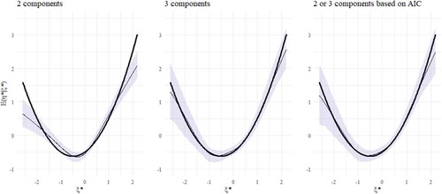
The conditional expected mean $E\left({\text{etaa}}^{\ast }|{\xi }^{\ast }\right)$ is shown as a function of ${\xi }^{\ast }$ in Figure 1 when 2 and 3 components are used (left and middle panels), respectively. The bold line represents the population function in equation (10)(10) ${\text{etaa}}^{\ast }=-0.5+0.5{\text{xia}}^{\ast }+0.5{\text{xia}}^{\ast 2}+\zeta ,$(10) , whereas the thin line represents the average estimated conditional mean function. Ninety-five percent of the estimated functions are within the shaded areas. With two components the functional form is captured to some degree, although the performance is substantially better using three components. Although the average result is acceptable, in some instances, the form of the conditional expected mean is jumping peculiarly when one of the proportions is estimated to be close to zero. In practice, it is difficult to know how many components to use. One possibility is to use the Akaike information criterion (AIC) for selecting the number of components. The AIC is defined as

$\mathrm{A}\mathrm{I}\mathrm{C}=2k-2\mathrm{\ell }\left(\hat{\theta }\right),$

Figure 1. The conditional mean of the true data generating process (thick line) and the average estimated conditional mean (thin line) with empirical 95% intervals (filled blue areas) for 2 components (left), 3 components (middle) and when AIC is used for selecting the number of components (right)

where $k$ is the number of estimated parameters and $\mathrm{\ell }\left(\widehat{\text{thetaa}}\right)$ is the approximated log likelihood at the mode. In the simulations, 3 components are recommended in approximately 84% of the replications. In the right panel of Figure 1, each replication has been estimated using 2 and 3 components and the model with the lowest AIC has been selected. The average estimated conditional mean function (the thin line) captures the population function well.

Discussion and conclusion

In NSEM it is common to consider terms corresponding to interaction and quadratic effects for modeling nonlinearities in the structural model. It is sometimes appropriate to consider more flexible functions with less, or no a priori assumptions about the functional form. Such models are less common in the literature, particularly models which consider ordinal data. In this article, a semiparametric structural model (Bauer, 2005; Pek et al., 2011) is proposed in the presence of ordinal data. The structural model consists of a weighted sum of locally linear functions, which together approximate a globally nonlinear function. A hybrid of a direct maximization approach (Jin et al., 2020) and an expectation-maximization algorithm (Dempster et al., 1977) is suggested and implemented for maximizing the marginal log-likelihood of the observed ordinal data. Two simulation studies are performed. The first shows that the proposed method provides parameter estimates with low relative bias, whereas the second study illustrates how the method accurately captures a nonlinear structural model in terms of the conditional mean of the latent endogenous variable. The accurate parameter estimates and performance in estimating the conditional mean suggest that the AGHQ approximations are of high quality for $q\ge 5$ in models similar to those investigated in this study. Two and three components are used in the second study. Using two components yields a reasonable and stable functional form, whereas three components yield a more accurate functional form on average, with the drawback of occasionally unstable estimates. The number of components might possibly be selected using AIC. Advantages of the proposed method include the capacity of modeling flexible structural models in the presence of ordinal data when the latent exogenous variables are not necessarily normal. In this study, little attention is devoted to the latter point. A suggestion for future studies is to investigate the performance of the proposed method under moderate to severe nonnormality of latent exogenous variables. This is left as a future project.

Correction Statement

This article has been republished with minor changes. These changes do not impact the academic content of the article.

Additional information

Funding

The research reported in this article has been supported by Vetenskapsrådet (Swedish Research Council) under the program “New Statistical Methods for Latent Variable Models, 2017-01175”.

Notes

¹ The subscripts on $X$ and $Y$ should in principle be different, e.g., $j_x$ and $j_y$ but for notational convenience, we use the same ($j$) for $X$ and $Y$.

² A simple structure is not necessary, but in this first study, a simple structure is employed for simplicity.

 

Appendix A

Integral approximation

The integrals in equation (9)(9) $\mathrm{\ell }\left(\theta \right)=\sum _{i=1}^{n}log\sum _{m_i=1}^M\int f\left({\mathit{y}}_i,{\mathit{x}}_i,{\mathrm{{\rm Y}}}_i,m_i\right)d{\mathrm{{\rm Y}}}_i,$(9) are intractable. In this work, such integrals are approximated using the AGHQ approximation. The Gauss-Hermite quadrature approximation of the $K$-dimensional integral $\int exp\left\{g\left(\mathit{t}\right)\right\}d\mathit{t}$ is a weighed sum of function values as

(11) $\sum _{k_1=1}^q\cdots \sum _{k_K=1}^q{w}_{k_1{k}_2\dots k_K}^{\ast }exp\left\{g\left(z_{k_1},\dots ,z_{k_K}\right)\right\},$(11)

where

(12) $w_{k_1{k}_2\dots k_K}^{\ast }=\prod _{j=1}^K{w}_{k_j}exp\left\{z_{k_j}^2\right\},$(12)

where $z_{k_j}$ and $w_{k_j}$ are the Gauss-Hermite quadrature points and weights, respectively. $q$ is the number of quadrature points per dimension. In adaptive Gauss-Hermite quadrature approximation, proposed by Liu and Pierce (1994), the quadrature points are translated and dilated to improve the approximation of unimodel functions $g\left(\mathit{t}\right)$.

 

Appendix B

Maximum Likelihood Estimation

Define

(13) $h_{i,m_i}\left({\mathrm{{\rm Y}}}_i;\theta \right)=logf\left({\mathit{y}}_i,{\mathit{x}}_i,{\mathrm{{\rm Y}}}_i,m_i;\theta \right).$(13)

Then, (5) yields

$h_{i,m_i}\left({\mathrm{{\rm Y}}}_i;\theta \right)=logf\left({\mathit{y}}_i|{\eta }_i\right)+logf\left({\mathit{x}}_i|{\text{xia}}_i\right)+logf\left({\eta }_i|{\xi }_i,m_i\right)+f\left({\text{xia}}_i|m_i\right)+logf\left(m_i\right).$

Equations (3)(3) $g_j^{(x)}\left(P\left(X_j\le u_j|\xi \right)\right)={\alpha }_{x,j}^{(u_j)}-{\beta }_{x,j}^T\xi ,u_j\in \left\{1,\dots ,U_j\right\},j=1,2,\dots ,{\rho }_x,$(3) , (4(4) $g_j^{(y)}\left(P\left(Y_j\le v_j|\eta \right)\right)={\alpha }_{y,j}^{(v_j)}-{\beta }_{y,j}^T\eta ,v_j\in \left\{1,\dots ,V_j\right\},j=1,2,\dots ,{\rho }_y,$(4) ), (6(6) $\xi |m\sim N\left(\xi ;{\text{mua}}^{(m)},{\mathbf{\Phi }}^{(m)}\right)$(6) ), (7(7) $f\left(m\right)={\pi }^{(m)},m=1,2,\dots ,M,$(7) ), (8(8) $\eta |\xi ,m\sim N\left(\eta ;{\tau }^{(m)}+{\mathbf{\Gamma }}^{(m)}\xi ,\mathbf{\Psi }\right).$(8) ) and (13(13) $h_{i,m_i}\left({\mathrm{{\rm Y}}}_i;\theta \right)=logf\left({\mathit{y}}_i,{\mathit{x}}_i,{\mathrm{{\rm Y}}}_i,m_i;\theta \right).$(13) ) give

$h_{i,m_i}\left({\mathrm{{\rm Y}}}_i;\theta \right)=\sum _{j=1}^{{\rho }_x}logP\left(X_{ij}=u_{ij}|{\xi }_i\right)+\sum _{j=1}^{{\rho }_x}P\left(Y_{ij}=v_{ij}|{\eta }_i\right)$

$-\frac{K_{\eta }}{2}log\left(2\pi \right)-\frac{1}{2}log|\mathbf{\Psi }|-\frac{1}{2}{\left({\eta }_i-{\tau }^{(m_i)}-{\text{Gammaa}}^{(m_i)}{\xi }_i\right)}^T{\mathbf{\Psi }}^{-1}\left({\eta }_i-{\tau }^{(m_i)}-{\text{Gammaa}}^{(m_i)}{\xi }_i\right)$

$-\frac{K_{\xi }}{2}log\left(2\pi \right)-\frac{1}{2}log|{\mathbf{\Phi }}^{(m_i)}|-\frac{1}{2}{\left({\mu }^{(m_i)}-{\xi }_i\right)}^T{\left[{\mathbf{\Phi }}^{(m_i)}\right]}^{-1}\left({\text{mua}}^{(m_i)}-{\xi }_i\right)+log{\pi }^{(m_i)}.$

Measurement Model Estimation

Since the sum in (9) does not depend on the parameters in ${\theta }_1$, direct maximization, as proposed by Jin et al. (2020) is implemented for ${\theta }_1$ given the current estimates of ${\theta }_2$. The observed likelihood is

(14) $\mathcal{L}\left(\theta \right)=\prod _{i=1}^n{\mathcal{L}}_i\left(\theta \right)=\prod _{i=1}^n\sum _{m_i=1}^M\int exp\left\{h_{i,m_i}\left({\mathrm{{\rm Y}}}_i;\theta \right)\right\}d{\mathrm{{\rm Y}}}_i.$(14)

where ${\mathcal{L}}_i$ is the observed likelihood of the $i^{th}$ observation. Let the mode ${\widehat{\mathrm{{\rm Y}}}}_{i,m}$ be the solution to

$\frac{\mathrm{\partial }{h}_{i,m_i}}{\mathrm{\partial }{\mathrm{{\rm Y}}}_i}=\mathbf{0},$

and the Hessian be

${\mathit{H}}_{i,m_i}=\frac{{\mathrm{\partial }}^2{h}_{i,m_i}}{\mathrm{\partial }{\mathrm{{\rm Y}}}_i\mathrm{\partial }{\mathrm{{\rm Y}}}_i^T},$

evaluated at the mode. Further, let ${\mathit{L}}_{i,m_i}{\mathit{L}}_{i,m_i}^T={\left(-{\mathit{H}}_{i,m_i}\left({\widehat{\mathrm{{\rm Y}}}}_{i,m_i};\theta \right)\right)}^{-1}$. Applying the AGHQ approximation using equations (11)(11) $\sum _{k_1=1}^q\cdots \sum _{k_K=1}^q{w}_{k_1{k}_2\dots k_K}^{\ast }exp\left\{g\left(z_{k_1},\dots ,z_{k_K}\right)\right\},$(11) and (12(12) $w_{k_1{k}_2\dots k_K}^{\ast }=\prod _{j=1}^K{w}_{k_j}exp\left\{z_{k_j}^2\right\},$(12) ) to the $i^{th}$ factor of equation (14)(14) $\mathcal{L}\left(\theta \right)=\prod _{i=1}^n{\mathcal{L}}_i\left(\theta \right)=\prod _{i=1}^n\sum _{m_i=1}^M\int exp\left\{h_{i,m_i}\left({\mathrm{{\rm Y}}}_i;\theta \right)\right\}d{\mathrm{{\rm Y}}}_i.$(14) , gives

${\mathcal{L}}_i\left(\theta \right)\approx \sum _{m_i=1}^{M}exp\left[\frac{K}{2}log2-\frac{1}{2}log\left|-{\mathit{H}}_{i,m_i}\left({\widehat{\mathrm{{\rm Y}}}}_{i,m_i};\theta \right)\right|\right]\times$

(15) $\sum _{k_1=1}^q\cdots \sum _{k_K=1}^q\left\{w_{k_1,k_2,\dots ,k_K}^{\ast }exp\left[h_i\left({\widetilde{\mathrm{{\rm Y}}}}_{i,m_i}({\mathit{z}}_{k_1},{\mathit{z}}_{k_2},\dots ,z_{k_K});\theta \right)\right]\right\}.$(15)

where ${\widetilde{\mathrm{{\rm Y}}}}_{i,m_i}(k_1,k_2,\dots ,k_K)=\sqrt{2}{\mathit{L}}_{i,m_i}{\mathit{z}}_{k_1,k_2,\dots ,k_K}+{\widehat{\mathrm{{\rm Y}}}}_{i,m_i}$ are the translated and dilated latent variables about the mode. And with ${\mathrm{\ell }}_i\left(\theta \right)=log{\mathcal{L}}_i\left(\theta \right)$ the corresponding observed log-likelihood is

$\mathrm{\ell }\left(\theta \right)=\sum _{i=1}^n{\mathrm{\ell }}_i\left(\theta \right)\approx \sum _{i=1}^{n}log\sum _{m_i=1}^M{e}^{{\mathrm{\ell }}_{i,m}^{(aghq)}\left(\theta ,{\widehat{\mathrm{{\rm Y}}}}_{i,m_i}\right)},$

where ${\mathrm{\ell }}_{i,m}^{(aghq)}\left(\theta ,{\widehat{\mathrm{{\rm Y}}}}_{i,m_i}\right)$ is the log of the $m_i^{th}$ term in equation (15)(15) $\sum _{k_1=1}^q\cdots \sum _{k_K=1}^q\left\{w_{k_1,k_2,\dots ,k_K}^{\ast }exp\left[h_i\left({\widetilde{\mathrm{{\rm Y}}}}_{i,m_i}({\mathit{z}}_{k_1},{\mathit{z}}_{k_2},\dots ,z_{k_K});\theta \right)\right]\right\}.$(15) . ${\theta }_1$ is updated by solving

(16) $\frac{\mathrm{\partial }\mathrm{\ell }}{\mathrm{\partial }{\theta }_1}=\mathbf{0}$(16)

with respect to ${\theta }_1$, using the approximation in equation (15)(15) $\sum _{k_1=1}^q\cdots \sum _{k_K=1}^q\left\{w_{k_1,k_2,\dots ,k_K}^{\ast }exp\left[h_i\left({\widetilde{\mathrm{{\rm Y}}}}_{i,m_i}({\mathit{z}}_{k_1},{\mathit{z}}_{k_2},\dots ,z_{k_K});\theta \right)\right]\right\}.$(15) . Then equation (16)(16) $\frac{\mathrm{\partial }\mathrm{\ell }}{\mathrm{\partial }{\theta }_1}=\mathbf{0}$(16) is

$\frac{\mathrm{\partial }\mathrm{\ell }}{\mathrm{\partial }{\theta }_1}\approx \sum _{i=1}^n\frac{{\sum }_{m_i=1}^M\frac{\mathrm{\partial }{\mathrm{\ell }}_{i,m_i}^{(aghq)}(\theta ,{\widehat{\mathrm{{\rm Y}}}}_{i,m_i})}{\mathrm{\partial }{\theta }_1}exp\left\{{\mathrm{\ell }}_{i,m_i}^{(aghq)}({\widehat{\mathrm{{\rm Y}}}}_{i,m_i};\theta )\right\}}{{\sum }_{m_i=1}^{M}exp\left\{{\mathrm{\ell }}_{i,m_i}^{(aghq)}({\widehat{\mathrm{{\rm Y}}}}_{i,m_i};\theta )\right\}}.$

Acknowledging that the mode ${\widehat{\mathrm{{\rm Y}}}}_{i,m_i}$ depends on $\theta$, the gradient of ${\mathrm{\ell }}_{i,m}\left(\theta ,{\widehat{\mathrm{{\rm Y}}}}_{i,m}(\theta )\right)$ is

(17) $\frac{\mathrm{\partial }{\mathrm{\ell }}_{i,m_i}\left(\theta ,{\widehat{\mathrm{{\rm Y}}}}_{i,m_i}(\theta )\right)}{\mathrm{\partial }{\theta }_1}=\frac{\mathrm{\partial }{\mathrm{\ell }}_{i,m_i}(\theta )}{\mathrm{\partial }{\theta }_1}{|}_{\mathrm{{\rm Y}}={\widehat{\mathrm{{\rm Y}}}}_{i,m_i}}+{\left(\frac{\mathrm{\partial }{\widehat{\mathrm{{\rm Y}}}}_{i,m_i}(\theta )}{\mathrm{\partial }{\theta }^T}\right)}^T\frac{\mathrm{\partial }{\mathrm{\ell }}_{i,m_i}(\mathrm{{\rm Y}})}{\mathrm{\partial }\mathrm{{\rm Y}}}{|}_{\mathrm{{\rm Y}}={\widehat{\mathrm{{\rm Y}}}}_{i,m_i}},$(17)

where $\mathrm{\partial }{\mathrm{\ell }}_{i,m_i}(\theta )/\mathrm{\partial }{\theta }_1$ is the derivative of ${\mathrm{\ell }}_{i,m_i}$ with respect to ${\theta }_1$, treating ${\widehat{\mathrm{{\rm Y}}}}_{i,m_i}$ as constant, whereas $\mathrm{\partial }{\mathrm{\ell }}_{i,m_i}(\mathrm{{\rm Y}})/\mathrm{\partial }\mathrm{{\rm Y}}$ is the derivative of ${\mathrm{\ell }}_{i,m_i}$ with respect to the latent variables, treating $\theta$ as fixed. The first factor in the second term of (17) is, by the implicit function theorem

$\frac{\partial {\widehat{{\rm Y}}}_{i,m}(\theta )}{\partial {\theta }_1^T}=-{\left(\frac{{\partial }^2{h}_i\left({\rm Y};\theta \right)}{\partial {\rm Y}\partial {{\rm Y}}^T}{|}_{{{\rm Y}}_{i,m}={\widehat{{\rm Y}}}_{i,m}}\right)}^{-1}\frac{{\partial }^2{h}_{i,m}\left({\rm Y};\theta \right)}{\partial {\rm Y}\partial {\theta }_1^T}{|}_{{{\rm Y}}_{i,m}={\widehat{{\rm Y}}}_{i,m}}.$

In order to find the solution to equation (16)(16) $\frac{\mathrm{\partial }\mathrm{\ell }}{\mathrm{\partial }{\theta }_1}=\mathbf{0}$(16) the BFGS approximation to the Newton–Raphson method is implemented. The inverse of ${\mathit{H}}_{i,m_i}$ is approximated and updated by low-rank approximation at each iteration. The updated parameter vector ${\theta }_1$ is obtained by updating ${\theta }_1$ with the BFGS algorithm a number of times.

Structural Model Estimation

If the quasi-Newton-Raphson method proposed in the previous section would be used, the sum in equation (14)(14) $\mathcal{L}\left(\theta \right)=\prod _{i=1}^n{\mathcal{L}}_i\left(\theta \right)=\prod _{i=1}^n\sum _{m_i=1}^M\int exp\left\{h_{i,m_i}\left({\mathrm{{\rm Y}}}_i;\theta \right)\right\}d{\mathrm{{\rm Y}}}_i.$(14) introduces instability for parameters, which depend on $m_i$. All elements in ${\theta }_2$ depend on $m_i$ except for $\mathbf{\Psi }$. $\mathbf{\Psi }$ is the same for all $m_i$ in this setting only for simplicity. The reason for keeping $\mathbf{\Psi }$ in ${\theta }_2$ is for convenience at later stages in more general settings. The EM algorithm of Dempster et al. (1977) is implemented for updating ${\theta }_2$ given the current estimates of ${\theta }_1$, as follows:

Treating ${\mathrm{{\rm Y}}}_i$ and $m_i$ as random variables, let the conditional distribution of ${\mathrm{{\rm Y}}}_i$ and $m_i$ be

(18) $f_i\left({\mathrm{{\rm Y}}}_i,m_i|{\mathit{y}}_i,{\mathit{x}}_i;{\theta }_1,{\theta }_2^{(old)}\right)=\frac{f_i\left({\mathit{y}}_i,{\mathit{x}}_i,{\mathrm{{\rm Y}}}_i,m_i;{\theta }_1,{\theta }_2^{(old)}\right)}{{\sum }_{m=1}^M\int \int f_i\left({\mathit{y}}_i,{\mathit{x}}_i,{\mathrm{{\rm Y}}}_i,m_i;{\theta }_1,{\theta }_2^{(old)}\right)d{\mathrm{{\rm Y}}}_i}$(18)

at the current iteration given the parameter values obtained in the previous iteration, ${\theta }_2^{(old)}$. The update of ${\theta }_2$ is the vector that maximizes the expected value of the complete log-likelihood given the conditional distribution in equation (18)(18) $f_i\left({\mathrm{{\rm Y}}}_i,m_i|{\mathit{y}}_i,{\mathit{x}}_i;{\theta }_1,{\theta }_2^{(old)}\right)=\frac{f_i\left({\mathit{y}}_i,{\mathit{x}}_i,{\mathrm{{\rm Y}}}_i,m_i;{\theta }_1,{\theta }_2^{(old)}\right)}{{\sum }_{m=1}^M\int \int f_i\left({\mathit{y}}_i,{\mathit{x}}_i,{\mathrm{{\rm Y}}}_i,m_i;{\theta }_1,{\theta }_2^{(old)}\right)d{\mathrm{{\rm Y}}}_i}$(18) . Throughout this section, ${\theta }_1$ is fixed to the current estimate. Hence, for simplicity, ${\theta }_1$ is dropped. Then, the objective function is

(19) $Q\left({\theta }_2,{\theta }_2^{(old)}\right)=\sum _{i=1}^n{Q}_i\left({\theta }_2,{\theta }_2^{(old)}\right)$(19)

$=\sum _{i=1}^n\frac{{\sum }_{m_i=1}^M\int h_{i,m_i}\left({\mathrm{{\rm Y}}}_i;{\theta }_2\right)f_i\left({\mathit{y}}_i,{\mathit{x}}_i,{\mathrm{{\rm Y}}}_i,m_i;{\theta }_2^{(old)}\right)d{\mathrm{{\rm Y}}}_i}{{\sum }_{m_i=1}^M\int f_i\left({\mathit{y}}_i,{\mathit{x}}_i,{\mathrm{{\rm Y}}}_i,m_i;{\theta }_2^{(old)}\right)d{\mathrm{{\rm Y}}}_i}.$

The maximum of (19) is attained at ${\theta }_2^{(upd)}$ and can be expressed in terms of the following integrals:

$\int f_i\left({\mathit{y}}_i,{\mathit{x}}_i,{\mathrm{{\rm Y}}}_i,m;{\theta }_2^{(old)}\right)d{\mathrm{{\rm Y}}}_i\equiv {\rho }_{i,m}$

$\int {\xi }_i{f}_i\left({\mathit{y}}_i,{\mathit{x}}_i,{\mathrm{{\rm Y}}}_i,m;{\theta }_2^{(old)}\right)d{\mathrm{{\rm Y}}}_i\equiv {\rho }_{\xi ;i,m}$

$\int {\eta }_i{f}_i\left({\mathit{y}}_i,{\mathit{x}}_i,{\mathrm{{\rm Y}}}_i,m;{\theta }_2^{(old)}\right)d{\text{Upsilona}}_{\mathbf{i}}\equiv {\rho }_{\eta ,:i,m}$

$\int {\text{xia}}_i{\text{xia}}_i^T{f}_i\left({\mathit{y}}_i,{\mathit{x}}_i,{\mathrm{{\rm Y}}}_i,m;{\theta }_2^{(old)}\right)d{\mathrm{{\rm Y}}}_i\equiv {\mathbf{\Delta }}_{\xi \xi ;i,m}$

$\int {\eta }_i{\eta }_i^T{f}_i\left({\mathit{y}}_i,{\mathit{x}}_i,{\mathrm{{\rm Y}}}_i,m;{\theta }_2^{(old)}\right)d{\text{Upsilona}}_i\equiv {\mathbf{\Delta }}_{\text{etaa}\text{etaa};i,m}$

(20) $\int {\text{xia}}_i{\eta }_i^T{f}_i\left({\mathit{y}}_i,{\mathit{x}}_i,{\mathrm{{\rm Y}}}_i,m;{\theta }_2^{(old)}\right)d{\text{Upsilona}}_i\equiv {\mathbf{\Delta }}_{\xi \text{etaa};i,m},$(20)

and the current estimate of the effective number of observations per component

${\hat{n}}^{(m)}=\sum _{i=1}^n\frac{{\rho }_{i,m}}{{\sum }_{l=1}^M{\rho }_{i,l}}.$

Then the updated parameter vector ${\theta }_2^{(upd)}$ is composed of

${\tau }_{(upd)}^{(m)}=\frac{1}{{\hat{n}}^{(m)}}\sum _{i=1}^n\frac{{\rho }_{\text{etaa},:i,m}-{\mathbf{\Gamma }}_{(old)}^{(m)}{\rho }_{\xi ;i,m}}{{\sum }_{l=1}^M{\rho }_{i,l}}$

${\mathbf{\Gamma }}_{(upd)}^{(m)}=\left[\sum _{i=1}^n\frac{{\mathbf{\Delta }}_{\xi \text{etaa};i,m}^T-{\text{tauu}}_{(old)}^{(m)}{\text{rhoa}}_{\xi ;i,m}^T}{{\sum }_{l=1}^M{\rho }_{i,l}}\right]{\left[\sum _{i=1}^n\frac{{\mathbf{\Delta }}_{\xi \xi ;i,m}}{{\sum }_{l=1}^M{\rho }_{i,l}}\right]}^{-1}$

${\mathbf{\Phi }}_{(upd)}^{(m)}={\text{mua}}_{(old)}^{(m)}{\left({\text{mua}}_{(old)}^{(m)}\right)}^T+\frac{1}{{\hat{n}}^{(m)}}\left[\sum _{i=1}^n\frac{{\mathbf{\Delta }}_{\xi \xi ;i,m}-{\text{mua}}_{(old)}^{(m)}{\rho }_{\xi ;i,m}^T-{\rho }_{\xi ;i,m}{\left({\text{mua}}_{(old)}^{(m)}\right)}^T}{{\sum }_{l=1}^M{\rho }_{i,l}}\right]$

${\text{mua}}_{(upd)}^{(m)}=\frac{1}{{\hat{n}}^{(m)}}\sum _{i=1}^n\frac{{\rho }_{\xi ;i,m}}{{\sum }_{l=1}^M{\rho }_{i,l}}$

${\pi }_{(upd)}^{(m)}=\frac{{\hat{n}}^{(m)}}{n},$

for $m=1,\dots ,M$, and

${\mathbf{\Psi }}_{(upd)}=\frac{1}{n}\sum _{i=1}^n\frac{\text{Omegaa}}{{\sum }_{l=1}^M{\rho }_{i,l}},$

where

$\text{Omegaa}=\sum _{l=1}^M{\mathbf{\Delta }}_{\text{etaa}\text{etaa};i,l}-{\rho }_{\text{etaa},:i,l}{\left[{\tau }_{(old)}^{(l)}\right]}^T-{\tau }_{(old)}^{(l)}{\rho }_{\text{etaa},:i,l}^T-{\mathbf{\Delta }}_{\xi \text{etaa};i,l}^T{\left[{\mathbf{\Gamma }}_{(old)}^{(l)}\right]}^T-{\mathbf{\Gamma }}_{(old)}^{(l)}{\mathbf{\Delta }}_{\xi \text{etaa};i,l}$

$+{\tau }_{(old)}^{(l)}{\left[{\tau }_{(old)}^{(l)}\right]}^T{\rho }_{i,m}+{\tau }_{(old)}^{(l)}{\rho }_{\xi ;i,l}^T{\left[{\mathbf{\Gamma }}_{(old)}^{(l)}\right]}^T+{\mathbf{\Gamma }}_{(old)}^{(l)}{\rho }_{\xi ;i,l}{\left[{\tau }_{(old)}^{(l)}\right]}^T+{\mathbf{\Gamma }}_{(old)}^{(l)}{\mathbf{\Delta }}_{\xi \xi ;i,l}{\left[{\mathbf{\Gamma }}_{(old)}^{(l)}\right]}^T.$

The integrals in (36) are intractable. For ${\rho }_{i,m}$ the AGHQ approximation is applied as in the previous section. For the other integrals, the same weights and quadrature points are used. Integrals should still be asymptotically well approximated since the original integrand is multiplied by a polynomial of degree at most 2, as argued by Naylor and Smith (1982). Once the updated estimates are obtained the previous estimates ${\theta }_2^{(old)}$ are replaced by the updated ${\theta }_2^{(upd)}$ and the procedure is repeated a number of times.

References

- Agustin, C., & Singh, J. (2005). Curvilinear effects of consumer loyalty determinants in relational exchanges. Journal of Marketing Research, 42, 96–108. https://doi.org/10.1509/jmkr.42.1.96.56961
- Ajzen, I. (1991). The theory of planned behavior. Organizational Behavior and Human Decision Processes, 50, 179–211. https://doi.org/10.1016/0749-5978(91)90020-T
- Ajzen, I., & Madden, T. J. (1986). Prediction of goal-directed behavior: Attitudes, intentions, and perceived behavioral control. Journal of Experimental Social Psychology, 22, 453–474. https://doi.org/10.1016/0022-1031(86)90045-4
- Arminger, G., & Muthén, B. O. (1998). A Bayesian approach to nonlinear latent variable models using the Gibbs sampler and the Metropolis-Hastings algorithm. Psychometrika, 63, 271–300. https://doi.org/10.1007/BF02294856
- Bauer, D. J. (2005). A semiparametric approach to modeling nonlinear relations among latent variables. Structural Equation Modeling: A Multidisciplinary Journal, 12, 513–535. https://doi.org/10.1207/s15328007sem1204_1
- Bollen, K. A. (1995). Structural equation models that are nonlinear in latent variables: A least-squares estimator. In Sociological methodology (pp. 223–251). Washington, DC: American Sociological Association.
- Bollen, K. A. (1996). An alternative two stage least squares (2SLS) estimator for latent variable equations. Psychometrika, 61, 109–121. https://doi.org/10.1007/BF02296961
- R Core Team (2018). R: A language and environment for statistical computing. Vienna, AU: R Foundation for Statistical Computing.
- Dempster, A. P., Laird, N. M., & Rubin, D. B. (1977). Maximum likelihood from incomplete data via the em algorithm. Journal of the Royal Statistical Society. Series B (Methodological), 39, 1–38. https://www.jstor.org/stable/2984875
- Finch, W. H. (2015). Modeling nonlinear structural equation models: A comparison of the two-stage generalized additive models and the finite mixture structural equation model. Structural Equation Modeling: A Multidisciplinary Journal, 22, 60–75. https://doi.org/10.1080/10705511.2014.935749
- Finney, S. J., & DiStefano, C. (2006). Structural equation modeling: A second course. Information Age Publishing.
- Flora, D. B., & Curran, P. J. (2004). An empirical evaluation of alternative methods of estimation for confirmatory factor analysis with ordinal data. Psychological Methods, 9, 446–491. https://doi.org/10.1037/1082-989X.9.4.466
- Guo, R., Zhu, H., Chow, S.-M., & Ibrahim, J. G. (2012). Bayesian lasso for semiparametric structural equation models. Biometrics, 68, 567–577. https://doi.org/10.1111/j.1541-0420.2012.01751.x
- Harring, J. R., Weiss, B. A., & Hsu, J.-C. (2012). A comparison of methods for estimating quadratic effects in nonlinear structural equation models. Psychological Methods, 17, 193. https://doi.org/10.1037/a0027539
- Jaccard, J., & Wan, C. K. (1995). Measurement error in the analysis of interaction effects between continuous predictors using multiple regression: Multiple indicator and structural equation approaches. Psychological Bulletin, 117(2), 348–357. https://doi.org/10.1037/0033-2909.117.2.348
- Jin, S., & Andersson, B. (2020). A note on the accuracy of adaptive Gauss–Hermite quadrature. Biometrika, 107, 737–744. https://doi.org/10.1093/biomet/asz080
- Jin, S., Vegelius, J., & Yang-Wallentin, F. (2020). A marginal maximum likelihood approach for extended quadratic structural equation modeling with ordinal data. Advance Online Publication in Structural Equation Modeling: A Multidisciplinary Journal, 1–10. https://doi.org/10.1080/10705511.2020.1712552
- Jöreskog, K. G., & Sörbom, D. (1993). New features in lisrel 8. Scientific Software.
- Jöreskog, K. G., & Sörbom, D. (1996). LISREL 8: User’s reference guide. Scientific Software International.
- Jöreskog, K. G., & Yang, F. (1996). Non-linear structural equation models: The kenny-judd model with interaction effects. In G. A. Marcoulides & R. E. Schumacker (Eds.), Advanced structural equation modeling: Issues and techniques (pp. 57–88). Lawrence Erlbaum Associates.
- Kelava, A., & Brandt, H. (2009). Estimation of nonlinear latent structural equation models using the extended unconstrained approach. Review of Psychology, 16, 123–132. https://hrcak.srce.hr/70644
- Kelava, A., Nagengast, B., & Brandt, H. (2014). A nonlinear structural equation mixture modeling approach for nonnormally distributed latent predictor variables. Structural Equation Modeling: A Multidisciplinary Journal, 21, 468–481. https://doi.org/10.1080/10705511.2014.915379
- Kenny, D. A., & Judd, C. M. (1984). Estimating the nonlinear and interactive effects of latent variables. Psychological Bulletin, 96, 201–210. https://doi.org/10.1037/0033-2909.96.1.201
- Klein, A., & Moosbrugger, H. (2000). Maximum likelihood estimation of latent interaction effects with the LMS method. Psychometrika, 65, 457–474. https://doi.org/10.1007/BF02296338
- Klein, A., & Muthén, B. (2007). Quasi-maximum likelihood estimation of structural equation models with multiple interaction and quadratic effects. Multivariate Behavioral Research, 42, 647–673. https://doi.org/10.1080/00273170701710205
- Lee, S.-Y., & Song, X.-Y. (2003). Model comparison of nonlinear structural equation models with fixed covariates. Psychometrika, 68, 27–47. https://doi.org/10.1007/BF02296651
- Lee, S.-Y., & Zhu, H.-T. (2000). Statistical analysis of nonlinear structural equation models with continuous and polytomous data. British Journal of Mathematical and Statistical Psychology, 53, 209–232. https://doi.org/10.1348/000711000159303
- Liu, Q., & Pierce, D. A. (1994). A note on Gauss-Hermite quadrature. Biometrika, 81, 624–629. https://doi.org/10.2307/2337136
- Muthén, B. (2001). Second-generation structural equation modeling with a combination of categorical and continuous latent variables: New opportunities for latent class/latent growth modeling. In L. M. Collins, & A. Sayer (Eds.), New methods for the analysis of change (pp. 291–322). Washington, DC: APA.
- Muthén, L., & Muthén, B. (2020). Mplus. The comprehensive modelling program for applied researchers: user’s guide, 5. Los Angeles, CA: Muthén & Muthén.
- Naylor, J. C., & Smith, A. F. (1982). Applications of a method for the efficient computation of posterior distributions. Journal of the Royal Statistical Society. Series C, Applied Statistics, 31, 214–225. https://doi.org/10.2307/2347995
- Pek, J., Losardo, D., & Bauer, D. J. (2011). Confidence intervals for a semiparametric approach to modeling nonlinear relations among latent variables. Structural Equation Modeling: A Multidisciplinary Journal, 18, 537–553. https://doi.org/10.1080/10705511.2011.607072
- Rhemtulla, M., Brosseau-Liard, P. E., & Savalei, V. (2012). When can categorical variables be treated as continuous? A comparison of robust continuous and categorical sem estimation methods under suboptimal condition. Psychological Methods, 17, 354–373. https://doi.org/10.1037/a0029315
- Rizopoulos, D., & Moustaki, I. (2008). Generalized latent variable models with non-linear effects. British Journal of Mathematical and Statistical Psychology, 61, 415–438. https://doi.org/10.1348/000711007X213963
- Song, X.-Y., Lu, Z., & Feng, X. (2014). Latent variable models with nonparametric interaction effects of latent variables. Statistics in Medicine, 33, 1723–1737. https://doi.org/10.1002/sim.6065
- Song, X.-Y., & Lu, Z.-H. (2010). Semiparametric latent variable models with bayesian p-splines. Journal of Computational and Graphical Statistics, 19, 590–608. https://doi.org/10.1198/jcgs.2010.09094
- Song, X.-Y., Lu, Z.-H., Cai, J.-H., & Ip, E. H.-S. (2013). A bayesian modeling approach for generalized semiparametric structural equation models. Psychometrika, 78, 624–647. https://doi.org/10.1007/s11336-013-9323-7
- Wall, M. M. (2009). Maximum likelihood and bayesian estimation for nonlinear structural equation models. In R. E. Millsap & A. Maydeu-Olivares (Eds.), The SAGE handbook of quantitative methods in psychology (pp. 540–567). London: Sage Publications Ltd.
- Wall, M. M., & Amemiya, Y. (2001). Generalized appended product indicator procedure for nonlinear structural equation analysis. Journal of Educational and Behavioral Statistics, 26, 1–29. https://doi.org/10.3102/10769986026001001
- Zhu, H.-T., & Lee, S.-Y. (1999). Statistical analysis of nonlinear factor analysis models. British Journal of Mathematical and Statistical Psychology, 52, 225–242. https://doi.org/10.1348/000711099159080