
 ?Mathematical formulae have been encoded as MathML and are displayed in this HTML version using MathJax in order to improve their display. Uncheck the box to turn MathJax off. This feature requires Javascript. Click on a formula to zoom.
ABSTRACT
Bayesian estimation of multilevel structural equation models (MLSEMs) offers advantages in terms of sample size requirements and computational feasibility, but does require careful specification of the prior distribution especially for the random effects variance parameters. The traditional “non-informative” conjugate choice of an inverse-Gamma prior with small hyperparameters has been shown time and again to be problematic. In this paper, we investigate alternative, more robust prior distributions for the doubly latent categorical multilevel model. In contrast to multilevel models without latent variables, MLSEMs have multiple random effects variance parameters both for the multilevel structure and for the latent variable structure. It is therefore even more important to construct reasonable priors for these parameters. We find that, although the robust priors outperform the traditional inverse-Gamma prior, their hyperparameters do require careful consideration.
KEYWORDS:
Introduction
Multilevel structural equation modeling (MLSEM) has become increasingly popular to test complex theories in samples that are hierarchically structured (Muthén, Citation1994). While SEM allows researchers to control for measurement error due to the fact that only a finite number of items are sampled, multilevel analysis takes into account sampling error due to the fact that only a finite number of individuals is sampled. Combined, MLSEM offers a powerful tool that is being used throughout educational, psychological, and sociological research.
Traditionally, maximum likelihood (ML) algorithms have been used to estimate MLSEMs. However, in the case of categorical indicators, such algorithms require multidimensional numerical integration, which quickly becomes computationally infeasible (Asparouhov & Muthen, Citation2007). Weighted least squares (WLS) algorithms avoid the high dimensional integration, but are restricted to random intercept models (Asparouhov & Muthén, Citation2012). Additionally, both ML and WLS rely on the frequentist asymptotical framework and thus require a substantial number of groups to obtain admissible and accurate parameter estimates (Hox & Maas, Citation2001). For example, Meuleman and Billiet (Citation2009) concluded that for relatively simple MLSEMs, at least 60 groups are needed to detect large structural effects at the between level.
Due to these problems with frequentist estimation methods, Bayesian estimation of MLSEMs has become increasingly popular. In a Bayesian analysis, a prior distribution is specified for each of the parameters in the model. Combined with the likelihood of the data this results in a posterior distribution, which is generally obtained through Markov Chain Monte Carlo (MCMC) sampling. The Bayesian approach offers several advantages compared to the frequentist framework. First, MCMC sampling does not require multidimensional numerical integration enabling complex models with categorical indicators to be estimated (see, e.g., Asparouhov & Muthén, Citation2012). Second, estimates of the transformed parameters, such as indirect structural effects, can be easily obtained by transforming the MCMC samples and credible intervals are obtained automatically (Yuan & MacKinnon, Citation2009). Credible intervals are the Bayesian alternative of confidence intervals, but unlike confidence intervals do not rely on normality assumptions or asymptotical theory. Third, through the prior distribution, the problem of variances that are estimated to be negative (i.e., Heywood cases) can be solved; so long as the prior on the variance has zero mass at negative values, the estimate can never become negative. Moreover, prior information about parameters in the model can be included in the prior distribution. This information might be based on previous investigations or expert knowledge. Finally, it has been shown that Bayesian MLSEM can provide accurate estimates with a smaller number of groups compared to frequentist estimation (Hox et al., Citation2012; Zitzmann et al., Citation2016).
A main focus of the Bayesian literature on multilevel models is the specification of the prior for the random effects variance parameter. The random effects variance parameter decides how much pooling across observations takes place. A random effects variance parameter equal to zero implies complete pooling of observations, that is, that there are no random effects and thus that we fit the same regression line for all higher level units. As the value for the random effects variance increases, the amount of pooling decreases until there is no pooling at all, which means that each higher level unit has its own regression line, a solution that will generally overfit the data. The prior for the random effects variance parameter determines where the model lies on this continuum from complete pooling to no pooling. Historically, inverse-Gamma priors were popular choices for variance parameters, including those at the between level, since they are conjugate and thus result in a posterior that is an inverse-Gamma distribution as well. Specifically, an inverse-Gamma (,
) prior with small
has often been used as a default uninformative prior distribution. However, it is now well-known in the literature that for random effects variances, this specification is actually very informative and highly sensitive to the exact choice of the hyperparameters (see, e.g., Gelman, Citation2006; Klein & Kneib, Citation2016; Lunn et al., Citation2009). Moreover, as we will show later, the inverse-Gamma prior does not have support for random effects variances equal to zero and will therefore always favor more complex solutions with less pooling. A second often used class of default priors for variance parameters is the class of uniform improper priors. This is in line with the “objective” Bayesian approach (Berger, Citation2006) since these priors will, in simple models, result in the same estimates as classical ML estimation. Various improper uniform prior options exist. The most straightforward approach is to specify a uniform prior directly on the variance, that is,
. A second option, advocated by Berger (Citation2006), Berger and Strawderman (Citation1996), and Gelman (Citation2006), is to specify a uniform prior on the standard deviation, that is,
. Finally, a uniform prior can be specified on the logarithm of the variance, that is,
. The main issue with specifying improper priors for random effects variances is that the resulting posterior might be improper as well in cases where there is a limited amount of information in the data on the higher level (Berger, Citation2006; Gelman, Citation2006). This has been shown empirically in an SEM where improper priors resulted in lower convergence rates (Van Erp et al., Citation2018). Note that the inverse-Gamma (
,
) prior approximates the improper prior
as
goes to zero. As a result, the inverse-Gamma prior can also lead to an unstable MCMC sampler.
Recently, several weakly informative prior distributions have been proposed as alternative priors for random effects variances. Compared to the uniform improper priors, weakly informative priors perform some shrinkage of the random effects variance parameter toward zero, that is, the complete pooling situation, to avoid overfitting. For example, Gelman (Citation2006) and Polson and Scott (Citation2012) propose to use the half-Cauchy prior, which is proper and thus avoids the issue of uniform improper priors. Additionally, the half-Cauchy prior has heavy tails and is therefore considered robust to misspecification of the scale. Simpson et al. (Citation2017) discuss a general approach to construct so-called “scale dependent” priors, which can be straightforwardly applied to random effects variances. Although some studies exist that compare some of these priors in general multilevel models (see, e.g., Klein & Kneib, Citation2016), they have yet to be investigated in the context of MLSEM. Studies investigating prior choice in MLSEM generally focus on conjugate prior distributions that vary in the degree of informativeness (Depaoli & Clifton, Citation2015; Helm, Citation2018; Zitzmann et al., Citation2016). These studies show that informative priors, when correctly specified, perform best. However, in reality, we do not know the true population value and therefore require prior distributions that are robust against possible prior misspecification. Moreover, MLSEMs have multiple random effects variance parameters, both for the multilevel structure and for the latent variable structure. It is therefore even more important to construct reasonable and robust priors for these parameters.
The goal of this study is to compare robust prior distributions for random effects variances in MLSEM. We will compare default specifications of the robust priors as well as informative (in)accurate specifications. The outline of this paper is as follows: in Section 2 we describe the categorical MLSEM used throughout this paper along with the motivating application from education. The robust prior distributions are presented and compared in Section 3, and Section 4 presents two simulation studies to investigate the performance of the priors, followed by a discussion in Section 5.
Bayesian doubly latent categorical multilevel model
Model
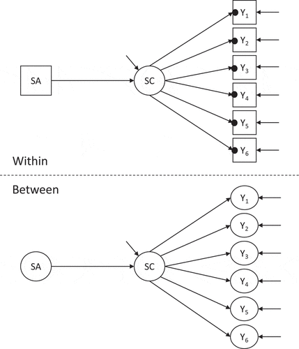
The MLSEM used in this investigation is based on the doubly latent multilevel model (DLMM) proposed in Marsh et al. (Citation2009) to estimate contextual effects. A well-known application of the DLMM is to estimate the “Big-Fish-Little-Pond-Effect” (BFLPE) that predicts that at the individual (or within) level, student achievement has a positive effect on academic self-concept, whereas at the between level, school-average achievement has a negative effect on academic self-concept. The term “doubly latent” arises from the fact that the model takes into account both measurement and sampling error. Measurement error, which is a consequence of the fact that only a finite number of items are sampled, is controlled for by specifying a measurement model for each of the factors. Sampling error, on the other hand, is the result of sampling only a finite number of individuals and is taken into account by including random effects in the model. The model used is depicted in . We use a similar representation as in Marsh et al. (Citation2009).Manifest variables are denoted by squares, while latent variables are denoted by circles. Black dots indicate a random intercept at the between level for that variable.
Figure 1. Graphic representation of the doubly latent multilevel model (DLMM) used throughout this paper. SA stands for student achievement and SC stands for academic self-concept in the context of the “Big-Fish-Little-Pond-Effect” (BFLPE)
We assume that academic self-concept is measured by six binary indicators for individual i in group j measured on item k.Footnote1 We assume an underlying continuous latent response variable
that is linked to the binary observed responses
as follows:
The measurement model can then be defined for the continuous latent responses at the within level:
where denotes the intercept for item
in group
,
is the loading for item
at the within level,
is the factor score for individual
in group
, and
is the residual at the within level for individual i in group j measured on item k. Throughout this paper, we assume a logistic distribution for the residuals at the within level, that is,
and we fix the variance to that of the standard logistic distribution, that is,
for identification.Footnote2
We focus on the random intercept model such that the measurement model at the between level is defined as:
where reflects the overall intercept for item
and is fixed to 0 for identification,
is the loading for item
at the between level,
is the factor score at the between level for group
, and
denotes the residual at the between level for item
in group
, which we assume to be normally distributed, that is,
.
The factor scores on self-concept are predicted by the academic achievement scores leading to the following structural model:
Here, represents the effect of achievement on self-concept at the within level, whereas
represents the effect of achievement on self-concept at the between level. To identify the latent variables, we restrict the mean, that is,
in EquationEquation (5)
(5)
(5) and one loading at each level,Footnote3 that is,
. As recommended by Asparouhov and Muthén (Citation2019), we use latent mean centering which estimates the group mean achievement in each group
, that is,
to take into account measurement error. The parameter of interest is the contextual effect, which equals
.
An important quantity in multilevel models is the variance partition coefficient (VPC; Goldstein et al., Citation2002), which is a measure of the correlation between students in the same school. In multilevel SEM, the VPC for item
is defined as (see EquationEquation (8)
(8)
(8) in Muthen, Citation1991):
Prior distributions
In a Bayesian analysis, prior distributions need to be specified for each parameter in the model, that is, . The focus of this paper is on priors for the random effects variances
and the next section discusses the priors we consider for these parameters in detail. For the other parameters in the model, we use the following independent, uninformative or weakly informative prior distributions throughout this paper:
,
,
. Note that other choices are possible and it is always important to investigate the sensitivity of the results to the specification of the prior distribution (Van Erp et al., Citation2018).
Robust prior distributions for random effects variances
The problems with the traditional inverse-Gamma family and the improper uniform priors for random effects variances have inspired many researchers to investigate alternative, more robust prior distributions. Here, we focus on three such alternative classes of priors: 1) Student’s priors; 2) F priors; and 3) Scale dependent priors. Note that some priors are specified on the variances while others are specified on the standard deviations. Throughout this section, we will use
to denote standard deviations and
to denote variance parameters.
Student’s  family
A widespread proposal for the prior on random effects is to specify a proper, weakly informative half-t distribution on the standard deviation (see, e.g., Gelman, Citation2006; Polson & Scott, Citation2012). The probability density function of the half-t distribution is given by:
where denotes the scale and
the degrees of freedom. Different choices for the scale parameter
are discussed in Subsection “Specification of the hyperparameters”. For the degrees of freedom
, smaller values result in heavier tails. For
, we obtain the half-normal distribution, which has been proposed, among others, by Frühwirth-Schnatter and Wagner (Citation2010). Roos and Held (Citation2011) have shown that the half-normal prior indeed results in estimates of the random effects variances that are less sensitive to the chosen hyperparameters compared to the inverse-Gamma prior. Nevertheless, the half-normal distribution still has very light tails and will therefore be less robust to variance parameters that are larger than expected. Therefore, a more robust proposal in the literature is to specify the degrees of freedom to be smaller. Gelman (Citation2006) notes the special case of the half-Cauchy prior with
as a reasonable default option. The half-Cauchy prior has been further investigated by Polson and Scott (Citation2012), who have shown that it has excellent frequentist risk properties. There are some reports, however, that the heavy tails of the half-Cauchy prior can lead to numerical difficulties in MCMC sampling (Ghosh et al., Citation2018; Piironen & Vehtari, Citation2015). This issue generally arises in situations where there is not enough information in the data such that the parameter is weakly or non-identified. The heavy tails of the (half-)Cauchy prior do not perform enough shrinkage in such cases to identify the parameter.
F family
A popular family of distributions for variance parameters in the Bayesian literature is the family of F priors, also known as scaled Beta2 or generalized beta prime priors (Fúquene et al., Citation2014; Mulder & Pericchi, Citation2018; Pérez et al., Citation2017; Polson & Scott, Citation2012). The probability density function of the F prior is given by (Mulder & Pericchi, Citation2018):Footnote4
where denotes a scale parameter, the degrees of freedom
determines the behavior around zero, and the degrees of freedom
influences the tail behavior in a similar manner as the degrees of freedom for Student’s t distribution. Specifically,
results in similar tails as a Cauchy distribution. With regard to the behavior at zero,
results in a density that is zero at the origin, for
the density is bounded at the origin, and for
the density goes to infinity at the origin.
Interestingly, if , then the prior on the standard deviation
corresponds to a half-Student’s
distribution with degrees of freedom equal to
and scale
. Thus, the F family can be seen as a generalization of the Student’s
family. Moreover, if
, then the prior on the precision
will also be an F distribution, with a scale of
(i.e., the reciprocality property).
To implement the F prior, the following Gamma mixture of inverse-Gamma parametrization can be used:
which results in the F prior when integrating out .
Scale dependent family
Simpson et al. (Citation2017) have proposed the use of penalized complexity priors as general default priors. The basic idea of these priors is that deviations from a simpler base model are penalized thereby avoiding a model that overfits. This characteristic is especially useful in the context of random effects variance parameters which are generally weakly identified due to the small amount of information available at the higher level. Simpson et al. (Citation2017) derive the penalized complexity prior for the precision of a random effect as follows: first, define the base model. For example, for the random effects component in (3), the base model, which is the simplest model in its class, would correspond to
or the absence of random effects. Next, the distance of the flexible extension of the base model, that is,
to the base model is computed based on the Kullback-Leibler divergence (KLD). Simpson et al. (Citation2017) define the distance between the two models with densities
and
as:
. Then, a prior is specified for the distance
such that deviations from the base model are penalized. By assuming a constant rate of penalization, Simpson et al. (Citation2017) specify an exponential prior for the distance
, although they note that it is possible to relax this assumption if needed. For example, when interest lies in variable selection, the exponential tails are too light and a heavier tailed prior can be more sensible, for example, a half-Cauchy prior on the distance will recover the well-known horseshoe prior. Transforming the prior on the distance to the original space leads to a type-2 Gumbel prior for the precision or, equivalently, an exponential distribution with scale
for the standard deviationFootnote5
Lower values for will result in an increased penalization for deviating from the base model. The choice of
will be discussed in Subsection 3.4.
Specification of the hyperparameters
An overview of the different priors considered is provided in . It is clear from that the priors vary in flexibility. Each prior has a parameter that determines the scale or how spread out the prior is. In addition, the half-Student’s and F priors have a parameter that influence the tail behavior of these priors. Specifically, this degrees of freedom hyperparameter determines how heavy the tails are and thus how much prior mass is put on extreme values. In general, a prior with heavier tails is more robust since extreme values will not be shrunken toward zero as much compared to a prior with thinner tails. For the half-Student’s
prior, we consider the special cases of the half-normal prior (
) and the half-Cauchy prior (
), but other values for
can be used, with higher degrees of freedom leading to thinner tails. For the F prior, we will consider
throughout this paper to obtain tails that are heavier than the Cauchy. The larger
, the thinner the tails will be. Additionally, the F prior has a parameter that determines the behavior at the origin. This degrees of freedom hyperparameter,
, is set to 1 so that the density goes to infinity at zero. Although other values for
are possible, it is important to ensure that
so that the prior has support at zero.
Table 1. Overview of robust prior distributions for random effects variances
Throughout this paper, we consider and compare various settings for the scales in each prior (). A general informal recommendation for a default prior is a half-Student’s
prior with scale equal to 1 (see, e.g., Stan Development Team, Citation2015, the section on priors for scale parameters in hierarchical models). Therefore, we use
throughout this paper as default prior specification. Additionally, if prior information is available, this can be included in the priors as follows. Specify a value for the standard deviation
and a threshold
such that the probability
. This equation can then be solved for
using the cumulative distribution function. Section 4.2 describes which values for
and
we will consider in the simulation study and provides some examples of the resulting prior scales
.
Comparison of the priors
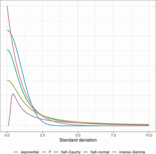
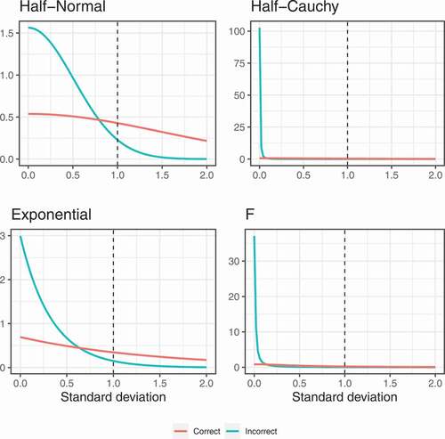
In this section, we compare the probability density functions of the various priors to better understand their behavior. shows the densities for the standard deviation. We use a scale of 1 for the robust priors and hyperparameters equal to 0.1 for the inverse-Gamma prior. The main difference between the inverse-Gamma prior and the more robust alternatives is that the inverse-Gamma prior has zero density at zero. As a result, the prior favors standard deviations that are away from 0, which is problematic, especially for standard deviations of random effects, which are often very close to 0. The inverse-Gamma prior thus automatically favors more complex models with less pooling. The other priors do have prior probability around standard deviations equal to zero and are therefore more in line with what we might expect in reality and are less likely to overfit.
Figure 2. Densities of the priors on the standard deviations
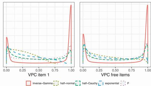
There are multiple standard deviations in the model for which a prior needs to be specified, specifically: ,
, and
. Together with the factor loadings at the between and within level,
and
, these standard deviations play a role in computing the VPC
for each item (see EquationEquation (6)
(6)
(6) ). As a result, specifying a prior on the standard deviations and factor loadings implies a certain prior on the VPC. This prior is considered in . Recall from Section 2.1 that we fixed the loading of one item to 1 for identification purposes. The left figure shows the VPC of the restricted item while the figure on the right shows the VPC of the unrestricted items. It is clear that this restriction has consequences for the implied prior of the VPC. This is due to the fact that the VPC depends on the loadings (see EquationEquation (6)
(6)
(6) ). Specifically, we see that some priors put less probability on a VPC close to 1 for the restricted item compared to the free items. This is most pronounced for the priors with the thinnest tails, that is, the half-normal and exponential priors. Furthermore, the implied priors on the VPC are not symmetrical. This is due to the fact that we assume a standard logistic distribution for the residuals at the within level. As a result,
, which arises in the denominator of EquationEquation (6)
(6)
(6) is fixed as well.
Figure 3. Densities of the implied priors on the variance partition coefficient (VPC) of the restricted and free items
Simulation studies
In order to investigate the performance of the robust priors for the random effects variances, we conduct two simulation studies. In the first study, we vary the population values for various parameters while keeping the number of groups fixed. We focus on comparing the traditional priors for variance parameters to a default setting of the more robust alternatives. In the second study, we use the same generated data sets as in the first study, but now we focus on informative prior settings with either correct or incorrect information to determine how robust the priors are to misspecifications. In both studies, we generate data according to the model in Section 2 using the following population values.
Population values for the variance parameters
The population value for the latent variable variance parameters is equal to 0.01 or 1. The sensitivity of the inverse-Gamma priors to the hyperparameter choice arises especially in situations in which the random effects variance is close to zero (Gelman, Citation2006). Depending on which value is specified for each variance parameter, the VPC will vary. Hedges and Hedberg (Citation2007) provide an overview of VPC values for educational achievement based on longitudinal surveys conducted in the United States. They found VPCs ranging from .03 to .3. These values are in line with VPCs used in other simulation studies of multilevel SEMs (Depaoli & Clifton, Citation2015; Helm, Citation2018; Zitzmann et al., Citation2016). Therefore, we consider several combinations of the population values for the variance parameters that result in VPCs within this range. Note that the VPC depends on the following parameters:
(see (6)). We fix the population values for
and
to 1, and
to
for all items. We consider different combinations of population values for the variances of the latent variables,
and
and subsequently compute
given these values and a VPC of .03 or .3. An overview of the different population values for the variance parameters and the resulting VPC is presented in .
Table 2. Overview population values for the variance parameters and variance partition coefficient
Population values for the contextual effect
When using group-mean centering, the contextual effect is defined as . Marsh et al. (Citation2009) provide three different standardized effect size measures that can be interpreted similarly to Cohen’s
. They recommend to use either one of the two more conservative effect sizes. Here, we rely on the second effect size in Marsh et al. (Citation2009) to define the population values for the regression coefficients at the between and within level. This effect size standardizes the contextual effect with respect to the total variance of self-concept at the within level, that is,
, and is defined as:
where denotes the contextual effect, which is equal to
in the case of group-mean centering, and
and
denote the standard deviations of the predictor at the between and within level, respectively. We consider a small negative standardized contextual effect and no contextual effect, that is,
. We choose these values such that we are able to investigate the power to detect a small contextual effect as well as the type 1 error rate. We fix
to 0.2 and
and
to 1 and compute the value for
to obtain the required standardized effect size. The resulting values are shown in .
Combinations of the various population values result in 16 different conditions (2 values values
values
values ES). We consider these 16 conditions for a balanced design with 20 groupsFootnote6 and a sample size of 20 within each group. We use 20 groups based on Hox et al. (Citation2012) who concluded that 20 groups are sufficient for multilevel SEM. Moreover, 20 groups are still feasible in terms of data collection. The sample size of 20 within each group is based on educational contexts in which this can be seen as a realistic size for a school class.
Study 1: Influence of population values
In the first study, we analyze the data sets using the traditional uniform prior and the inverse-Gamma prior with ε = .1, .01, .001 (denoted by: IG.1, IG.01, and IG.001, respectively) as well as the robust half-Normal (HNdef), half-Cauchy (HCdef), F (Fdef), and Exponential (EXPdef) priors. For the robust priors, we consider a default setting in which the scale equals , following a general recommendation often made for a robust default specification (see also Subsection 3.4).
Study 2: Influence prior misspecifications
In the second study, we focus on informative prior distributions. Specifically, we choose the prior scale in such a way that
, where
equals the population value under which that parameter was simulated. We consider two settings: in the “correct” informative prior (i.e., HNinf, HCinf, Finf, and EXPinf),
such that the resulting prior has sufficient probability around the population value. In the “incorrect” informative prior (i.e., HNinc, HCinc, Finc, and EXPinc), on the other hand,
such that the prior has only very little mass on the population value. Since we never know the true value in practice, it is important to consider this situation to assess the robustness of the various priors to possible misspecifications. In total, we consider eight different prior specifications (four types of priors
two settings) for 16 population conditions in Study 2. show the various informative prior densities used in the simulation study when the population value for the standard deviation equals 0.1 or 1, respectively. Note that the incorrect F prior specification is missing when the population standard deviation equals 0.1 since this setting resulted in a scale
of 0, whereas the scale should be positive. However, in order to be consistent across priors in specifying the incorrect setting, we did not consider an alternative specification that did result in a positive scale. All priors are more peaked around zero in the incorrect specification, and therefore have less prior mass around the true population value compared to the correct specification. It might appear that both the half-Cauchy and F priors have almost no prior mass around the true population value, but this is just a visual consequence of these priors being very spread out due to their heavy tails.
Figure 4. Prior densities for the informative specifications when the population value for the standard deviation equals 0.1
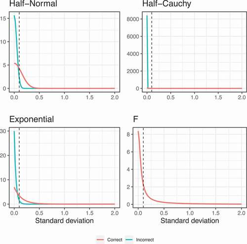
Figure 5. Prior densities for the informative specifications when the population value for the standard deviation equals 1
Outcomes
We consider the (relative) bias, mean squared error and 95% coverage rates,Footnote7 which are all computed based on the median estimate. The 95% coverage rates are computed based on the equal-tailed credible intervals which are defined by the 2.5% and 97.5% quantiles of the posterior distribution. We use 500 replications per condition and have computed the Monte Carlo SE for every outcome measure to quantify the uncertainty in the simulation results (Morris et al., Citation2019). All Monte Carlo SEs were sufficiently small to conclude that 500 replications were enough (the maximum MCSE was 0.03 for the coverage percentages).
All analyses were run using the R interface to Stan, RStan (Stan Development Team, Citation2018). The Hamiltonian Monte Carlo algorithm that is used in Stan converges much more quickly to the target distribution compared to, for example, Gibbs samplers (Hoffman & Gelman, Citation2014). As a result, less iterations are generally required to obtain sufficient independent samples of the posterior. For each analysis, we ran two MCMC chains with 3000 iterations each, half of which was used as burnin.Footnote8 We used a maximum treedepth of 10 and set adapt_delta to 0.90.
A replication is considered converged if the split (a version of the potential scale reduction factor, PSRF; Gelman and Rubin (Citation1992)) is smaller than or equal to 1.05 and there are no divergent transitions. If either one of these criteria is not met, that replication is removed from the results. For each condition, only the converged replications are used to compute the results and the results are only presented for those conditions in which there is at least 50% convergence (i.e., 250 converged replications). We also considered other, less strict convergence criteria, the results of which are available at https://osf.io/pq8gm/. We only report the results for
and
in cases where these variables did not have a substantial influence and refer to the online materials for the full results and tables on which the figures are based as well as all the code (https://osf.io/pq8gm/).
Results Study 1: Influence population values
Convergence
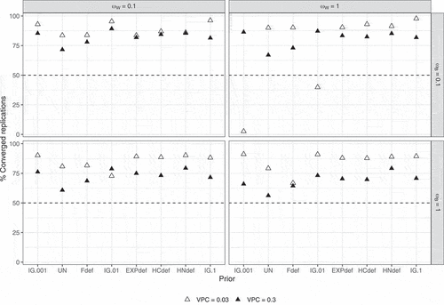
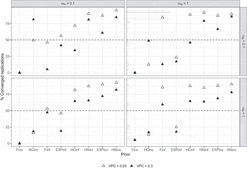
shows the percentages of converged replications for each prior, with dashed lines indicating 50% convergence. For , the inverse-Gamma prior sometimes showed substantially different convergence percentages. In general, the inverse-Gamma prior was most problematic with multiple conditions resulting in less than 50% convergence. With regard to the VPC, the smaller VPC of 0.03 generally led to higher convergence compared to the larger VPC of 0.3.
Figure 6. Percentages converged replications per condition according to the strict convergence criteria in Study 1 for
Bias
shows the relative bias, which can be multiplied by 100 to obtain a percentage, with the absolute bias in brackets for the variance parameters and the parameter of interest, . For the standard deviation of the latent variable at the between level,
, all priors resulted in some bias, although the values are comparable across most priors with the exception of the inverse-Gamma priors. Most priors underestimated
when the population value equals 1 and when the population value equals 0.1 combined with a VPC of 0.03. The IG(0.1, 0.1) prior, however, largely overestimated
when the population value equals 0.1, regardless of the value of the VPC. For the standard deviation of the latent variable at the within level,
, the robust priors showed only small biases when the population values equal 0.1, with more substantial underestimation when the population values equal 1, whereas the IG(0.1, 0.1) and IG(0.01, 0.01) priors showed a substantial overestimation when the population values equal 0.01. For the standard deviation of the items at the between level,
, we see a similar picture across all items. Specifically, the bias was generally small except for the IG(0.1, 0.1) prior when
and
. All priors underestimated the parameter of interest, the contextual effect
, regardless of the population condition. The relative bias was close to negative 100% when
equals 1 for all priors, but differed more across the priors when
equals 0.1.
Table 3. Relative bias (multiply by 100 to obtain percentages) with absolute bias in brackets for selected parameters based on strict convergence criteria and all converged replications in Study 1 for conditions in which
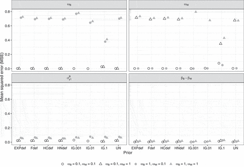
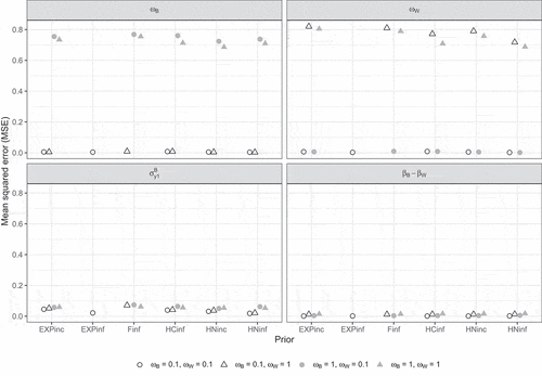
Mean squared error (MSE)
shows the MSE for selected parameters in Study 1. For both and
, lower population values for the corresponding parameter resulted in a smaller MSE. Differences between the priors are negligible, except for the IG(.1, .1) prior, which showed a smaller MSE compared to the other priors when the population value equals 1. For
, the MSE was slightly higher when
and when
(available online at: https://osf.io/pq8gm/) for all priors, while for the contextual effect, the MSE was close to zero across conditions and priors.
Figure 7. Mean squared error (MSE) per condition according to the strict convergence criteria in Study 1 for and
Coverage
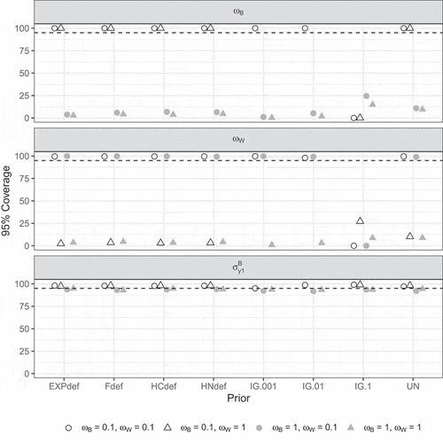
shows the 95% coverage rates for the selected parameters. For and
, coverage was much too low when the corresponding population values equal 1 and around 100% when the population values equal 0.1 for all priors except the IG(.1, .1) prior. Note that, for
, the coverage was higher when
and
(available online at: https://osf.io/pq8gm/), although it was still not close to the nominal 95% in this situation. For
, coverage was above the nominal 95% for all priors.
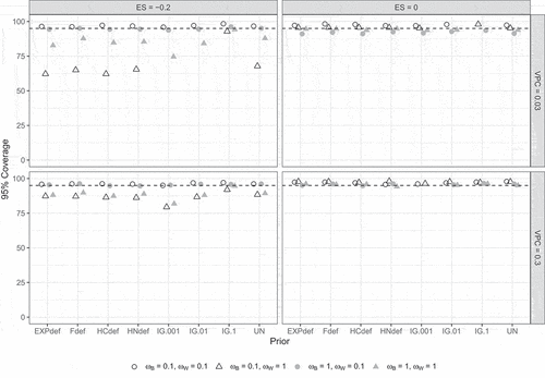
Figure 8. 95% coverage per condition according to the strict convergence criteria in Study 1 for and
and selected parameters. Dashed lines indicate the nominal 95%
shows the 95% coverage rates for the contextual effect . For this parameter, coverage rates depended on effect size and VPC. Specifically, coverage rates were too low when
(triangles) but only when
and not for the IG(.1, .1) prior.
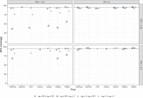
Figure 9. 95% coverage per condition according to the strict convergence criteria in Study 1 for the contextual effect . Dashed lines indicate the nominal 95%
Results Study 2: Influence prior misspecifications
We now turn to the results of the second simulation study in which we investigated the same population conditions as in Study 1, but with informative priors. The informative priors were specified such that they are either in line with the population values or not.
Convergence
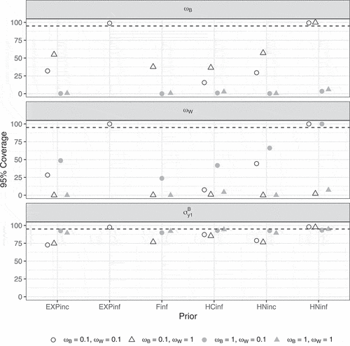
shows the percentages of converged replications for each prior in the second study. Again, only the results for are shown since the percentages for
were generally very similar, except for the correctly specified exponential prior (EXPinf). It is clear that, compared to the default priors in Study 1, the informative priors have more convergence problems. This is especially the case for the incorrectly specified F and half-Cauchy priors. For the incorrectly specified F prior, the convergence of 0% when at least one of the population standard deviations equals 0.1 is due to the fact that in these situations the prior scale equals zero whereas it should be positive (see also Subsection 3.7). Only the informative half-Normal priors and the incorrectly specified Exponential prior obtained more than 50% convergence in all conditions.
Figure 10. Percentages converged replications per condition according to the strict convergence criteria in Study 2 for
Bias
shows the relative bias with the absolute bias in brackets for the variance parameters and the parameter of interest, . As many conditions are missing due to non-convergence, it is difficult to compare the correctly and incorrectly specified informative priors. However, for the half-normal prior, the bias for
was lower for the correctly specified prior when
. Especially when the
, the difference between the correct and incorrect specifications was substantial. When
, the two specifications performed similarly. A similar picture arises for
, with the bias being lower for the correctly specified priors when the population value is small, and similar performance when the population value equals 1. For
, the biases were lower for the correctly specified half-normal prior across all population conditions, while the contextual effect
was underestimated across the board, regardless of the prior specification. Compared to the default half-normal prior in Study 1, the informative specification resulted in lower bias for
mainly when
and
, while in the other conditions the bias was comparable or slightly higher. For
, on the other hand, the default half-normal led to lower bias than the correct informative specification when
and comparable results otherwise.
Table 4. Relative bias (multiply by 100 to obtain percentages) with absolute bias in brackets for selected parameters based on strict convergence criteria and all converged replications in Study 2 for conditions in which
Mean squared error (MSE)
shows the MSE for selected parameters in Study 2. The results were very similar to those in Study 1 with negligible differences between the priors and mainly differences due to population values for the latent variable variance parameters, with higher population values (i.e., ) resulting in larger MSEs for the corresponding parameter.
Figure 11. Mean squared error (MSE) per condition according to the strict convergence criteria in Study 2 for and
Coverage
shows the 95% coverage rates for selected parameters in Study 2. Again, the coverage for and
was much too low when the corresponding population values equal 1 but, contrary to the coverage for the default priors (Study 1), the coverage remained too low for most priors when the population values equal 0.1, with the exception of the correctly specified exponential and half-normal priors. For
, coverage was close to the nominal 95% for all informative priors when
, but generally lower when
.
Figure 12. 95% coverage per condition according to the strict convergence criteria in Study 2 for and
and selected parameters. Dashed lines indicate the nominal 95%
shows the 95% coverage rates for the contextual effect . As in Study 1, coverage rates were close to the nominal 95% when
, but they were too low when
and
, especially when
.
Figure 13. 95% coverage per condition according to the strict convergence criteria in Study 2 for the contextual effect . Dashed lines indicate the nominal 95%
Discussion
The popularity of Bayesian MLSEM has inspired various investigations into the required number of groups (see, e.g., Depaoli & Clifton, Citation2015; Helm, Citation2018; Hox et al., Citation2012). However, these studies mainly rely on traditional default prior specifications, which have been proven to be unreliable, or correctly specified informative priors that are not feasible in practice. The goal of this study was to investigate more robust prior distributions for the random effects variances in the context of MLSEM. In order to do so, we have investigated default and (in)accurate informative prior specifications of popular robust prior distributions in a doubly latent categorical multilevel model.
The differences between the robust prior distributions and the uniform prior were generally small. The main differences in results in the simulation studies appear to arise due to the population conditions rather than the prior distribution. Only the inverse-Gamma specifications showed substantially different, and often worse, performance. The lack of differentiation in results between the robust priors and the uniform prior might be due to the simulated data sets being too large and thereby overruling the influence of the prior on the posterior distribution. It might be expected that in more extreme conditions, either in terms of a smaller number of groups or a smaller number of observations within each group, more substantial differences between the priors will arise. However, given the complexity of the model, we believe that more extreme conditions than the ones considered in this paper would not be realistic scenarios where such a model should be used.
The default specification for the robust priors did show bias for the random effects variance parameters as well as the parameter of interest, the contextual effect. The MSE of the random effects variance parameters was high in certain conditions but close to zero for the contextual effect across all conditions. The coverage for the random effects variance parameters was much too low but only low for the contextual effect in certain population conditions. These results indicate that, although the robust prior distributions are better options for the random effects variance parameter than the inverse-Gamma prior, their hyperparameters still require careful consideration in order to obtain the best results. This was further investigated in Study 2, where we considered (in)accurate informative specifications for the robust priors. Unfortunately, the informative priors resulted in low convergence percentages, which complicated a thorough investigation and comparison of their performance. Again, this illustrates the difficulty in specifying the hyperparameters for these robust prior distributions. Future research should further investigate these and other informative specifications to fully assess their robustness against misspecification.
One limitation of the simulation study lies in the fact that we removed the non-converged replications from the results. If the non-convergence in these removed replications is due to particular sample values, this approach might bias the simulations. We tried to partially remedy this problem by also considering weaker convergence criteria, which resulted in less non-converged replications but generally did not show substantial differences in terms of bias, MSE, and coverage. Still, non-convergence and how to deal with it remains an issue in any simulation study investigating extreme conditions in terms of sample size or population values. Compared to other MCMC algorithms, the Hamiltonian Monte Carlo algorithm used in Stan offers more convergence criteria. An advantage is that convergence can be assessed more accurately; however, it will also flag a replication as non-converged more easily. Especially for large models, such as the model considered here, a few divergent transitions can occur rapidly, resulting in a replication that is flagged as non-converged. It can therefore be useful to compare the results obtained using various convergence criteria.
Throughout this paper, we have focused on the prior for the random effects variance or standard deviation. In regular multilevel models, several authors have proposed to specify priors on the VPC, which leads to an implied prior on the random effects variance (see, e.g., Daniels, Citation1999; Gustafson et al., Citation2006; Mulder & Fox, Citation2018; Natarajan & Kass, Citation2000). Although we have considered specifying a prior directly on the VPC, this approach is not straightforward in MLSEM. Specifically, since the VPC depends on multiple other model parameters (see EquationEquation (6)(6)
(6) ), a choice needs to be made for which of those model parameters a prior is directly specified and for which of the model parameters the prior is implied. Future research is needed to investigate these choices and their consequences.
In this study, we have focused on the doubly latent categorical multilevel model, a popular multilevel SEM that is often used in practice. Even though some general principles apply regarding the sensitivity of the results to the prior distribution and we, thus, might expect some of the results found here to generalize to other multilevel structural equation models (such as the bad performance of the inverse-Gamma priors), the complexity of SEMs makes generalizations beyond the model considered here difficult. The complex interplay of parameters in SEMs, combined with the small amount of information on higher levels in multilevel models can result in possibly unexpected consequences of particular prior specifications. This illustrates the importance of understanding the behavior of the joint prior that a researcher specifies (e.g., through the use of prior predictive checks; Gabry et al., Citation2019) as well as conducting extensive prior sensitivity checks to investigate the sensitivity of the final results to the specified prior (Van Erp et al., Citation2018).
Bayesian MLSEM offers a powerful modeling framework to incorporate both measurement and sampling error within one model. However, the results presented in this paper indicate that some caution is warranted in applying these models. When the sample size is small, Bayesian estimation does not necessarily perform well (Smid et al., Citation2019). In order for Bayesian estimation to outperform classical estimation methods, the prior distribution needs to be well thought out. This is especially the case for the complex MLSEM considered in this paper: with only 20 groups, it is crucial for the prior distribution to add reasonable prior information to the analysis. More research is needed to investigate how we can achieve this.
Acknowledgments
We would like to thank Irene Klugkist, Duco Veen, and Mariëlle Zondervan-Zwijnenburg for helpful comments on an earlier version of this manuscript.
Additional information
Funding
Notes
1 Note that, generally, empirical data investigating the BFLPE, such as the PISA data (OECD, Citation2007), uses 4-point Likert scale indicators for academic self-concept. However, we assume binary indicators instead to keep the computation time feasible in our simulation studies.
2 Alternatively, a probit link function can be used, in which case .
3 These restrictions are, in theory, sufficient to identify the model. However, it is generally recommended to additionally impose cross-level invariance, that is, λW = λB to improve interpretability of the factors at both levels and to avoid estimation issues (Jak, Citation2018).
4 This corresponds to the parametrization used in Pérez et al. (Citation2017) when ,
, and
.
5 We parametrize the exponential distribution in terms of the scale for consistency, but generally it is defined using the rate parameter
, which is the inverse of the scale, that is,
.
6 A third simulation study investigated the influence of the number groups and analyzed a subset of conditions for 50 and 100 groups. However, as the number of groups increased, we ran into more convergence issues. Results for converged conditions are available online at https://osf.io/pq8gm/.
7 We also considered the power and type 1 error rates. However, power to find a small contextual effect was low across the board (ranging from 0.01 to 0.09 even for 50 groups) and type 1 error rates were around the nominal 5% for all conditions, so these results are only available online at https://osf.io/pq8gm/. Initially, we also compared the precision of the various priors through the empirical SE, which is computed as , with
denoting the mean of
. However, the empirical SE was sufficiently small in all conditions and for all priors (in the order of 1e-14) that we do not include this outcome in the results.
8 To assess the influence of the number of iterations on convergence, we reran one condition with 30,000 iterations per chain. However, this did not increase the convergence percentage or lead to substantial differences in the results. The results for this comparison are available at https://osf.io/pq8gm/.
References
- Asparouhov, T., & Muthen, B. (2007). Computationally efficient estimation of multilevel high-dimensional latent variable models. In Proceedings of the 2007 JSM meeting in Salt Lake City, Utah, section on statistics in epidemiology (pp. 2531–2535). Salt Lake City, Utah.
- Asparouhov, T., & Muthén, B. (2012). General random effect latent variable modeling: Random subjects, items, contexts, and parameters. http://www.statmodel.com/download/NCME12.pdf
- Asparouhov, T., & Muthén, B. (2019). Latent variable centering of predictors and mediators in multilevel and time-series models. Structural Equation Modeling, 26, 119–142. https://doi.org/10.1080/10705511.2018.1511375
- Berger, J. (2006). The case for objective bayesian analysis. Bayesian Analysis, 1, 385–402. https://doi.org/10.1214/06-BA115
- Berger, J. O., & Strawderman, W. E. (1996). Choice of hierarchical priors: Admissibility in estimation of normal means. The Annals of Statistics, 24, 931–951. https://doi.org/10.1214/aos/1032526950
- Daniels, M. J. (1999). A prior for the variance in hierarchical models. Canadian Journal of Statistics, 27, 567–578. https://doi.org/10.2307/3316112
- Depaoli, S., & Clifton, J. P. (2015). A bayesian approach to multilevel structural equation modeling with continuous and dichotomous outcomes. Structural Equation Modeling, 22, 327–351. https://doi.org/10.1080/10705511.2014.937849
- Frühwirth-Schnatter, S., & Wagner, H. (2010). Stochastic model specification search for gaussian and partial non-gaussian state space models. Journal of Econometrics, 154, 85–100. https://doi.org/10.1016/j.jeconom.2009.07.003
- Fúquene, J., Pérez, M.-E., & Pericchi, L. R. (2014). An alternative to the inverted gamma for the variances to modelling outliers and structural breaks in dynamic models. Brazilian Journal of Probability and Statistics, 28, 288–299. https://doi.org/10.1214/12-BJPS207
- Gabry, J., Simpson, D., Vehtari, A., Betancourt, M., & Gelman, A. (2019). Visualization in bayesian workflow. Journal of the Royal Statistical Society: Series A (Statistics in Society), 182, 389–402. https://doi.org/10.1111/rssa.12378
- Gelman, A. (2006). Prior distributions for variance parameters in hierarchical models (comment on article by Browne and Draper). Bayesian Analysis, 1, 515–534. https://doi.org/10.1214/06-BA117A
- Gelman, A., & Rubin, D. B. (1992). Inference from iterative simulation using multiple sequences. Statistical Science, 7, 457–472. https://doi.org/10.1214/ss/1177011136
- Ghosh, J., Li, Y., & Mitra, R. (2018). On the use of cauchy prior distributions for bayesian logistic regression. Bayesian Analysis, 13, 359–383. https://doi.org/10.1214/17-BA1051
- Goldstein, H., Browne, W., & Rasbash, J. (2002). Partitioning variation in multilevel models. Understanding Statistics, 1, 223–231. https://doi.org/10.1207/S15328031US0104_02
- Gustafson, P., Hossain, S., & Macnab, Y. C. (2006). Conservative prior distributions for variance parameters in hierarchical models. Canadian Journal of Statistics, 34, 377–390. https://doi.org/10.1002/cjs.5550340302
- Hedges, L. V., & Hedberg, E. C. (2007). Intraclass correlation values for planning group-randomized trials in education. Educational Evaluation and Policy Analysis, 29, 60–87. https://doi.org/10.3102/0162373707299706
- Helm, C. (2018). How many classes are needed to assess effects of instructional quality? A monte carlo simulation of the performance of frequentist and bayesian multilevel latent contextual models. Psychological Test and Assessment Modeling, 60, 265–285. https://www.psychologie-aktuell.com/fileadmin/download/ptam/2-2018_20180627/07_PTAM-2-2018_Helm_v2.pdf
- Hoffman, M. D., & Gelman, A. (2014). The no-u-turn sampler: Adaptively setting path lengths in Hamiltonian Monte Carlo. Journal of Machine Learning Research, 15, 1593–1623. https://www.jmlr.org/papers/volume15/hoffman14a/hoffman14a.pdf
- Hox, J. J., & Maas, C. J. M. (2001). The accuracy of multilevel structural equation modeling with pseudobalanced groups and small samples. Structural Equation Modeling, 8, 157–174. https://doi.org/10.1207/S15328007SEM0802_1
- Hox, J. J., Van de Schoot, R., & Matthijsse, S. (2012). How few countries will do? comparative survey analysis from a bayesian perspective. Survey Research Methods, 6, 87–93. https://ojs.ub.uni-konstanz.de/srm/article/view/5033
- Jak, S. (2018). Cross-level invariance in multilevel factor models. Structural Equation Modeling, 26, 607–622. https://doi.org/10.1080/10705511.2018.1534205
- Klein, N., & Kneib, T. (2016). Scale-dependent priors for variance parameters in structured additive distributional regression. Bayesian Analysis, 11(4), 1071–1106. https://doi.org/10.1214/15-BA983
- Lunn, D., Spiegelhalter, D., Thomas, A., & Best, N. (2009). The BUGS project: Evolution, critique and future directions. Statistics in Medicine, 28, 3049–3067. https://doi.org/10.1002/sim.3680
- Marsh, H. W., Lüdtke, O., Robitzsch, A., Trautwein, U., Asparouhov, T., Muthén, B., & Nagengast, B. (2009). Doubly-latent models of school contextual effects: Integrating multilevel and structural equation approaches to control measurement and sampling error. Multivariate Behavioral Research, 44, 764–802. https://doi.org/10.1080/00273170903333665
- Meuleman, B., & Billiet, J. (2009). A Monte Carlo sample size study: How many countries are needed for accurate multilevel SEM? Survey Research Methods, 3, 45–58. https://biblio.ugent.be/publication/1041001/file/6718903.pdf
- Morris, T. P., White, I. R., & Crowther, M. J. (2019). Using simulation studies to evaluate statistical methods. Statistics in Medicine, 38, 2074–2102. https://doi.org/10.1002/sim.8086
- Mulder, J., & Fox, J.-P. (2018). Bayes factor testing of multiple intraclass correlations. Bayesian Analysis, 14. https://doi.org/10.1214%2F18-ba1115
- Mulder, J., & Pericchi, L. R. (2018). The matrix-f prior for estimating and testing covariance matrices. Bayesian Analysis, 13, 1189–1210. https://doi.org/10.1214/17-BA1092
- Muthen, B. O. (1991). Multilevel factor analysis of class and student achievement components. Journal of Educational Measurement, 28, 338–354. https://doi.org/10.1111/j.1745-3984.1991.tb00363.x
- Muthén, B. O. (1994). Multilevel covariance structure analysis. Sociological Methods & Research, 22, 376–398. https://doi.org/10.1177/0049124194022003006
- Natarajan, R., & Kass, R. E. (2000). Reference bayesian methods for generalized linear mixed models. Journal of the American Statistical Association, 95, 227–237. https://doi.org/10.1080/01621459.2000.10473916
- OECD. (2007). PISA 2006. OECD.
- Pérez, M.-E., Pericchi, L. R., & Ramrez, I. C. (2017). The scaled beta2 distribution as a robust prior for scales. Bayesian Analysis, 12, 615–637. https://doi.org/10.1214/16-BA1015
- Piironen, J., & Vehtari, A. (2015). Projection predictive variable selection using stan+ r. arXiv preprint. arXiv:1508.02502.
- Polson, N. G., & Scott, J. G. (2012). On the half-cauchy prior for a global scale parameter. Bayesian Analysis, 7, 887–902. https://doi.org/10.1214/12-BA730
- Roos, M., Held, L. (2011). Sensitivity analysis in bayesian generalized linear mixed models for binary data. Bayesian Analysis, 6, 259–278. https://doi.org/10.1214/11-BA609
- Simpson, D., Rue, H., Riebler, A., Martins, T. G., & Sørbye, S. H. (2017). Penalising model component complexity: A principled, practical approach to constructing priors. Statistical Science, 32, 1–28. https://doi.org/10.1214/16-STS576
- Smid, S. C., McNeish, D., Miočević, M., & Van de Schoot, R. (2019). Bayesian versus frequentist estimation for structural equation models in small sample contexts: A systematic review. Structural Equation Modeling, 27, 131–161. https://doi.org/10.1080%2F10705511.2019.1577140
- Stan Development Team. (2015). Prior choice recommendations. Retrieved August 5, 2019, from https://github.com/stan-dev/stan/wiki/Prior-Choice-Recommendations
- Stan Development Team. (2018). RStan: The R interface to Stan. R package version 2.18.2. http://mc-stan.org/
- Van Erp, S., Mulder, J., & Oberski, D. L. (2018). Prior sensitivity analysis in default bayesian structural equation modeling. Psychological Methods, 23, 363–388. https://doi.org/10.1037/met0000162
- Yuan, Y., & MacKinnon, D. P. (2009). Bayesian mediation analysis. Psychological Methods, 14, 301–322. https://doi.org/10.1037/a0016972
- Zitzmann, S., Lüdtke, O., Robitzsch, A., & Marsh, H. W. (2016). A bayesian approach for estimating multilevel latent contextual models. Structural Equation Modeling, 23, 661–679. https://doi.org/10.1080/10705511.2016.1207179