Flexible Extensions to Structural Equation Models Using Computation Graphs

ABSTRACT

Structural equation modeling (SEM) is being applied to ever more complex data types and questions, often requiring extensions such as regularization or novel fitting functions. To extend SEM, researchers currently need to completely reformulate SEM and its optimization algorithm – a challenging and time–consuming task. In this paper, we introduce the computation graph for SEM, and show that this approach can extend SEM without the need for bespoke software development. We show that both existing and novel SEM improvements follow naturally. To demonstrate, we introduce three SEM extensions: least absolute deviation estimation, Bayesian LASSO optimization, and sparse high–dimensional mediation analysis. We provide an implementation of SEM in PyTorch – popular software in the machine learning community – to accelerate development of structural equation models adequate for modern–day data and research questions.

KEYWORDS:

• Structural equation modeling
• computation graphs
• deep learning
• optimization
• regularization

Introduction

Structural equation modeling (SEM) is a popular tool in the social and behavioral sciences, where it is being applied to ever more complex data types. For example, SEM extensions now perform variable selection in high–dimensional situations (Jacobucci et al., 2018; Van Kesteren & Oberski, 2019), modeling of intensive longitudinal data (Asparouhov et al., 2018; Voelkle & Oud, 2013),and analysis of intricate online survey experiments (Cernat & Oberski, 2019). In these situations, the SEM model often needs to be reformulated and traditional optimization approaches need to be extended to obtain parameter estimates—a challenging and time–consuming task. For example, applying SEM to high–dimensional data necessitates parameter penalization, and special model types such as genomic SEM (Grotzinger et al., 2019) or network models (Epskamp et al., 2017) can lead to alternative fitting functions. Additionally, even before the extension of SEM to novel data structures there have been several examples of the instability of the latent variable approach—such as Heywood cases (Kolenikov & Bollen, 2012) and convergence problems in multitrait–multimethod (MTMM) models (Revilla & Saris, 2013), which may benefit from regularization to obtain a stable result.

While the current growth of new types of structural equation models is exciting, developments in SEM are still far from caught up with the state–of–the–art in modern data analysis. In particular, the machine learning literature has exploded over the past decades to develop methods that deal with the complex nature of modern data, making great strides in difficult data analysis problems, including computer vision, natural language processing, and genomics (see Goodfellow et al., 2016, and the references therein for an overview). Each of these data sources holds great potential for research questions from the social, behavioral, ecological, or biomedical sciences where SEM is commonly used. However, traditional implementations of SEM are difficult to integrate with the modern data solutions pioneered in the field of machine learning.

In this paper, we propose allowing direct integration of SEM and methods from the field of deep learning, by specifying SEM as a computation graph. A computation graph is a representation of the mathematical steps needed to compute a loss function such as the likelihood. Because the graph allows for automatic differentiation, this computation graph can then not only be used to estimate the maximum likelihood estimates of SEM, but it can also be adjusted to incorporate penalties on specific parts of the SEM model, or to use a completely different loss function. We demonstrate the utility of our approach by straightforwardly implementing three potentially useful extensions to SEM, of which two are novel:

1. We implement Least Absolute Deviation (LAD) estimation, which exhibits robustness to outliers in the residual covariance matrix (Siemsen & Bollen, 2007).

2. To deal with high–dimensional indicators, we create a novel Bayesian LASSO estimation procedure (Park & Casella, 2008), and we apply it to an existing dataset to obtain a sparse linear combination of audio recording features related to Parkinson’s disease status at the latent variable level.

3. To analyze mediation models in which there are more potential mediators than rows, we develop a variant of sparse high–dimensional mediation analysis based on unweighted least squares (ULS). Using this method, we perform exploratory mediator selection in an epigenetic dataset (Schaid & Sinnwell, 2020; Van Kesteren & Oberski, 2019; Zhang et al., 2016).

These extensions are intended to demonstrate the power and flexibility of the proposed approach. The main purpose of this paper is to make this approach available to the SEM community to facilitate rapid development of novel extensions to SEM that will be useful in modern–day applications. To this end, we also provide an open source software package, tensorsem (https://doi.org/10.5281/zenodo.3957287).

This paper is structured as follows. First, SEM will be framed as an optimization problem, and a brief overview will be given of the current methods of SEM parameter estimation. Then, we will introduce the concept of computation graphs, as used in the field of deep learning. Subsequently, we will develop the computation graph for SEM, after which we show how this can be used to extend SEM to novel situations. Lastly, we discuss the implications of this novel framework for SEM and we provide directions for future research. The methods introduced this paper are implemented in open–source software, combining the popular R package lavaan (R Core Team, 2018; Rosseel, 2012) and the PyTorch neural network software (Paszke et al., 2019). All the examples associated with this paper are reproducible using the code in the supplementary material.

Background

SEM as an optimization problem

SEM in its basic form (Bollen, 1989) is a framework to model the covariance matrix of a set of observed variables. Through separation of structural and measurement models, it enables a wide range of multivariate models with both observed and latent variables. SEM generalizes many common data analysis methods, such as linear regression, seemingly unrelated regression, errors–in–variables models, confirmatory and exploratory factor analysis (CFA/EFA), multiple indicators multiple causes (MIMIC) models, instrumental variable models, random effects models, and more.

Below, we reiterate how the parameter configuration of the SEM framework creates a model–implied covariance matrix. Then, we show how this matrix is the basis for fitting functions representing the distance between the model–implied and the observed covariance matrix. Next, we show how such fitting functions are used to estimate the parameters of interest in the maximum likelihood (ML) and generalized least squares (GLS) frameworks.

The most commonly used formulations of SEM are the LISREL notation (Jöreskog & Sörbom, 1993) used in software packages such as lavaan (Rosseel, 2012) and the Reticular Action Model (RAM) notation (McArdle & McDonald, 1984) used in software such as OpenMX (Neale et al., 2016). In this paper, we adopt a variant of the LISREL notation known as the “all–y” version:

(1) $\begin{array}{cc}\mathit{z}& =\mathbf{\Lambda }\eta +\epsilon (\mathrm{M}\mathrm{e}\mathrm{a}\mathrm{s}\mathrm{u}\mathrm{r}\mathrm{e}\mathrm{m}\mathrm{e}\mathrm{n}\mathrm{t}\mathrm{m}\mathrm{o}\mathrm{d}\mathrm{e}\mathrm{l})\\ \eta & =B_0\eta +\mathit{\xi }(\mathrm{S}\mathrm{t}\mathrm{r}\mathrm{u}\mathrm{c}\mathrm{t}\mathrm{u}\mathrm{r}\mathrm{a}\mathrm{l}\mathrm{m}\mathrm{o}\mathrm{d}\mathrm{e}\mathrm{l})\end{array}$(1)

where $z$ represents a vector of centered observable variables of length $P$, and $\eta$, $\epsilon$, and $\xi$ are random vectors such that $\epsilon$ is uncorrelated with $\xi$ (Neudecker & Satorra, 1991). The parameters of the model are encapsulated in four matrices: $\mathbf{\Lambda }$ contains the factor loadings, $\mathbf{\Psi }$ contains the covariance matrix of $\mathit{\xi }$, ${\mathit{B}}_0$ contains the regression parameters of the structural model, and $\mathbf{\Theta }$ contains the covariance matrix of $\epsilon$. From these matrices, we construct the full parameter vector $\delta$ as follows:

(2) $\delta ={\left[{(\mathrm{v}\mathrm{e}\mathrm{c}\mathbf{\Lambda })}^T,(\mathrm{v}\mathrm{e}\mathrm{c}\mathrm{h}\mathbf{\Theta }{)}^T,(\mathrm{v}\mathrm{e}\mathrm{c}\mathrm{h}\mathbf{\Psi }{)}^T,(\mathrm{v}\mathrm{e}\mathrm{c}{B}_0{)}^T\right]}^T$(2)

where the $\mathrm{v}\mathrm{e}\mathrm{c}$ operator transforms a matrix into a vector by stacking the columns, and the $\mathrm{v}\mathrm{e}\mathrm{c}\mathrm{h}$ operator does the same but eliminates the supradiagonal elements of the matrix. Specific models impose specific restrictions on this parameter vector. This leads to a subset of free parameters $\theta$. $\delta$ is identified through predefined restrictions: $\delta =\delta (\theta )$. The model–implied covariance matrix $\sum (\theta )$ is a function of the free parameters, defined as follows (Bock & Bargmann, 1966; Jöreskog, 1966):

(3) $\sum (\theta )=\mathbf{\Lambda }{B}^{-1}\mathbf{\Psi }{B}^{-T}{\mathbf{\Lambda }}^T+\mathbf{\Theta }$(3)

where $B=I-B_0$ is assumed to be non–singular – that is, the structural path model $B_0$ is assumed to be identified.

In order to estimate $\theta$, an objective (“fitting”) function needs to be defined. All common SEM objectives are measures of the distance between the model–implied covariance matrix $\sum (\theta )$ and the observed covariance matrix $S$: the model fits better if the model–implied covariance matrix more closely resembles the observed covariance matrix. The maximum–likelihood (ML) objective function $F_{\mathrm{M}\mathrm{L}}$ is such a distance measure. Under the assumption that the observed covariance matrix follows a Wishart distribution or, equivalently, the observations follow a multivariate normal distribution, the maximum–likelihood (ML) fitting function is the following (Bollen, 1989; Jöreskog, 1967):

(4) $F_{\mathrm{M}\mathrm{L}}(\theta )=log\left|\sum (\theta )\right|+\mathrm{t}\mathrm{r}\left[\mathit{S}{\sum }^{-1}(\theta )\right]$(4)

Note that the ML fitting function is a special case of the generalized least squares (GLS) fitting function (Browne, 1974) which is defined as the following quadratic form:

(5) $F_{\mathrm{G}\mathrm{L}\mathrm{S}}(\theta )=(s-\sigma (\theta ){)}^{T}W(s-\sigma (\theta ))$(5)

Where $s=\mathrm{v}\mathrm{e}\mathrm{c}\mathrm{h}S$, and $\delta (\theta )=\mathrm{v}\mathrm{e}\mathrm{c}\mathrm{h}\sum (\theta )$. Here, $F_{\mathrm{G}\mathrm{L}\mathrm{S}}=F_{\mathrm{M}\mathrm{L}}$ when $\mathit{W}=2^{-1}{\mathit{D}}^T({\sum }^{-1}(\theta )\otimes {\sum }^{-1}(\theta ))\mathit{D}$ (Neudecker & Satorra, 1991), where $\mathit{D}$ is the duplication matrix and $\otimes$ indicates the Kronecker product. Other choices for $\mathit{W}$ lead to other estimators, such as unweighted least squares (ULS) or diagonally weighted least squares (DWLS).

With this formulation, the gradient $\mathit{g}\mathbf{(}\theta \mathbf{)}$ of $F_{\mathrm{G}\mathrm{L}\mathrm{S}}$ with respect to the parameters $\theta$ and the Hessian $H(\theta )$ – the matrix of second–order derivatives – were derived by Neudecker and Satorra (1991). These two quantities are the basis for standard errors, robust statistical tests for model fit (Satorra & Bentler, 1988), as well as fast and reliable Newton–type estimation algorithms (Lee & Jennrich, 1979). One such algorithm is the Newton–Raphson algorithm, where the parameter estimates at iteration $i+1$ are defined as the following function of the estimates at iteration $i$

(6) ${\theta }^{(i+1)}={\theta }^{(i)}-{\mathit{H}}^{-1}({\theta }^{(i)})\cdot \mathit{g}({\theta }^{(i)})$(6)

Together, the objective function and the algorithm comprise an estimator—a way to compute parameter estimates using the data. Note that this estimator is developed specifically for GLS estimation of SEM. With every extension to GLS, this work needs to be redone: a bespoke new estimator (fitting function, gradient, Hessian, and algorithm) needs to be derived and implemented.

Optimization problems as computation graphs

In this paper, we suggest implementing the SEM optimization problem as a computation graph, to leverage the advances of the deep learning field for extending the SEM framework. A computation graph is a graphical representation of the operations required to compute a loss or objective value $F(\theta )$ from (a vector of) parameters $\theta$ (Abadi et al., 2016). The full computation is split into a series of differentiable smaller computational steps. Each of these steps is represented as a node, with directed edges representing the flow of computation toward the final result. Because the nodes are differentiable, computing gradients of the final (or any intermediate) result with respect to any of its inputs is automatic. Gradients are obtained by applying the chain rule of calculus starting at the node of interest and moving against the direction of the arrows in the graph. Thus, computation graphs are not only a convenient way of representing an objective function in a computer, but they also immediately provide the derivatives (and second derivatives), which are necessary to optimize functions or estimate standard errors. For example, consider the familiar ordinary least squares objective for linear regression:

(7) ${\mathit{F}}_{\mathit{L}\mathit{S}}\mathbf{(}\beta )=\sum _i({\mathit{y}}_{\mathit{i}}-{\mathit{x}}_i\beta {)}^2=(\mathit{y}-\mathit{X}\beta {)}^T(\mathit{y}-\mathit{X}\beta )$(7)

The computation graph of this objective function can be constructed as in Figure 1. This figure represents the objective by “unnesting” the equation from the inside outward into separate matrix operations: first, there is a matrix–vector multiplication of the design matrix $\mathbf{X}$ with the parameter vector $\beta$. Then, the resulting $n\times 1$ vector $\stackrel{\mathbf{ˆ}}{\mathbf{y}}$ is subtracted elementwise from the observed outcome $\mathbf{y}$, and the result is squared, then summed to output a single squared error loss value $F_{\mathrm{L}\mathrm{S}}$. The nodes in a computation graph may represent scalars, vectors, matrices, or even three – and higher–dimensional arrays. Generally, these nodes are referred to as tensors.

Figure 1. Least squares regression computation graph, mapping the regression coefficients ($\beta$) to the least squares objective function $F_{\mathrm{L}\mathrm{S}}$. The gray parts contain elements which do not change as the parameters are updated, in this case observed data

Figure 2. Full computation graph for all–y structural equation model, mapping the parameters ($\delta$) to the maximum likelihood fit function $F_{\mathrm{M}\mathrm{L}}$. The gray parts contain elements which do not change during model fitting, meaning either observed data or constrained parameters. (NB: The constrained elements in this graph are not representative of a specific model)

Figure 3. Full SEM computation graph for the least absolute deviation (LAD) objective. Compared to the ML fit function, the last part of the graph contains different operations

Figure 4. $B_0$ LASSO computation graph with a pre–defined $\lambda$ tuning parameter

Figure 5. Factor analysis model used to generate data for comparing the least absolute deviation (LAD) estimator to the maximum likelihood (ML) estimator in tensorsem. Residual variances of the indicators were all set to 1

Figure 6. Model applied to the Parkinson’s data. Parkinson status is a binary variable, X1 – X22 are biologically–inspired features of the audio recording, normalized and standardized

Figure 7. Factor loadings (left panel) and factor scores (right panel) in the Parkinson’s disease dataset. All but 6 features are set to 0 when estimating the model using a Bayesian LASSO. Error bars are omitted for this method as the quadratic approximation is known to produce inconsistent confidence intervals in this case. The right panel shows that the LASSO factor scores exhibit very similar properties when compared to the ML factor scores despite the sparsity

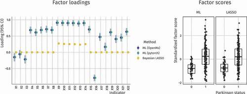
Figure 8. True and estimated indirect effects in a high–dimensional mediation analysis. The estimation methods are Unweighted Least Squares (ULS) and penalized ULS (LASSO). Regularized estimation correctly sets most parameters to 0 and shrinks the effect sizes overall

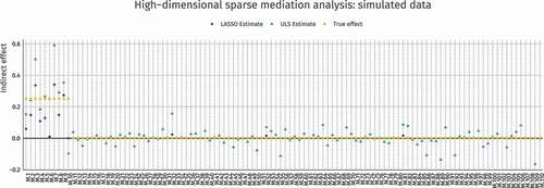
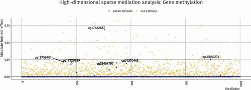
Figure 9. ULS and penalized ULS estimated absolute indirect effects in the Houtepen et al. (2016) dataset. Regularized estimation sets most parameters to 0 and shrinks the effect sizes overall, but for some mediators the effect sizes increase with penalization due to correlations among mediators. The top–5 strongest effect sizes are labeled, representing locations in the genome where mediation is strongest

Each of the operations in the graph has a registered derivative function. If it is known that the “square” operation $f(x)=x^2$ is applied as in Figure 1, the derivative $f{ }^{\mathrm{\prime }}(x)$ is $2x$ and the second–order derivative $f{ }^{\mathrm{\prime }}{ }^{\mathrm{\prime }}(x)$ is $2$. Thus, the gradient of the squared error tensor with respect to the residual tensor $r$ is $2r$.

Although automatic differentiation is an old idea (Wengert, 1964), its combination with state–of the art optimizers (see Appendix A) in software such as Torch (Collobert et al., 2002; Paszke et al., 2017) and TensorFlow (Abadi et al., 2016) have paved the way for the current pace of deep learning research. Before the development and implementation of the computation graph, each neural network configuration (model) required specialized work on the part of the researchers who introduced it to provide a novel estimator. Thanks to computation graphs, researchers can design generic neural nets without needing to invent a bespoke estimator. This development has greatly accelerated progress in this area. For SEM, we see a similar situation at the moment: each development or extension of the model currently requires a new algorithm that is capable of estimating its parameters. By applying computation graphs to SEM, we hope to greatly accelerate the process of developing novel SEM models. In the next section we combine the parameter configuration developed for SEM with the computation graphs and optimizers developed for deep learning to create a more flexible form of SEM.

Flexible extensions to SEM using computation graphs

In this section, we develop the computation graph and parameter configuration to perform default ML–based structural equation modeling using PyTorch (Paszke et al., 2019). Then, we outline how this computation graph can be edited to extend SEM to novel situations, and how additional penalties can be imposed on any parameter in the model. The last part of this section discusses obtaining standard errors in the computation graph approach to SEM. In the next section, we then show the flexibility of the computation graph approach described here by implementing and evaluating several useful extensions to traditional SEM.

The SEM computation graph

The SEM computation graph for the LISREL all–y notation is displayed in Figure 2. From left to right, a parameter vector $\delta$ is first instantiated with constrained elements, such that the free parameters represent $\theta$. Then, this vector is split into the separate vectors as in Equation (2)(2) $\delta ={\left[{(\mathrm{v}\mathrm{e}\mathrm{c}\mathbf{\Lambda })}^T,(\mathrm{v}\mathrm{e}\mathrm{c}\mathrm{h}\mathbf{\Theta }{)}^T,(\mathrm{v}\mathrm{e}\mathrm{c}\mathrm{h}\mathbf{\Psi }{)}^T,(\mathrm{v}\mathrm{e}\mathrm{c}{B}_0{)}^T\right]}^T$(2) . These vectors are then reshaped into the four SEM all–y matrices, using duplication indices for the symmetric matrices $\mathbf{\Psi }$ and $\mathbf{\Theta }$.

In the next part, these matrices are transformed to the model–implied covariance matrix $\sum (\theta )$ by unwrapping Equation (4)(4) $F_{\mathrm{M}\mathrm{L}}(\theta )=log\left|\sum (\theta )\right|+\mathrm{t}\mathrm{r}\left[\mathit{S}{\sum }^{-1}(\theta )\right]$(4) from the inside outward: $B^{-1}$ is constructed as $(I-B_0{)}^{-1}$, then $\mathbf{\Psi }$ is premultiplied by this tensor and postmultiplied by its transpose. Then, the resulting tensor itself is pre – and postmultiplied by $\mathbf{\Lambda }$ and ${\mathbf{\Lambda }}^T$, respectively. Lastly, $\mathbf{\Theta }$ is added to construct the implied covariance tensor.

The last part is the graphical representation of the ML fitting function from Equation (4)(4) $F_{\mathrm{M}\mathrm{L}}(\theta )=log\left|\sum (\theta )\right|+\mathrm{t}\mathrm{r}\left[\mathit{S}{\sum }^{-1}(\theta )\right]$(4) . $\sum (\theta )$ is inverted, then premultiplied by $S$, and the trace of this tensor is added to the log determinant of the inverse of $\sum (\theta )$. The resulting tensor, a scalar value, is the $F_{\mathrm{M}\mathrm{L}}(\theta )$ objective function for SEM.

Each operation in Figure 2 contains information about its gradient. PyTorch can therefore automatically compute gradients of the model parameters with respect to the fitting function in the SEM computation graph. The Hessian can also be obtained automatically by applying the same principle to the gradients. Note that these correspond to the observed score and information matrix, rather than their expected versions derived under the null hypothesis of model correctness. PyTorch also provides state–of–the–art optimizers such as Adam (Kingma & Ba, 2014) to optimize computation graphs using these quantities (see Appendix A for more background on these optimizers). The repository at https://doi.org/10.5281/zenodo.3957286 contains a software package which implements this computation graph, along with example code to estimate lavaan models using this package. Additionally, Appendix B shows that using the software we developed, it is possible to exactly replicate SEM analyses: in its basic implementation, the computation graph approach is equivalent to traditional SEM estimation approaches. Note that for specific models, additional optimization steps may be needed (see Discussion section for more).

Editing the objective function

The computation graph approach allows alternative objective functions to be implemented in SEM with relative ease. One such objective was coined by Siemsen and Bollen (2007), who introduce least absolute deviation (LAD) estimation. Their motivation is the performance of the LAD estimator as a robust estimation method in other fields. Note that while Siemsen and Bollen find limited relevance for this SEM estimator in terms of performance, we consider it to be an excellent showcase of the flexibility of our approach. This objective does not fit in the GLS approach of Browne (1974). The LAD estimator implies the following objective:

(8) ${\mathit{F}}_{\mathbf{L}\mathbf{A}\mathbf{D}}(\theta )=\sum _{i,j}\left|\sum {(\theta )}_{i,j}-{\mathit{S}}_{i,j}\right|$(8)

A computational advantage of this objective relative to the ML fit function is that there is no need to invert $\sum (\theta )$. The work of Siemsen and Bollen (2007) focuses on developing a greedy genetic evolution numerical estimation algorithm which performs a search over the parameter space. Using this optimization algorithm, they show that the LAD estimator may outperform the ML estimator in very specific situations.

Constructing the LAD estimator in the computation graph framework means replacing the ML fitting operations with the LAD operations. This is shown in Figure 3. Note that compared to the ML objective, there are fewer operations, and the inversion operation of the implied covariance matrix is removed. This change is trivial to make given the SEM computation graph, and we will show later in the Implementations section that such alternative objective functions can be estimated using PyTorch.

Adding parameter penalization

Another modification of default SEM is the addition of penalties to the parameters of structural equation models (Holmes Finch & Miller, 2020; P. H. Huang et al., 2017; Jacobucci et al., 2016). Such penalties regularize the model, which may prevent overfitting and improve generalizability (Hastie et al., 2015). There is a wide variety of parameter penalization procedures, but the most common methods are ridge and LASSO. In regression, the widely used elastic net (Zou & Hastie, 2005) is a combination of the LASSO and ridge penalties. The objective function for elastic net is the following:

(9) $F_{\mathrm{E}\mathrm{N}}(\beta )=F_{\mathrm{L}\mathrm{S}}(\beta )+{\lambda }_1{∥\beta ∥}_1+{\lambda }_2{∥\beta ∥}_1^2$(9)

where ${∥\beta ∥}_1={\sum }_p|{\beta }_p|$, and ${\lambda }_1$ and ${\lambda }_2$ are hyperparameters which determine the amount of LASSO and ridge shrinkage, respectively. By setting ${\lambda }_1$ to zero we obtain L2 (ridge) shrinkage, and setting ${\lambda }_2$ to zero yields the L1 (LASSO). Nonzero values for both parameters combines the two approaches, which has been shown to encourage a grouping effect in regression, where strongly correlated predictors tend to be in or out of the model together (Zou & Hastie, 2005).

Friedman et al. (2010) have developed an efficient algorithm for estimating the elastic net for generalized linear models and have implemented this in their package glmnet. For SEM, (Jacobucci et al., 2016) have created a package for performing penalization by adding the elastic net penalty to the ML fit function. Their implementation uses the RAM notation (McArdle & McDonald, 1984), and their suggestion is to penalize either the $A$ matrix (factor loadings and regression coefficients), or the $S$ matrix (residual covariances).

In the field of deep learning, parameter penalization is one of the key mechanisms by which massively overparameterized neural networks are estimated (Goodfellow et al., 2016). Regularization is therefore a core component of various software libraries for deep learning, including PyTorch. The optimizers implemented in these libraries, such as Adam (Kingma & Ba, 2014), are tried and tested methods for estimation of neural networks with penalized parameters, which is an active field of research (e.g., Scardapane et al., 2017).

In the SEM computation graph, the LASSO penalty on the regression parameters can be readily implemented by adding a few nodes to the ML fit graph. This is displayed in Figure 4. The absolute value of the elements of the $B_0$ tensor are summed, and the resulting scalar is multiplied by the tuning parameter. The resulting value is then added to the maximum likelihood fit tensor to construct the lasso objective $F_{\mathrm{L}\mathrm{A}\mathrm{S}\mathrm{S}\mathrm{O}}(\theta )$.

Ridge penalties for the $B_0$ matrix can be implemented in similar fashion, but instead of an “absolute value” operation, the first added node is a “square” operation. These penalties can be added to any tensor in the computation graph, meaning penalization of the factor loadings or the residual covariances, or even a penalty on $B$ is readily implemented. The elastic net penalty specifically can be implemented by imposing both a ridge and a lasso penalty on the tensor of interest.

Note that each additional penalty comes with its own parameter to be selected – a process called “hyperparameter tuning.” Tuning of penalty parameters is traditionally done through cross–validation; glmnet (Friedman et al., 2010) provides a function for automatically selecting the penalization strength in regression models through this method. Another method is through inspecting model fit criteria. For example, Jacobucci et al. (2016) suggest selecting the penalty parameter through the BIC or the RMSEA, where the degrees of freedom is determined by the amount of nonzero parameters, which changes as a function of the penalization strength. Another example is penalized network estimation, where Epskamp et al. (2018) suggest hyperparameter tuning through an extended version of the BIC. There is another option, used in both deep learning as well as Bayesian statistics: a prior can be set on the hyperparameters. In this way, the parameter itself is learned along with the model: the “full Bayes” approach (van Erp et al., 2019). In the deep learning literature, this is called Bayesian optimization or gradient–based optimization of hyperparameters (Bengio, 2000). In the Implementations section, we show how the Bayesian LASSO approach (Park & Casella, 2008) can be leveraged for sparse factor analysis in SEM, a completely novel extension.

Standard errors and model tests

In SEM, standard errors can be calculated through the Fisher information method, requiring only the Hessian of the log–likelihood at the maximum and the assumption that the distribution on which this log–likelihood is based (usually Normal–theory) is correct. Additionally, the distributional assumption can be relaxed by using sandwich estimators, in SEM known as Satorra–Bentler (robust) standard errors. These need both the Hessian and the $N\times P$ outer product matrix $\mathrm{\Delta }$ – the case–wise first derivatives of the parameters w.r.t. the implied covariances $\sigma (\theta )$ (Savalei, 2014). Sandwich estimators also lead to robust test statistics which are not sensitive to deviations from normality. In econometrics, many variations of the sandwich estimator are available, depending on whether the expected or observed information matrix is used (Kolenikov & Bollen, 2012).

Computation graphs as outlined in this section are a general approach for obtaining parameter estimates of structural equation models. Moreover, for the ML computation graph (Figure 2) it is also possible to obtain accurate standard errors because the observed information matrix – the inverse of the Hessian of the log–likelihood – is available automatically through the gradient computation in PyTorch. In addition, through the same computation graph but with case–wise entering of the data, the outer product matrix $\mathrm{\Delta }$ can also be made available. Because these are the observed versions, computation of empirical sandwich (Huber–White) standard errors is possible. Naturally, an established alternative to these procedures is to bootstrap in order to obtain standard errors. Furthermore, the log–likelihood itself is directly available, thus information criteria such as AIC, BIC and SSABIC (Sclove, 1987), as well as normal–theory and robust test statistics (Satorra & Bentler, 1988) can be computed more or less “as usual.”

In principle, therefore, standard errors and test statistics are available when using the computation graph approach. However, in practice the computation graph can be edited arbitrarily by introducing penalties or a different objective function. In this case, no general guarantees can be given about the accuracy of the standard errors, the coverage probability of the confidence interval, or the asymptotic behavior of model fit metrics derived from the obtained model. This is inherent to the flexibility of the computation graph approach: for existing methods in SEM, simulations have shown the performance of the current standard error solutions (including the bootstrap), but as extensions are introduced these results do not necessarily hold. For some extensions, there will be no adequate approximation to the standard error with accurate frequentist properties. For example, there is a large body of literature on standard error approximations for $L1$ penalization (e.g., Fan & Li, 2001), but the problem of obtaining penalized model standard errors is fundamentally unsolvable due to the bias introduced by altering the objective function away from the log–likelihood (Goeman et al., 2018, p. 18). Not even the bootstrap can provide consistent standard error estimates in these situations (Kyung et al., 2010). Hence, software implementations of penalized regression (e.g., glmnet) consciously omit standard errors.

In situations beyond ML, our advice is to pay attention to the behavior of existing fit criteria and standard errors. Using simulations for each new model and data case, the frequentist properties of the empirical confidence interval can be assessed and the type–I and type–2 errors of the (Satorra–Bentler) ${\chi }^2$ test can be found. Those values can then be used to adjust the interpretation of the results in the analysis of the real data. If existing standard error approaches fail altogether, a viable solution may be to completely omit standard errors—just as in the $L1$ regression approach.

Note that all of the above holds similarly for Bayesian estimation, where the choice of prior influences the frequentist properties of the posterior, such as the credible interval coverage probability. Just as it is possible with the computation graph approach to create a nonconverging model with bad asymptotic behavior, it is possible with Bayesian methods to create such a problematic model through the choice of nonsensical priors. Solutions in this case are also based on simulation, e.g., prior predictive checking (Gabry et al., 2019) or leave–one–out cross–validation (Vehtari et al., 2017).

In the next section, we show through a set of examples motivated by existing literature how our implementation of the SEM computation graph can be used to create extensions such as the ones we have introduced in this section.

Implementations

In this section, we implement three completely novel estimation procedures for SEM using our computation graph approach. The first example demonstrates how non–standard extensions to the fit function can be implemented with relative ease: we show how the Least Absolute Deviation (LAD) estimator yields similar parameters to the ML estimator in a factor analysis, even when the covariance matrix is contaminated with wrong values. Then, we perform a structural equation model with a sparse factor, using full Bayesian LASSO regularization (Park & Casella, 2008) for the factor loadings. To our knowledge, the full Bayesian optimization approach with hyperpriors has not previously been performed in the context of factor analysis with a covariate. Then, we perform high–dimensional mediation analysis with ULS optimization and LASSO regularization, using sparsity to select relevant variables among a set of 110 potential mediators. This procedure is also novel, and through our approach it can be implemented relatively simply.

All the computation graphs and estimation methods described in this paper are reproducible through the code in the supplementary material, as well as the R and python packages available at https://doi.org/10.5281/zenodo.3957287. Prior to implementing these examples, we have checked the validity of our PyTorch implementation for default and regularized SEM against several other packages. The results of this are shown in Appendix B.

LAD estimation

Although LAD estimation was shown to be beneficial only in very specific situations (Siemsen & Bollen, 2007), it is an excellent showcase for the flexibility of the computation graph approach. Because the software developed by Siemsen and Bollen (2007) is not available, we instead compare the LAD estimates to the ML estimates. The PyTorch LAD estimator is a completely novel way of estimating SEM.

For this example, we generate data of sample size 1000 from a one–factor model. For this data, we constrain the observed covariance matrix to the covariance matrix implied by the population model in Figure 5. Since LAD estimation should be robust to outliers in the observed covariance matrix, which can happen in the trivial case of mistranscribing a covariance matrix into software, we also performed this on data with a “contaminated” covariance matrix: $COV(X_1,X_3)=2,COV(X_2,X_4)=0.35$.

The results are shown in Table 1. The ML estimates in lavaan and tensorsem again agree. With the uncontaminated covariance matrix, the LAD estimates reach the same conclusion as the ML estimates. Note that although unbiased, LAD is relatively less efficient, but this effect is not visible with a sample size of 1000 for this model. With contamination in the covariance matrix, the LAD method shows no bias, whereas the ML method does. Because the Hessian for the LAD objective is not invertible, the standard errors are not available using the previously described $\mathrm{A}\mathrm{C}\mathrm{O}\mathrm{V}(\theta )$ method. Siemsen and Bollen (2007) solve this problem by bootstrapping, which is possible but outside the scope of the current paper.

Table 1. Parameter estimates comparing ML estimates to LAD estimates using both uncontaminated (u, top) and contaminated (c, bottom) covariance matrices. LAD is robust to the contamination of the covariance matrix

	X1	X2	X3	X4	X5	X6	X7	X8	X9
Uncontaminated (ML)	1.00	1.17	1.18	1.36	1.40	1.42	1.34	1.23	0.89
Contaminated (ML)	1.00	0.93	1.15	1.10	1.22	1.24	1.17	1.07	0.78
Uncontaminated (LAD)	1.00	1.17	1.18	1.36	1.40	1.42	1.34	1.23	0.89
Contaminated (LAD)	1.00	1.17	1.18	1.36	1.40	1.42	1.34	1.23	0.89

The results from this example show that the objective function in PyTorch can be edited and that Adam still converges to a stable solution with this adjusted objective. The parameter estimates from LAD estimation approximate those obtained from ML estimation in a one–factor model with 9 indicators and 1000 observations. In addition, we have observed that LAD estimation is robust to contamination of the covariance matrix in the contrived example of this section. Note that SEM estimation can be made robust against outliers in the raw data through using a multivariate $t$ likelihood (Asparouhov & Muthén, 2016; Lai & Zhang, 2017; Yuan & Bentler, 1998), which is possible in the computation graph approach but outside the scope of the current paper.

Sparse factor SEM

Obtaining sparsity in factor analysis is a large and old field of research, with methods including rotations of factor solutions in principal component analysis (Kaiser, 1958) and modification indices in CFA (Saris et al., 1987; Sörbom, 1989). Sparsity is desirable in factor analysis due to the enhanced interpretability of the obtained factors. Recently, penalization has been applied to different factor analysis situations in order to obtain sparse factor loadings and simple solutions (Choi et al., 2010; Jin et al., 2018; Lu et al., 2016; Pan et al., 2017; Scharf & Nestler, 2019). In addition, traditional factor rotations have been combined with SEM in a unified framework called exploratory SEM (ESEM, Asparouhov & Muthén, 2009). Several implementations of factor loading regularization now exist in SEM (e.g., Guo et al., 2012; P. H. Huang et al., 2017; Jacobucci et al., 2016).

Following these recent developments, in this example we impose sparse structure in a factor by imposing a penalty on the relevant elements of the $\mathbf{\Lambda }$ matrix. We reuse the example of Choi et al. (2010), who created a new lasso estimator for factor analysis and tested their method on an open Parkinson dataset. The example dataset is taken from the UCI Machine Learning repository (Dua & Graff, 2017) and is based on 195 voice recordings of people with and without Parkinson’s disease. Certain biologically inspired features (Little et al., 2007) of these audio recordings can be related to the disease status of the participants. In this example, we seek to find a sparse linear combination of these features which can be explained by the disease status. Note that this feature–based representation is similar in idea to Guo et al. (2012), who used Bayesian LASSO to select among basis functions, creating non–linear spline relations between latent variables and their indicators.

The model applied to the data is shown in Figure 6. After standardization and log–transforming the skewed features (see supplementary material for the full pre–processing pipeline), ML estimates for this model were obtained using standard SEM software (OpenMx; Neale et al., 2016, NB: lavaan’s optimization reached a local minimum), as well as via our PyTorch implementation. Then, a Bayesian LASSO penalty was added to the model: the objective function was equal to the ML fit function (Equation 4(4) $F_{\mathrm{M}\mathrm{L}}(\theta )=log\left|\sum (\theta )\right|+\mathrm{t}\mathrm{r}\left[\mathit{S}{\sum }^{-1}(\theta )\right]$(4) ) plus a Laplace prior on the factor loadings with a $Gamma(1.78,1)$ hyperprior on the scale of the double exponential distribution (Park & Casella, 2008). The resulting factor loadings and factor scores are shown in Figure 7.

The figure shows that the factor scores exhibit very similar class separation, despite the sparsity of the LASSO solution. In other words, using fewer features, a similar amount of information about the disease status is encoded in this factor. In this example, variable selection is informed by the disease status variable. The penalty parameter is learned automatically, along with the remaining variables. Furthermore, in this framework it is easy to extend the penalty to adaptive LASSO, where the strength of penalization is determined on a per–feature basis (Guo et al., 2012), or any of the myriad of alternative penalty functions, some of which are known to exhibit less bias in the nonzero parameters than the LASSO (Van Erp et al., 2019).

Sparse high–dimensional mediation

In this last example, we implement high–dimensional mediation analysis. This procedure is becoming more relevant as high–dimensional data becomes accessible due to reductions of cost and increasing availability of complex measurement devices. The motivating example for this high–dimensional mediation procedure can be found in Houtepen et al. (2016) and Van Kesteren and Oberski (2019): childhood trauma scores of participants were measured using a standard questionnaire, and their reactivity to stress later in life was measured using their cortisol patterns after a stressor. Gene methylation was measured for each participant and hypothesized to mediate the relation between childhood trauma and stress reactivity. The goal of this study was to identify locations in the genome where methylation has an influence on the relation between childhood trauma and stress reactivity, as a potential target for future research.

Crucially, ML estimation is not available with high–dimensional data, where the parameters outnumber the rows in the dataset, because the model–implied covariance matrix is not invertible. However, other analysis methods such as LAD estimation (Section 4.1) and ULS estimation do not need to invert the model–implied covariance matrix to obtain parameter estimates. In this section we use ULS estimation with a LASSO penalty on the paths. In this way, we perform variable selection among the mediators, while taking into account potential residual correlations between the mediators.

To test our approach, we have simulated a dataset following the same pattern as the motivating example. It contains 110 potential mediators, of which only 10 are true mediators with an indirect effect of .25. There are only 40 rows, making the dataset high–dimensional (for more details on data generation, see Van Kesteren & Oberski, 2019). Using this data, two mediation models were fit in PyTorch, one with only the ULS loss function, and one with the ULS loss function plus the sum of the absolute values of the indirect paths:

$L(\theta )=(s-\sigma (\theta ){)}^T(s-\sigma (\theta ))+\sum _{p\in P}|a_p|+\sum _{p\in P}|b_p|$

where $s$ and $\sigma (\theta ))$ are the half–vectorized observed and implied covariance matrix elements, $P$ is the total number of mediators, $a_p$ is the regression path from the predictor to the $p^{th}$ mediator, and $b_p$ is the regression path from the $p^{th}$ mediator to the outcome. Note that for simplicity, we have not included a multiplicative penalty hyperparameter, but this could be included in future implementations.

The true indirect effects ($a_p{b}_p$) and their estimates are shown in Figure 8. The penalization procedure correctly sets most mediation paths to 0, thus excluding their respective mediators from consideration. If we use this exclusion as a decision rule for variable selection, we obtain one false negative (M.10) and three false positives (M.32, M.52, and M.81), resulting in a respectable positive predictive value (PPV) of 75%.

Applying the same approaches, ULS and penalized ULS estimation, to 1000 preselected mediators from the real dataset (N = 85) from the motivating example yields the result shown in Figure 9. The top–5 most relevant locations are labeled using their methylation site identifier. This type of penalization approach can be valuable in discovering potential mediation targets for future research, and although a similar procedures have been implemented using LASSO on the $b_p$ paths (Y. T. Huang & Pan, 2015), LASSO on both $a_p$ and $b_p$ paths (Serang et al., 2017), or a group LASSO penalty (Schaid & Sinnwell, 2020), it has never been implemented using ULS estimation.

Together, the implementations have shown that estimation and extension of SEM through computation graphs and the Adam optimizer is viable. In a single unified optimization framework, we have implemented several extensions, either suggested in previous literature or completely novel. As previously mentioned, the exact properties of the novel procedures introduced here should be further analyzed in future work for different types of models. This is not the goal of the present work, where these examples have served as an illustration of the flexibility and viability of the computation graph approach in principle.

Conclusion

Estimation of SEM becomes more challenging as latent variable models become larger and more complex. Traditionally, SEM optimizers have already suffered from nonconvergence and inadmissible solutions (e.g., Chen et al., 2001; Revilla & Saris, 2013), and with the increasing complexity of available datasets these problems are set to become more relevant. We argue that current estimation methods do not fulfil the needs of researchers applying SEM to novel situations in the future.

In this paper, we have introduced a new way of constructing objective functions for SEM by using computation graphs. When combined with a modern optimizer such as Adam, available in the software package PyTorch, this approach opens up new directions for SEM estimation. The flexibility of the computation graph lies in the ease with which the graph is edited, after which gradients are computed automatically and optimization can be performed without in–depth mathematical analysis. This holds even for non–convex objectives and objectives which are not continuously differentiable, such as the LASSO objective. We have shown that previously proposed improvements to SEM, such as LAD estimation (Siemsen & Bollen, 2007), follow naturally from this framework, and that our implementation is able to optimize these, yielding parameter estimates that behave according to expectations. In addition, we demonstrated the ease with which extensions can be investigated by implementing a fully Bayesian LASSO and performing high–dimensional variable selection with the ULS loss and a LASSO penalty, both novel penalization methods for SEM.

While our approach is general and flexible, there might be faster or more stable solutions for estimating certain specific models. Software created for specific use–cases may use optimization tricks that are suited to a single type of model, which cannot possibly be incorporated in such a general procedure. For example, the Latent Gold software has been built specifically for estimating latent class models. It uses an EM algorithm to start the estimation procedure, and then performs Newton–Raphson optimization to move toward the final parameter estimates (Vermunt & Magidson, 2013, sec. 7.4). Such specific procedures are not available by default with our approach. To develop extensions, we suggest first checking whether the computation graph approach works well enough for the specific model of interest, and only then editing the graph toward the desired end–result.

As the computation graph approach paves the way for a more flexible SEM, researchers can use it to develop theoretical SEM improvements. For example, future research can focus on how penalties may be used to improve the performance and interpretability of specific models (e.g., Jacobucci et al., 2018) or how different objective functions may be used to bring SEM to novel situations such as high–dimensional data (Grotzinger et al., 2019; Van Kesteren, 2020). A potential extension to SEM is the use of high–dimensional covariates to debias inferences in observational studies (Athey et al., 2018). The computation graph may aid in importing such procedures to SEM. An interesting historical note is that Cudeck et al. (1993) have had similar reasons for creating a general SEM optimization program, where the full Hessian is numerically approximated for any covariance model and the solution is computed using Gauss–Newton iterations. The modern computational tools used here now make such generic SEM programs feasible.

Another topic for future research is exploratory model specification. For example, Brandmaier et al. (2013) and Brandmaier et al. (2016) use decision trees to find relevant covariates in SEM, and Marcoulides and Drezner (2001) use genetic algorithms to perform model specification search. Penalties provide a natural way to automatically set some parameters to 0, which is equivalent to specifying constraints in the model. A compelling example of this is the work by Pan et al. (2017), who used the Bayesian form of LASSO regularization as an alternative to post–hoc model modification in CFA. Their approach penalizes the residual covariance matrix of the indicators, leading to a more sparse selection of residual covariance parameters to be freed relative to the common modification index approach.

There is an opportunity for the SEM computation graph approach to be further developed to expand its range of applications. For example, through applying Adam as a stochastic gradient descent (SGD) optimizer it may be extended to perform full information maximum likelihood (FIML) estimation, batch–wise estimation, or SEM estimation with millions of observations. This will potentially enable SEM to be performed on completely novel types of data, such as streaming data, images, or sounds. Another improvement which may be imported from the deep learning literature is computation of approximate Bayesian posterior credible intervals for any objective function using stochastic gradient descent steps at the optimum (Mandt et al., 2017). The deep learning optimization literature moves fast, and through the connections we have established in this paper the SEM literature could benefit from its pace.

Acknowledgments

We thank Rogier Kievit and Laura Boeschoten for their comments on earlier versions of this manuscript and Maksim Rudnev for his helpful questions regarding our software.

Supplemental data

Supplemental data for this article can be accessed on the publisher’s website

Disclosure statement

No potential conflict of interest was reported by the author(s).

Additional information

Funding

This work was supported by The Netherlands Organization for Scientific Research (NWO) under grant number [406.17.057].

Appendix A.

Adaptive first–order optimizers

We suggest using adaptive first–order optimizers to extend SEM beyond the existing estimation methods. Adaptive first–order optimizers are a class of optimization algorithms designed to work even under nonconvexity and nonsmoothness. Some early algorithms such as RMSProp (Tieleman & Hinton, 2012) were originally developed with deep learning in mind, where nonconvexity, non–smoothness, and high–dimensional parameter spaces are common. Therefore, we consider these methods excellent candidates for estimating an expanding class of SEM models, as they have historically done for neural networks. The idea of using first–order optimizers for SEM is by no means new (Lee & Jennrich, 1979), but the recent developments in this area have made it a feasible approach.

The simplest first–order optimizer is gradient descent, which uses the gradient $g(\theta )$ of the objective with respect to the parameters to guide the direction that each parameter should move toward. The gradient is combined with a step size $s$ so that in each iteration $i$ of gradient descent the parameters are moved a small amount toward the direction of the negative gradient evaluated at the current parameter values:

(10) ${\theta }^{(i+1)}={\theta }^{(i)}-s\cdot g({\theta }^{(i)})$(10)

This algorithm has a similar structure to the Newton–Raphson method shown in Equation (6)(6) ${\theta }^{(i+1)}={\theta }^{(i)}-{\mathit{H}}^{-1}({\theta }^{(i)})\cdot \mathit{g}({\theta }^{(i)})$(6) . In that algorithm, the step size $s$ in each iteration is replaced by the inverse of the Hessian matrix. Gradient descent is thus a simplified version of the methods currently in use for optimizing SEM. Because it does not use the Hessian, it continues to function when the objective is not smooth or not convex. Computationally, it is also more tractable, foregoing the need to compute the full Hessian matrix. However, it is necessary to determine the correct step size $s$. This is not a trivial problem: with an improperly tuned step size, the algorithm may never converge.

One of the state–of–the art adaptive first–order optimizers is Adam (Kingma & Ba, 2014). It introduces two improvements to the framework of gradient descent (Figure A1). Firstly, it introduces momentum, where the direction in each iteration is not only the negative gradient of that iteration, but a moving average of the entire history of gradients. Momentum allows Adam to move through local minima in the search for a global minimum by smoothing the path it takes in the parameter space. Secondly, Adam introduces a self–adjusting step size for each parameter, which is adjusted based on the variability of the gradients over time: if the variability of the gradient of a parameter is smaller, Adam will take larger steps as it has more certainty about the direction the parameter should move in (and vice versa). This self–adjusting step size takes the place of computing and inverting the Hessian matrix. By using both the first and second moments of the history of the gradients, Adam is an adaptive optimizer capable of reliably optimizing a wide variety of objectives.

A relevant parallel to the development of adaptive first–order optimizers for deep learning is the recent advances in Bayesian SEM (Merkle & Rosseel, 2015) and Bayesian posterior sampling in general. Here, too, the objective function may be nonconvex, e.g., in hierarchical models and with nonconjugate priors. Such objective functions may lead to inefficient behavior for the Markov Chain Monte Carlo (MCMC) methods used to approximate posterior expectations. For this problem, Hamiltonial Monte Carlo (HMC) (Betancourt, 2017) has been developed, which introduces momentum in the proposal of a sample, thereby more efficiently exploring the posterior. This is the method implemented in Stan (Carpenter et al., 2017), which works for situations with many parameters and hyperparameters.

Adaptive first–order optimizers are one part of a pair of improvements that have enabled rapid growth of the deep learning field. The other is the development of computation graphs, an intuitive way of specifying the objective such that gradients can be computed automatically. Automatic gradient computation can enable a wide range of extensions to SEM without having to analytically derive the gradient and Hessian for each separate extension. In the next section, we explain the concept behind computation graphs and how they can be combined with optimizers such as Adam.

Figure A1. Three first–order algorithms finding the minimum of $F(\theta )={\theta }_1^2+5{\theta }_2^2$ with starting value $\hat{\theta }=[-0.9,-0.9]$. Gradient descent uses the gradient and a fixed step size ($s=0.01$) to update its parameter estimates. Gradient descent with momentum instead uses an exponential moving average of the gradients (decay of 0.9) with the same $s$. Finally, Adam adds a moving average of the squared gradient (decay of 0.999) to adjust the step size per parameter, leading to a straight line to the minimum with an overshoot and return due to momentum. In this example, Adam converges fastest, and gradient descent is slowest

Appendix B.

PyTorch estimation validation

B.1 ML–SEM estimation

We first validated our PyTorch implementation of default SEM through comparing the parameter estimates and their standard errors to two example models from the lavaan package: the Holzinger–Swineford model and the Political Democracy model. For more information about these models, see Rosseel (2012). The reproducible code for these models can be found in the supplementary material. The results are shown in Figure B1.

Figure B1. Comparison of parameter estimates and their 95% confidence interval for the Holzinger–Swineford and Political Democracy models. The plots show that both methods arrive at the same solution

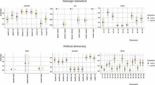
From this validation, we conclude that computation graphs and Adam optimization are together capable of estimating structural equation models. In addition, as the solution obtained by PyTorch is the same as with other packages, it is possible compute the value of the log–likelihood objective function and its derivative fit measures such as ${\chi }^2$, AIC, and BIC.

B.2 LASSO regularization

In this example, we show how LASSO penalization on the regression parameters in tensorsem compares to regsem (Jacobucci et al., 2016) and glmnet (Friedman et al., 2010). For this, we generate data with a sample size of 1000 from a regression model with a single outcome variable, 10 true predictors, and 10 unrelated variables. The resulting parameter estimates for the three different estimation methods are shown in Table B1. The table shows that with the chosen penalty parameter (0.11 for regsem and PyTorch, 0.028 for glmnet due to a difference in scaling), the estimates are very close in value. As expected, some parameters are shrunk to 0 for all three methods.

Table B1. Regularization with glmnet, regsem, and PyTorch. Table indicates parameter estimates for a LASSO penalized regression model with 20 predictors. PyTorch is compared to existing approaches and shown to provide similar parameter estimates. (dot indicates 0)

	1	2	3	4	5	6	7	8	9	10	11	12	13	14	15	16	17	18	19	20
glmnet	.	.07	.10	.07	.20	.23	.34	.13	.31	.17	–.03	.02	.05	.	.	.	.	.	.	.
regsem	.	.07	.10	.08	.20	.23	.34	.13	.31	.17	–.03	.02	.05	.	.	.	.	.	.	.
PyTorch	.	.07	.10	.07	.20	.23	.34	.13	.31	.17	–.03	.02	.05	.	.	.	.	.	.	.

References

- Abadi, M., Barham, P., Chen, J., Chen, Z., Davis, A., Dean, J., Devin, M., Ghemawat, S., Irving, G., Isard, M., & Kudlur, M. (2016). Tensorflow: A system for large–scale machine learning. 12th {USENIX} symposium on operating systems design and implementation ({OSDI} 16) (pp. 265–283).
- Asparouhov, T., Hamaker, E. L., & Muthén, B. (2018). Dynamic structural equation models. Structural Equation Modeling, 25, 359–388. https://doi.org/https://doi.org/10.1080/10705511.2017.1406803
- Asparouhov, T., & Muthén, B. (2009). Exploratory structural equation modeling. Structural Equation Modeling, 16, 397–438. https://doi.org/https://doi.org/10.1080/10705510903008204
- Asparouhov, T., & Muthén, B. (2016). Structural equation models and mixture models with continuous nonnormal skewed distributions. Structural Equation Modeling, 23, 1–19. https://doi.org/https://doi.org/10.1080/10705511.2014.947375
- Athey, S., Imbens, G. W., & Wager, S. (2018). Approximate residual balancing: Debiased inference of average treatment effects in high dimensions. Journal of the Royal Statistical Society. Series B, Statistical Methodology, 80, 597–623. https://doi.org/https://doi.org/10.1111/rssb.12268
- Bengio, Y. (2000). Gradient–based optimization of hyperparameters. Neural Computation, 12, 1889–1900. https://doi.org/https://doi.org/10.1162/089976600300015187
- Betancourt, M. (2017). A conceptual introduction to Hamiltonian monte carlo. arXiv preprint arXiv:1701.02434.
- Bock, R. D., & Bargmann, R. E. (1966). Analysis of covariance structures. Psychometrika, 31, 507–534. https://doi.org/https://doi.org/10.1007/BF02289521
- Bollen, K. A. (1989). Structural equations with latent variables. John Wiley & Sons.
- Brandmaier, A. M., Prindle, J. J., McArdle, J. J., & Lindenberger, U. (2016). Theory–guided exploration with structural equation model forests. Psychological Methods, 21, 566–582. https://doi.org/https://doi.org/10.1007/BF02289521
- Brandmaier, A. M., von Oertzen, T., McArdle, J. J., & Lindenberger, U. (2013). Structural equation model trees. Psychological Methods, 18, 71. https://doi.org/https://doi.org/10.1037/a0030001
- Browne, M. W. (1974). Generalized least squares estimators in the analysis of covariance structures. South African Statistical Journal, 8, 1–24. https://doi.org/https://doi.org/10.1002/j.2333-8504.1973.tb00197.x
- Carpenter, B., Gelman, A., Hoffman, M. D., Lee, D., Goodrich, B., Betancourt, M., Brubaker, M., Guo, J., Li, P., & Riddell, A. (2017). Stan: A probabilistic programming language. Journal of Statistical Software, 76, 1–32. https://doi.org/https://doi.org/10.18637/jss.v076.i01
- Cernat, A., & Oberski, D. L. (2019). Extending the within–persons experimental design: The multitrait–multierror (MTME) approach. In P. J. Lavrakas, M. W. Traugott, C. Kennedy, A. L. Holbrook, & E. de Leeuw (Eds.), Experimental methods in survey research: Techniques that combine random sampling with random assignment (pp. 481–500). John Wiley & Sons.
- Chen, F., Bollen, K. A., Paxton, P., Curran, P. J., & Kirby, J. B. (2001). Improper solutions in structural equation models: Causes, consequences, and strategies. Sociological Methods & Research, 29, 468–508. https://doi.org/https://doi.org/10.1177/0049124101029004003
- Choi, J., Oehlert, G., & Zou, H. (2010). A penalized maximum likelihood approach to sparse factor analysis. Statistics and Its Interface, 3, 429–436. https://doi.org/https://doi.org/10.4310/SII.2010.v3.n4.a1
- Collobert, R., Bengio, S., & Mariéthoz, J. (2002). Torch: A modular machine learning software library (Tech. Rep.). Idiap.
- Cudeck, R., Klebe, K. J., & Henly, S. J. (1993). A simple gauss–newton procedure for covariance structure analysis with high–level computer languages. Psychometrika, 58, 211–232. https://doi.org/https://doi.org/10.1007/BF02294574
- Dua, D., & Graff, C. (2017). {UCI} Machine Learning Repository. University of California, Irvine, School of Information and Computer Sciences. http://archive.ics.uci.edu/ml
- Epskamp, S., Borsboom, D., & Fried, E. I. (2018). Estimating psychological networks and their accuracy: A tutorial paper. Behavior Research Methods, 50, 195–212. https://doi.org/https://doi.org/10.3758/s13428-017-0862-1
- Epskamp, S., Rhemtulla, M., & Borsboom, D. (2017). Generalized network psychometrics: Combining network and latent variable models. Psychometrika, 82, 904–927. https://doi.org/https://doi.org/10.1007/s11336-017-9557-x
- Fan, J., & Li, R. (2001). Variable selection via nonconcave penalized likelihood and its oracle properties. Journal of the American Statistical Association, 96, 1348–1360. https://doi.org/https://doi.org/10.1198/016214501753382273
- Friedman, J., Hastie, T., & Tibshirani, R. (2010). Regularization paths for generalized linear models via coordinate descent. Journal of Statistical Software, 33, 1. https://doi.org/https://doi.org/10.18637/jss.v033.i01
- Gabry, J., Simpson, D., Vehtari, A., Betancourt, M., & Gelman, A. (2019). Visualization in Bayesian workflow. Journal of the Royal Statistical Society: Series A (Statistics in Society), 182, 389–402. https://doi.org/https://doi.org/10.1111/rssa.12378
- Goeman, J., Meijer, R., & Chaturvedi, N. (2018). L1 and l2 penalized regression models. Vignette R Package Penalized.
- Goodfellow, I., Bengio, Y., & Courville, A. (2016). Deep learning. MIT Press. http://www.deeplearningbook.org
- Grotzinger, A. D., Rhemtulla, M., de Vlaming, R., Ritchie, S. J., Mallard, T. T., Hill, W. D., Ip, H. F., Marioni, R. E., McIntosh, A. M., Deary, I. J., & Koellinger, P. D. (2019). Genomic structural equation modelling provides insights into the multivariate genetic architecture of complex traits. Nature Human Behaviour, 3, 513. https://doi.org/https://doi.org/10.1038/s41562-019-0566-x
- Guo, R., Zhu, H., Chow, S. –. M., & Ibrahim, J. G. (2012). Bayesian lasso for semiparametric structural equation models. Biometrics, 68, 567–577. https://doi.org/https://doi.org/10.1111/j.1541-0420.2012.01751.x
- Hastie, T., Tibshirani, R., & Wainwright, M. (2015). Statistical learning with sparsity: The Lasso and generalizations. CRC Press. https://doi.org/https://doi.org/10.1201/b18401–1
- Holmes Finch, W., & Miller, J. (2020). A comparison of regularized maximum–likelihood, regularized 2–stage least squares, and maximum–likelihood estimation with misspecified models, small samples, and weak factor structure. Multivariate Behavioral Research, 56, 1–19. https://doi.org/https://doi.org/10.1080/00273171.2020.1753005
- Houtepen, L. C., Vinkers, C. H., Carrillo–Roa, T., Hiemstra, M., van Lier, P. A., Meeus, W., Branje, S., Heim, C. M., Nemeroff, C. B., Mill, J., Schalkwyk, L. C., Creyghton, M. P., Kahn, R. S., Joëls, M., Binder, E. B., & Boks, M. P. M. (2016). Genome–wide DNA methylation levels and altered cortisol stress reactivity following childhood trauma in humans. Nature Communications, 7, 10967. http://www.pubmedcentral.nih.gov/articlerender.fcgi?artid=4802173{&}tool=pmcentrez{&}rendertype=abstractdoi:https://doi.org/10.1038/ncomms10967
- Huang, P. H., Chen, H., & Weng, L. J. (2017). A penalized likelihood method for structural equation modeling. Psychometrika, 82, 329–354. https://doi.org/https://doi.org/10.1007/s11336-017-9566-9
- Huang, Y. T., & Pan, W. C. (2015, June). Hypothesis test of mediation effect in causal mediation model with high–dimensional continuous mediators. Biometrics, 72, 402–413. https://doi.org/https://doi.org/10.1111/biom.12421
- Jacobucci, R., Brandmaier, A. M., & Kievit, R. A. (2018). Variable selection in structural equation models with regularized MIMIC models. PsyArXiv Preprint (pp. 1–40). https://doi.org/https://doi.org/10.17605/OSF.IO/BXZJF
- Jacobucci, R., Grimm, K. J., & McArdle, J. J. (2016). Regularized structural equation modeling. Structural Equation Modeling, 23, 555–566. https://doi.org/https://doi.org/10.1080/10705511.2016.1154793.Regularized
- Jin, S., Moustaki, I., & Yang–Wallentin, F. (2018). Approximated penalized maximum likelihood for exploratory factor analysis: An orthogonal case. Psychometrika, 83, 628–649. https://doi.org/https://doi.org/10.1007/s11336-018-9623-z
- Jöreskog, K. G. (1966). Testing a simple structure hypothesis in factor analysis. Psychometrika, 31, 165–178. https://doi.org/https://doi.org/10.1007/BF02289505
- Jöreskog, K. G. (1967). Some contributions to maximum likelihood factor analysis. Psychometrika, 32, 443–482. https://doi.org/https://doi.org/10.1007/BF02289658
- Jöreskog, K. G., & Sörbom, D. (1993). Lisrel 8: Structural equation modeling with the simplis command language. Scientific Software International.
- Kaiser, H. F. (1958). The varimax criterion for analytic rotation in factor analysis. Psychometrika, 23, 187–200. https://doi.org/https://doi.org/10.1007/BF02289233
- Kingma, D. P., & Ba, J. (2014). Adam: A method for stochastic optimization. arXiv preprint arXiv:1412.6980.
- Kolenikov, S., & Bollen, K. A. (2012). Testing negative error variances: Is a heywood case a symptom of misspecification? Sociological Methods & Research, 41, 124–167. https://doi.org/https://doi.org/10.1177/0049124112442138
- Kyung, M., Gill, J., Ghosh, M., Casella, G. (2010). Penalized regression, standard errors, and Bayesian Lassos. Bayesian Analysis, 5, 369–411. https://doi.org/http://doi.org/10.1214/10-BA607
- Lai, M. H., & Zhang, J. (2017). Evaluating fit indices for multivariate t–based structural equation modeling with data contamination. Frontiers in Psychology, 8, 1286. https://doi.org/https://doi.org/10.3389/fpsyg.2017.01286
- Lee, S. –. Y., & Jennrich, R. (1979). A study of algorithms for covariance structure analysis with specific comparisons using factor analysis. Psychometrika, 44, 99–113. https://doi.org/https://doi.org/10.1007/BF02293789
- Little, M. A., McSharry, P. E., Roberts, S. J., Costello, D. A., & Moroz, I. M. (2007). Exploiting nonlinear recurrence and fractal scaling properties for voice disorder detection. Biomedical Engineering Online, 6, 23. https://doi.org/https://doi.org/10.1186/1475-925X-6-23
- Lu, Z. –. H., Chow, S. –. M., & Loken, E. (2016). Bayesian factor analysis as a variable–selection problem: Alternative priors and consequences. Multivariate Behavioral Research, 51, 519–539. https://doi.org/https://doi.org/10.1080/00273171.2016.1168279
- Mandt, S., Hoffman, M. D., & Blei, D. M. (2017). Stochastic gradient descent as approximate Bayesian inference. The Journal of Machine Learning Research, 18, 4873–4907. http://jmlr.org/papers/v18/17-214.html
- Marcoulides, G. A., & Drezner, Z. (2001). Specification searches in structural equation modeling with a genetic algorithm. In G. A. Marcoulides & Schumacker (Eds.) New developments and techniques in structural equation modeling (pp. 247–268).
- McArdle, J. J., & McDonald, R. P. (1984). Some algebraic properties of the reticular action model for moment structures. British Journal of Mathematical and Statistical Psychology, 37, 234–251. https://doi.org/https://doi.org/10.1111/j.2044-8317.1984.tb00802.x
- Merkle, E. C., & Rosseel, Y. (2015). Blavaan: Bayesian structural equation models via parameter expansion. arXiv preprint arXiv:1511.05604.
- Neale, M. C., Hunter, M. D., Pritikin, J. N., Zahery, M., Brick, T. R., Kirkpatrick, R. M., Estabrook, R., Bates, T. C., Maes, H. H., & Boker, S. M. (2016). OpenMx 2.0: Extended structural equation and statistical modeling. Psychometrika, 81, 535–549. https://doi.org/https://doi.org/10.1007/s11336–014–9435–8
- Neudecker, H., & Satorra, A. (1991). Linear structural relations: Gradient and hessian of the fitting function. Statistics & Probability Letters, 11, 57–61. https://doi.org/https://doi.org/10.1016/0167-7152(91)90178-T
- Pan, J., Ip, E. H., & Dubé, L. (2017). An alternative to post hoc model modification in confirmatory factor analysis: The Bayesian Lasso. Psychological Methods, 22, 687. https://doi.org/https://doi.org/10.1037/met0000112
- Park, T., & Casella, G. (2008). The Bayesian Lasso. Journal of the American Statistical Association, 103, 681–686. http://www.tandfonline.com/doi/abs/https://doi.org/10.1198/016214508000000337
- Paszke, A., Gross, S., Massa, F., Lerer, A., Bradbury, J., Chanan, G., … Chintala, S. (2019). Pytorch: An imperative style, high–performance deep learning library. In H. Wallach, H. Larochelle, A. Beygelzimer, F. d’Alché–Buc, E. Fox, & R. Garnett, Eds., Advances in neural information processing systems 32 (pp. 8024–8035). Curran Associates, Inc. http://papers.neurips.cc/paper/9015–pytorch–an–imperative–style–high–performance–deep–learning–library.pdf
- Paszke, A., Gross, S., Chintala, S., Chanan, G., Yang, E., DeVito, Z., Lin Z., Desmaison A., Antiga L., & Lerer, A. (2017). Automatic differentiation in pytorch. https://openreview.net/forum?id=BJJsrmfCZ
- R Core Team. (2018). R: A language and environment for statistical computing. R Foundation for Statistical Computing. https://www.r–project.org/
- Revilla, M., & Saris, W. E. (2013). The split–ballot multitrait–multimethod approach: Implementation and problems. Structural Equation Modeling, 20, 27–46. https://doi.org/https://doi.org/10.1080/10705511.2013.742379
- Rosseel, Y. (2012). lavaan: An R package for structural equation modeling. Journal of Statistical Software, 48, 1–36. https://doi.org/https://doi.org/10.18637/jss.v048.i02
- Saris, W. E., Satorra, A., & Sörbom, D. (1987). The detection and correction of specification errors in structural equation models. Sociological Methodology, 17, 105–129. https://doi.org/https://doi.org/10.2307/271030
- Satorra, A., & Bentler, P. (1988). Scaling corrections for statistics in covariance structure analysis. UCLA: Department of Statistics. https://escholarship.org/uc/item/8dv7p2hr
- Savalei, V. (2014). Understanding robust corrections in structural equation modeling. Structural Equation Modeling, 21, 149–160. https://doi.org/https://doi.org/10.1080/10705511.2013.824793
- Scardapane, S., Comminiello, D., Hussain, A., & Uncini, A. (2017). Group sparse regularization for deep neural networks. Neurocomputing, 241, 81–89. https://doi.org/https://doi.org/10.1016/j.neucom.2017.02.029
- Schaid, D. J., & Sinnwell, J. P. (2020). Penalized models for analysis of multiple mediators. Genetic Epidemiology, 44, 408–424. https://doi.org/https://doi.org/10.1002/gepi.22296
- Scharf, F., & Nestler, S. (2019). Should regularization replace simple structure rotation in exploratory factor analysis?. Structural Equation Modeling, 26, 1–15. https://doi.org/https://doi.org/10.1080/10705511.2018.1558060
- Sclove, S. L. (1987). Application of model–selection criteria to some problems in multivariate analysis. Psychometrika, 52, 333–343. https://doi.org/https://doi.org/10.1007/BF02294360
- Serang, S., Jacobucci, R., Brimhall, K. C., & Grimm, K. J. (2017). Exploratory mediation analysis via regularization. Structural Equation Modeling, 24, 733–744. https://doi.org/https://doi.org/10.1080/10705511.2017.1311775
- Siemsen, E., & Bollen, K. A. (2007). Least absolute deviation estimation in structural equation modeling. Sociological Methods & Research, 36, 227–265. https://doi.org/https://doi.org/10.1177/0049124107301946
- Sörbom, D. (1989). Model modification. Psychometrika, 54, 371–384. https://doi.org/https://doi.org/10.1007/BF02294623
- Tieleman, T., & Hinton, G. (2012). Lecture 6.5–rmsprop: Divide the gradient by a running average of its recent magnitude. COURSERA: Neural Networks for Machine Learning, 4, 26–31.
- van Erp, S., Oberski, D. L., & Mulder, J. (2019). Shrinkage priors for Bayesian penalized regression. Journal of Mathematical Psychology, 89, 31–50. https://doi.org/https://doi.org/10.1016/j.jmp.2018.12.004
- Van Kesteren, E. –. J. (2020). Vankesteren/tensorsem: Tensorsem version 1. Zenodo. https://doi.org/https://doi.org/10.5281/zenodo.3957287
- Van Kesteren, E. –. J., & Oberski, D. L. (2019). Exploratory mediation analysis with many potential mediators. Structural Equation Modeling, 26, 1–14. https://doi.org/https://doi.org/10.1080/10705511.2019.1588124
- Vehtari, A., Gelman, A., & Gabry, J. (2017). Practical Bayesian model evaluation using leave–one–out cross–validation and waic. Statistics and Computing, 27, 1413–1432. https://doi.org/https://doi.org/10.1007/s11222-016-9696-4
- Vermunt, J. K., & Magidson, J. (2013). Technical guide for latent gold 5.0: Basic, advanced, and syntax. Statistical Innovations Inc.
- Voelkle, M. C., & Oud, J. H. (2013). Continuous time modelling with individually varying time intervals for oscillating and non–oscillating processes. British Journal of Mathematical and Statistical Psychology, 66, 103–126. https://doi.org/https://doi.org/10.1111/j.2044-8317.2012.02043.x
- Wengert, R. E. (1964). A simple automatic derivative evaluation program. Communications of the ACM, 7, 463–464. https://doi.org/https://doi.org/10.1145/355586.364791
- Yuan, K. –. H., & Bentler, P. M. (1998). Structural equation modeling with robust covariances. Sociological Methodology, 28, 363–396. https://doi.org/https://doi.org/10.1111/0081-1750.00052
- Zhang, H., Zheng, Y., Zhang, Z., Gao, T., Joyce, B., Yoon, G., Zhang, W., Schwartz, J., Just, A., Colicino, E., Vokonas, P., Zhao, L., Lv, J., Baccarelli, A., Hou, L., & Liu, L. (2016). Estimating and testing high–dimensional mediation effects in epigenetic studies. Bioinformatics, 32, 3150–3154. https://doi.org/https://doi.org/10.1093/bioinformatics/btw351
- Zou, H., & Hastie, T. (2005). Regularization and variable selection via the elastic–net. Journal of the Royal Statistical Society, 67, 301–320. https://doi.org/https://doi.org/10.1111/j.1467–9868.2005.00503.x