
 ?Mathematical formulae have been encoded as MathML and are displayed in this HTML version using MathJax in order to improve their display. Uncheck the box to turn MathJax off. This feature requires Javascript. Click on a formula to zoom.
ABSTRACT
This tutorial presents an analytical derivation of univariate and bivariate moments of numerically weighted ordinal variables, implied by their latent responses’ covariance matrix and thresholds. Fitting a SEM to those moments yields population-level SEM parameters when discrete data are treated as continuous, which is less computationally intensive than Monte Carlo simulation to calculate transformation (discretization) error. A real-data example demonstrates how this method could help inform researchers how best to treat their discrete data, and a simulation replication demonstrates the potential of this method to add value to a Monte Carlo study comparing estimators that make different assumptions about discrete data.
Although structural equation modeling (SEM) was originally developed for normally distributed data, it has since been extended to accommodate discrete data (Jöreskog, Citation1990; B. Muthén, Citation1984). The latent response variable (LRV) interpretation of a probit model for binary outcomes or cumulative probit for ordinal outcomes (Agresti, Citation2010) can be exploited to preserve the interpretation of standard SEM parameters, albeit with the caveat that interpretations apply to normally distributed LRVs assumed to underlie the observed discrete variables. Before such developments – and even since – SEMs have frequently been applied to Likert-scale data by simply treating them as though their response scales were continuous.
The question of whether ordinal variables have sufficient categories to approximate continuity has persisted, with decades of Monte Carlo simulation studies comparing methods that treat ordinal data as discrete or continuous (Bandalos, Citation2014; Barendse et al., Citation2015; Chen et al., Citation2020; DiStefano, Citation2002; Jia & Wu, Citation2019; Lei & Shiverdecker, Citation2020; Li, Citation2016a, Citation2016b; Liu & Thompson, Citation2020; Olsson, Citation1979b; Rhemtulla et al., Citation2012; Sass et al., Citation2014; Stark et al., Citation2006; W. Wu et al., Citation2015). In such studies, a population SEM is specified from which continuous data are generated, then discretized using a threshold model (explained below). Although treating ordinal data as continuous (i.e., omitting the threshold model from a fitted SEM) does not generally allow unstandardized population parameters to be recovered, it is possible to derive the expected values of SEM parameters if discrete data were treated as continuous (Olsson, Citation1979b).
In this tutorial, we explain how to derive an expected covariance matrix – as well as other moments (means, skew, kurtosis) – of discrete variables that are treated as continuous, given a specified (or model-implied) covariance matrix of LRVs and their accompanying thresholds used to discretize normal data. To be clear, we do not propose an estimation method in this paper. Instead, we describe a way to more fully inform how estimates can be compared between estimators that rely on different assumptions (i.e., maximum likelihood estimation assumes numeric data are meaningful values on a continuum, whereas categorical least-squares estimators assume a latent continuum underlies the discrete observations). This method has potential value for researchers designing Monte Carlo simulations that compare discrete- and continuous-data estimators of ordinal indicators. Such studies frequently use parameter bias as an evaluation criterion. Bias is the difference between a true parameter () and its average estimated value across samples of data (
), but because there is an expected value (at the population level) of the parameter when treating data as continuous (
), bias could be decomposed into two components:
(1) Bias due to transformationFootnote1
(i.e., to misspecification of a SEM that does not account for discretization): .
(2) Bias due to estimation (i.e., whatever bias would be present even if the analyzed data were continuous): .
Thus, the total bias would be:
but either component could be of individual interest.
In published studies that utilize a threshold model to discretize normal data, authors tend to prioritize recovering the data-generating parameters for the normal LRV, thus using total bias as a criterion for evaluating competing methods. However, an LRV’s location and scale can only be fixed to arbitrary values or identified by placing arbitrary constraints on thresholds, whereas the location and scale of an observed ordinal variable are determined by the numeric values assigned to each category. Because unstandardized parameters are not comparable between solutions on observed and latent response scales, Monte Carlo studies tendFootnote2 to calculate bias of standardized parameter estimates (Bandalos, Citation2014; Chen et al., Citation2020; Jia & Wu, Citation2019; Li, Citation2016a; Liu & Thompson, Citation2020; Rhemtulla et al., Citation2012), although authors do not always explicitly state this (DiStefano, Citation2002; Lei & Shiverdecker, Citation2020; Li, Citation2016b; Olsson, Citation1979b).
Such Monte Carlo studies also frequently manipulate skew and (excess) kurtosis when ordinal data are treated as continuous. Most studies manipulate nonnormality of the observed response scale only via (a)symmetry of thresholds (Bandalos, Citation2014; Li, Citation2016b; Sass et al., Citation2014), but Rhemtulla et al. (Citation2012) additionally manipulated the nonnormality of the LRV scale, which can bias even the polychoric correlation (and ) estimates among LRVs (Foldnes & Grønneberg, Citation2020). Although authors typically report the thresholds used to discretize the data, sometimes with corresponding skew and excess kurtosis (Bandalos, Citation2014; Sass et al., Citation2014), details are rarely provided (e.g., “The desired levels of skewness and kurtosis were obtained by categorizing the data at appropriate values of the standard normal distribution through manipulation of the threshold parameters”; Bandalos, Citation2014, p. 108). We show how to analytically determine the expected skew and (excess) kurtosis of a discrete numeric distribution, given a known probability distribution of the discretized LRV.
Expected discrete-data covariance matrices could also assist applied researchers to decide whether their discrete data could be treated as continuous with minimal attenuation of standardized coefficients, given the LRV interpretation is valid. Some uncertainty exists between 5 and 7 categories where Likert scales may or may not yield substantially attenuated standardized estimates of factor loadings, depending largely on the distribution of thresholds (Li, Citation2016b; Rhemtulla et al., Citation2012) and distribution of LRVs (Li, Citation2016a; Rhemtulla et al., Citation2012). After verifying the tenability of the normality assumption for LRVs (Raykov & Marcoulides, Citation2015), researchers could specify population values for their hypothesized model parameters assuming continuity (i.e., in terms of LRVs). Using their sample’s thresholds to derive the expected (co)variances among discretized variables, they could fit their hypothesized model(s) to that population-level covariance matrix and compare the estimates (free of sampling error) to their specified parameters. Following the description of the method, we provide an illustrative real-data application to demonstrate this. A similar procedure could be used to conduct sensitivity analyses (e.g., varying the distributional form of the LRVs) or power analyses (Satorra & Saris, Citation1985) if ordinal data were treated as continuous.
Finally, the method we illustrate here underlies the derivation of reliability estimates for composites of ordinal scale items (Green & Yang, Citation2009; Maydeu-Olivares et al., Citation2007). Some researchers have also proposed reliability (Zumbo et al., Citation2007) or generalizability (Vispoel et al., Citation2019) coefficients that are only defined in reference to the LRVs, calling into question their usefulness in practice (Chalmers, Citation2018). The method we illustrate can be used to compare reliability coefficients for observed- and latent-response scales at the population level (i.e., free from sampling error), which could also be useful for Monte Carlo designs in which researchers want to control or manipulate reliability across conditions (e.g., Meade et al., Citation2008).
Before we describe the procedure to derive continuous-data moments for discrete variables, we briefly introduce SEMs for normal and discrete observed variables. After describing the procedure, we illustrate its use in a real-data application and a Monte Carlo simulation study.
SEM for normal and discrete data
Because the description of our method revolves around specifying population parameters for a SEM, we begin with a brief description of the modified LISREL parameterization that is employed by lavaan (Rosseel, Citation2012) and Mplus (L. K.Muthén & Muthén, Citation1998–2017), along with the threshold model used to link the standard SEM for LRVs to observed discrete responses. The method we describe in the following section can easily be adapted to other parameterizations of (mean and) covariance structure analysis (e.g., reticular action models; McArdle & McDonald, Citation1984).
The measurement-model component of SEM expresses “manifest” indicator variables as a linear function of a (typically smaller) set of latent variables
, and the structural component allows latent variables to affect each other:
In the measurement model (EquationEq. 2(2)
(2) ),
is a vector of indicator intercepts;
is a matrix of factor loadings (linear regression slopes) relating indicators to latent variables; and
is a vector of indicator residuals. In the structural model (EquationEq. 3
(3)
(3) ),
is a vector of latent-variable intercepts;
is a matrix (with diagonal constrained to zero) of linear regression slopes relating latent variables to each other; and
is a vector of latent-variable residuals.
Indicator residuals are assumed to be uncorrelated with latent residuals, but each may covary among themselves and are assumed multivariate normally distributed:
The marginal mean and covariance structure (MACS) of observed indicators is assumed to be a function of the SEM parameters above, collected in the vector :
with identity matrix I whose dimensions match B. Sample estimates and
of the model-implied MACS in EquationEquation 5
(5)
(5) are obtained by plugging in sample estimates of the corresponding parameters. Estimation routines involve minimizing the discrepancy between the model-implied MACS and their corresponding observed counterparts (i.e., the vector of sample means
and the sample covariance matrix S). For example, maximum likelihood (ML) estimates are obtained by minimizing the discrepancy function:
where is the number of variables in
. If continuous data deviate from multivariate normality,
yields consistent estimates of
, but robust SEs and test statistics are needed to maintain nominal CI coverage and Type I error rates (Savalei, Citation2014).
Given the assumptions in EquationEquation 4(4)
(4) , the standard SEM in EquationEquations 2
(2)
(2) and Equation3
(3)
(3) , as well as the ML discrepancy function in EquationEquation 6
(6)
(6) , are appropriate for normally distributed indicators. When observed indicators are measured using binary or ordinal scales, the SEM can be appended with a threshold model that links any observed discrete response
with a normally distributed LRV
, to which the SEM still applies. Note that this would only be appropriate when it can validly be assumed that there is an underlying continuum that was simply discretized by the design of the measurement instrument (e.g., by using a Likert scale). The threshold model is a nonlinear step function:
with thresholds forming boundaries around
contiguous regions of a normal distribution, corresponding to
categories. To illustrate, a scale with
categories (e.g., 0 = never, 1 = seldom, 2 = often, 3 = always) would have
thresholds (e.g.,
would be the point on the underlying continuum beyond which subjects stop indicating “never” and start responding “seldom”). Because the normal distribution is unbounded,
and
by definition, and only the remaining
thresholds are estimable.
The normal-theory SEM appended with the threshold model in EquationEquation 7(7)
(7) is equivalent to specifying a probit model linking each
to
, for which marginal ML can be used to estimate
. However, unweighted and (diagonally) weighted least-squares estimators have become quite popular as less computationally intensive alternatives to marginal ML (B. O. Muthén & Asparouhov, Citation2002), albeit potentially more restrictive when estimating polychoric correlations with incomplete data (Chen et al., Citation2020). Following from the LRV interpretation, least-squares estimation for discrete-data SEM is a three-stage process:
1. Estimate standardized thresholds for each discrete from its univariate marginal contingency table, assuming its underlying LRV
is a standard-normal variable.
2. Given the thresholds estimated in Step 1, estimate the polychoricFootnote3 correlation between each pair of discrete outcomes from the pair`s bivariate marginal contingency table, assuming bivariate normality. If there is a mixture of discrete and continuous outcomes, polyserialFootnote4 correlations are estimated between each discrete–continuous pair of variables, and the sample correlations among continuous outcomes are used to complete the matrix, rescaling correlations to covariances using sample SDs of continuous outcomes.
3. Fit a standard SEM to the matrix from Step 2 as input data, optionally along with sample means of continuous variables (standardized means of LRVs are assumed zero by definition). Thresholds are also model parameters, and can be constrained to identify intercepts and (residual) variances of LRVs in the SEM, making it possible to link response scales across groups or repeated measures (B. O. Muthén & Asparouhov, Citation2002; H. Wu & Estabrook, Citation2016).
Least-squares estimation in Step 3 treats estimates from Steps 1 and 2 as known, so SEs and test statistics must be adjusted to account for their uncertainty (Jöreskog, Citation1990; Wirth & Edwards, Citation2007). Olsson (Citation1979a) and Olsson et al. (Citation1982) provide details about Steps 1 and 2.
Transforming SEM parameters from LRV to ordinal metric
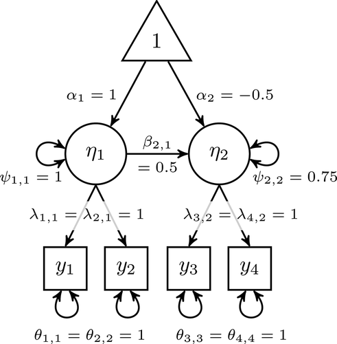
In this section, we illustrate how to obtain expected values of SEM parameters when treating ordinal data as continuous. We use the simple structural regression model depicted in as an example to work through five steps:
Figure 1. Path diagram depicting a 2-factor SEM with 4 normally distributed indicators. Any unstandardized population parameters not depicted in this diagram are fixed to zero.
1. We specify SEM population parameters and calculate the model-implied means and covariance matrix for using EquationEquation 5
(5)
(5) , represented by
and
.
2. We specify population thresholds that would discretize latent y variables.
3. We assign a numerical weight to each ordinal category, reflecting the numerical value of a discrete variable when treated as interval-level data.
4. We show how to analytically derive the expected means () and covariance matrix (
) implied by the specified thresholds and numerical weights. Furthermore, we show how to derive marginal third- and fourth-order moments (i.e., skew and kurtosis) of numerically weighted ordinal
variables.
5. We fit a SEM to and
that corresponds to the population model for LRVs, which provides population-level expected parameters (i.e., without sampling error) when treating
variables as continuous. Functions of those parameters analogously represent population-level expectations (e.g., model-based reliability coefficients, indirect effects).
We provideFootnote5 annotated R syntax and output to reproduce all steps in the file “Supp1-TechnicalDetails.pdf” on the Open Science Framework (OSF).
Step 1: Specify SEM for LRVs
Our population SEM has two factors (the first factor predicts the second factor), each with two indicators. Population values for all nonzero parameters are depicted in . Using EquationEquation 5(5)
(5) , the population means and covariance matrix are:
To verify these model parameters can be reproduced when fitting an appropriately specified model to and
, we used ML in lavaan with an arbitrary
. Using the configuration in with
and
as reference indicators, we fixed their loadings to 1 and intercepts to 0 for identification, freely estimating the loadings and intercepts of
and
. All factor and indicator (residual) variances were estimated, as well as factor means and the regression of
on
. Model fit was perfect,
, the unstandardized model parameters were identical to those in , and the standardized solution verified that the population slope
is already in a standardized metric because Var(
)
.
Step 2: Specify thresholds
For each variable we intend to discretize, we must next specify the thresholds in EquationEquation 7
(7)
(7) that would be used to discretize any sample data drawn from the population in EquationEquation 8
(8)
(8) . For the sake of illustration, we will discretize variables
–
into 3, 4, 5, and 6 categories, respectively. This requires
, 3, 4, and 5 thresholds, respectively.
Thresholds can be chosen directly using such criteria as (un)evenly spaced categories (e.g., Rhemtulla et al., Citation2012) or indirectly by first specifying probabilities per category that yield a desired marginal distribution of (i.e., the probability mass function of the categorical distribution; Li, Citation2016a, Citation2016b). We do the latter to illustrate the extra step of deriving thresholds from probability distributions. From an applied perspective, this might also be a more intuitive way to choose thresholds because one can easily imagine (or draw a picture of) a distribution of response categories. Categories that are more likely to elicit a response will have more weight (higher bars in a histogram) relative to other categories. The most difficult requirement would be that the probabilities of each category must sum to 1, but any arbitrary category weights can be transformed to probabilities by simply dividing by the sum of weights. For example, assigning weights of 5, 7, and 1 implies that the highest category is relatively rare, whereas the lowest category is only somewhat less likely than the middle; dividing by (
=) 13 yields probabilities of
,
, and
, respectively.
For indicators –
, we chose probabilities that yielded symmetric unimodal distributions that look approximately normal. The probabilities are displayed at the top of each category’s bar in . For
, we chose probabilities that yielded an asymmetric, positively skewed distribution whose mode was the lowest category, resembling a half-normal or Pareto distribution. Asymmetric thresholds can exacerbate attenuation of standardized factor loadings, in which case 7 rather than five categories is considered sufficient to treat as continuous (Rhemtulla et al., Citation2012).
Figure 2. Probability mass functions for ordinal variables. Corresponding normally distributed LRVs (
–
) have marginal means and variances implied by the population model in . Marginal probabilities are at the top of each bar, and upper thresholds are shown above each bar (except the lower threshold is shown above the highest category’s bar). Numerical weights assigned to each category are shown on the
-axis.
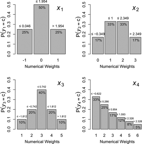
The thresholds between
categories are quantiles in a univariate normal distribution with the LRV’s
and
in EquationEquation 8
(8)
(8) . For example,
has
and
. To find the thresholds, one must first calculate the cumulative probabilities by summing the probabilities of all categories below each threshold. For example,
has
thresholds, with (left-tail) cumulative probabilities of 25% and (25% + 50% =) 75%, respectively. Likewise,
has
thresholds, with cumulative probabilities of 17%, (17% + 33% =) 50%, and (17% + 33% + 33% =) 83%, respectively.
Once cumulative probabilities below each threshold are calculated, the thresholds themselves can be found using almost any general statistical software package – for example,Footnote6 the qnorm() function in R. Above each bar in , that category’s upper threshold is displayed. The upper threshold of the highest category is , so instead displays the lower threshold (with inequality sign switched), which is redundant with the threshold displayed above the previous category’s bar.
It is important to note that the thresholds in are not the standardized thresholds () that would be estimated from observed contingency tables (i.e., Step 1 of least-squares estimation, before estimating polychoric correlations). Because the LRV distributions are latent (i.e., without a location or scale), they are arbitrarily assumed standard normal; thus, standardized thresholds are estimated, then used to estimate polychoric correlations (again, assuming all LRV variances = 1). There is no reason to struggle to specify SEM parameters that yield a standardized population
, but thresholds in could be transformed to
scores using the familiar formula:
If, however, only standard-normal quantiles were available (e.g., using tables that frequently appear in appendices of statistics textbooks), unstandardized thresholds could be derived by inverting EquationEquation 9(9)
(9) :
Step 3: Assign numerical weights to ordinal categories
Once thresholds have been chosen (or derived from chosen probabilities), no more population parameters would be needed to simulate ordinal data for a Monte Carlo study. However, to treat ordinal data as continuous, a numerical weight must be assigned to each category
. Weights for Likert scales are typically sequential integers beginning with 1, as we use for
and
in our example (see the
axes in ). However, some (e.g., binary) scales use 0 as the lowest category (as we use for
), and nothing prevents using negative numbers (as we use for
).
Equally spaced category weights reflect the (perhaps strong) assumption that the ordinal categories can be treated as interval-level data, which would be consistent with the choice to treat ordinal data as continuous. Depending on the content of an indicator’s scale description, unequal widths might also be justified. For example, Agresti (Citation2007, p. 42) provided an example of a discretized frequency outcome (average number of drinks per day), for which categories were labeled “0,” “<1,” “1–2,” “3–5,” and “”. Agresti (Citation2007) quite reasonably assigned
to “0” and assigned midpoints (i.e.,
,
, and
) of the ranges represented in the second, third, and fourth categories. The final category had no upper limit (so no midpoint), but
was assigned because very large latent frequencies were assumed rare.
Step 4: Calculate moments for numerically weighted ordinal variables
Sample means are calculated by summing scores, then dividing by the sample size , which is equivalent to summing the ratio of each score to
:
Because ordinal data consist of relatively few discrete values, we can multiply each value by the number of observations with that value, then divide that product by
where is the sample proportion (an estimate of category
’s probability) and
is the number of observations in category
. Populations are infinite, but what EquationEquation 11
(11)
(11) shows is that sample sizes are not needed to calculate the population mean of ordinal
variables because we specified the population probabilities
in Step 2.
The same principle applies to higher-order moments. The mean is the first raw moment of a distribution; the variance is the second central moment; and skewness and kurtosis are the third and fourth standardized central moments, respectively. Because the normal distribution has kurtosis = 3, excess kurtosis is frequently reported relative to 3. Univariate parameters for ordinal data with numerical weights are calculated as:
Note that must be calculated first because it is used to calculate higher-order central moments; likewise,
must be calculated second because it is used to standardize the third and fourth moments.
To illustrate, we show the calculations of the first two moments for , using numerical weights and probabilities for each category shown in :
so . All four univariate population moments in EquationEquation 12
(12)
(12) for each discretized LRV are shown in the left half of .
Table 1. Univariate and bivariate population moments for discretized latent response variables
Bivariate moments between ordinal variables
Covariance is a bivariate (mixed) central moment calculated similar to variance, but instead of summing the squared deviations of each category weight from the mean (weighted by marginal probabilities ), we sum the cross-products across all combinations of categories for a pair of variables (weighted by joint probabilities
). Adding a superscript to differentiate category weights
for
and
for
:
with indexing categories
of
and
indexing categories
of
.
Just as marginal probabilities of an ordinal variable are determined from the cumulative probabilities of its corresponding LRV distribution, joint probabilities of a pair of ordinal
variables are determined from cumulative probabilities of their bivariate LRV distribution. illustrates how the LRVs
and
are discretized into
and
categories, respectively, with their respective thresholds intersecting to form a two-way contingency table. The joint probabilities in each cell are calculated from bivariate-normal cumulative probabilities of each variable’s upper and lower thresholds (Olsson (Citation1979a), p. 447, Equationeq. 4)
(4)
(4) :
Figure 3. Contingency table of joint probabilities for
and
, with bivariate normal density of LRVs (
and
) depicted in the background (darker gray indicates higher probability density). Marginal probability distributions are depicted as smooth histograms on each axis, with marginal probabilities and numeric weight displayed between thresholds (dotted lines).
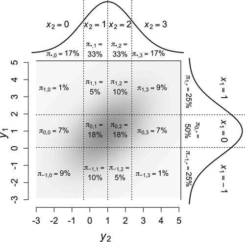
where is the bivariate-normal cumulative distribution function (CDF) with parameters
and
, up to thresholds
and
.
To illustrate, consider the probability in , whose upper thresholds demarcate the partition of the bivariate-normal distribution represented in the first righthand term of EquationEquation 15
(15)
(15) (i.e., all area below and to the left of that cell’s top-right corner). The second and third righthand terms in EquationEquation 15
(15)
(15) subtract cumulative probabilities below and to the left of (respectively) the same cell’s lower thresholds. Because the portion of bivariate density contained within cells
and
is subtracted twice, the cumulative probability is added back by the final righthand term in EquationEquation 15
(15)
(15) to compensate. The heat map underlying cells in shows that the highest-density portions of the bivariate-normal LRV distribution are contained within cells with greatest
. The right half of shows
(upper triangle) and the corresponding correlations (
) in the lower triangle, calculated using the assigned weights in , each
from EquationEquation 15
(15)
(15) , and each
from EquationEquation 12
(12)
(12) .
Bivariate moments between mixed variables
These methods can also be applied when the outcome is comprised of both continuous and discrete data. In this case, the population correlations () would comprise a mixture of polychoric, polyserial, and Pearson correlations. Given a discrete variable
, with weights
, thresholds
, and derived variance
, its polyserial correlation
with a continuous variable (i.e., on
’s LRV scale) can be converted to a point-polyserial correlation
(i.e., treating
’s ordinal scale as continuous; Olsson et al. (Citation1982), p. 340, Equationeq. 11)
(11)
(11) :
where is the normal (not cumulative) probability density function with parameters
and
. If consecutive integers are chosen for the weights, then EquationEquation 16
(16)
(16) simplifies because
reduces to 1 for all
, so the term can be dropped.
Although we do not focus on mixed variables for the remainder of the tutorial, we briefly illustrate how to obtain a population point-polyserial correlation. Suppose that we measured using a continuous response scale, but
was still measured with an ordinal 3-point scale. The polyserial correlation between
and LRV
is
(EquationEq. 8
(8)
(8) ), which we convert to a point-polyserial correlation using EquationEquation 16
(16)
(16) with the thresholds and weights for
in , ordinal-scale
in , and LRV distribution with
and
(EquationEq. 8)
(8)
(8) :
To convert to a polyserial covariance, simply multiply it by the SDs of
and
:
, which in this case is simply
. Our R syntax shows how to obtain an entire matrix among ordinal
and
indicators of the first factor but continuous
and
indicators of the second factor.
Step 5: Fit SEM to ordinal moments
Once and
have been obtained, one can fit any SEM using them as input data. Following our example at the end of Step 1, we fit an (otherwise) appropriately specified model using the same specifications, sample size, and estimator as when the model was fit to
and
. Because location and scale parameters depend on the arbitrary category weights chosen in Step 3, unstandardized results are not comparable. presents standardized solutions for covariance-structure parameters using
and
as input. Consistent with previous simulation results, expected standardized factor loadings for
were attenuated relative to
, more so for fewer categories. Although
had the most categories, the asymmetric thresholds led to greater attenuation than for
or
. In contrast, the structural parameter
was only negligibly attenuated (Li, Citation2016a, Citation2016b; Rhemtulla et al., Citation2012).
Table 2. Continuous-data SEM parameters and transformation bias
Illustrative analyses
In this section, we provide brief illustrations of how this method could potentially add value to analyses of real data. Subsequently, we illustrate the added value it can bring to simulation studies comparing estimators that rely on different assumptions about the discrete data.
Real-data application
Numerous simulation studies have investigated under what conditions ordinal data could provide unbiased estimates of standardized factor loadings and structural coefficients. Although there is strong agreement on certain conditions (e.g., binary outcomes should not be treated as continuous), delineations are less firm in others (e.g., 5–7 categories, depending on patterns of asymmetry in thresholds). For researchers whose data characteristics do not yield a clear choice, the method described here could assist in making a decision. By specifying hypothetical population parameters, researchers can calculate the expected differences in (standardized) parameters and assess whether the amount of transformation error would be tolerable.
To demonstrate, we utilized six indicators of emotional well-being from the 2012 Dutch sample () of Round 6 of the European Social Survey (ESS Round 6: European Social Survey, Citation2014). This is a subset of the data used by Jak and Jorgensen (Citation2017), which included data from multiple countries in addition to The Netherlands (also modeled by Huppert et al., Citation2009, to earlier ESS data). One case’s observations were missing for all six indicators, so only
observations were analyzed. Additional incomplete data were accommodated using full-information ML estimation (FIML) when data were treated as continuous or pairwise deletion when data were treated as ordinal.
Both estimators converged on proper solutions,Footnote7 and the first set of columns in compares the standardized factor loadings and factor correlation between estimators. Compared to using DWLS to rely on the LRV assumption, factor loadings are 5–15% lower when treating indicators as continuous with (robust) ML, whereas the factor correlation is only 2% lower under ML. These discrepancies could be attributed at least partly to transformation bias, which could already inform a researcher’s decision about whether to draw inferences given the LRV assumption. However, discrepancies might be smaller or larger in other samples drawn from the same population, so the researcher’s decision would depend on arbitrary differences between statistically comparable samples. Discrepancies could also be attributed at least partly to pairwise deletion making a more restrictive missing-completely-at-random assumption relative to FIML’s missing-at-random assumption (Lei & Shiverdecker, Citation2020). We can use the proposed methodFootnote8 to ascertain how much transformation bias could be expected irrespective of sampling error or the additional random process of missing data.
Table 3. CFA estimates discrepancies and transformation bias for ESS data
When the DWLS estimator converges on a solution (as in this case), a researcher could simply treat the polychoric correlations implied by those estimates as though they were the population correlation matrix, as well as assume that data would be discretized using the observed standardized thresholds. The second set of columns in show the expected transformation errors are similar to the observed discrepancies between estimators. This is not surprising and might indicate the limited value this method could add when deciding whether to treat discrete data as continuous. Future simulation research could be designed to reveal the degree to which expected transformation errors are more stable than discrepancies between different estimators of the same data.
However, it might not be ideal (or even possible) to use DWLS estimates as population parameters when calculating expected transformation errors. First, doing so would reify the estimated parameters, when the true parameters would certainly differ to varying degrees from sample estimates. Second, DWLS might not converge on a(n) (im)proper solution (e.g., in small samples), in which case a researcher might not even have the option of comparing DWLS and (robust) ML estimates. In the latter case, it could still be informative to demonstrate how much attenuation could be expected from ML relative to DWLS estimates with discrete indicators. Finally, even when DWLS converges, it could be more informative to explicitly choose different combinations of factor loadings and thresholds to serve as a sensitivity analysis of expected transformation error under different conditions. Such a sensitivity analysis might be particularly useful when researchers are considering the potential effects of collapsing categories (e.g., due to sparse data or because some categories are not used in one of multiple groups; DiStefano et al., Citation2021; Rutkowski et al., Citation2019).
In our ESS example, we specified moderate-to-high standardized loadings (0.6–0.8) within each factor, and we crossed this with moderate (for Factor 1’s indicators) and extreme asymmetry of thresholds (for Factor 2’s indicators); we specified moderate asymmetry and cross-loadings of 0.35 for the multidimensional indicator. The final set of columns in reveal that analyzing discretized data as continuous could yield both higher and lower (standardized) factor loadings when asymmetry is moderate, whereas extreme asymmetry yields only lower loadings. More substantial expected transformation error was generally associated with greater asymmetry and lower loadings. If a researcher could not obtain DWLS results for their data, they could provide (robust) ML results and use this information to explain how the DWLS results could be expected to differ if available. Furthermore, simulations have shown the same conditions that yield substantial transformation error can lead to other types of problems (e.g., low coverage rates for parameters and inflated Type I errors for model fit; Rhemtulla et al., Citation2012), so this information could inform researchers whether to interpret (robust) ML results conservatively in the absence of DWLS for comparison.
Monte Carlo simulation study
To demonstrate the added value this method could bring to simulation studies, we replicated one condition from Rhemtulla et al. (Citation2012), who compared robust ML to unweighted least-squares for categorical indicators, which is equivalent to DWLS but replaces the diagonal weight matrix with an identity matrix. We chose one of the conditions that yielded large discrepancies between robust ML and ULS results. The population model was a two-factor CFA with five normally distributed latent-response indicators per factor. For each factor, the standardized loadings ranged from 0.3 to 0.7 in increments of 0.1, the factor correlation was 0.3, and two extremely asymmetric thresholds (,
) discretized each LRV into three categories. We simulated 1000 samples of
, which was also the sample size used when fitting the continuous-data CFA to the expected moments of the discretized population. R syntax and output for all analyses in this section are provided on the OSF (https://osf.io/s8tdhlink) in the file “Supp3-replicateRhemtulla2012.pdf.”
Rhemtulla et al. (Citation2012, , ) reported the empirical skew and kurtosis in each of 60 data-generating conditions, estimated using an asymptotically large sample of = 1,000,000 observations to minimize sampling error. The first advantage of the method proposed here is that it yields expected skew and kurtosis without measurement error, and that it can do so more quickly. Using R (version 4.1.0 R Core Team, Citation2021) on a Macintosh laptop with a 2.6 GHz Intel Core i7 processor, simulating the large sample in our one condition and calculating skew and kurtosis took 1.896 s of elapsed time, whereas deriving error-free skew and kurtosis from the population moments took only 0.063 s of elapsed time. One could extrapolate that for all 60 conditions, the analytical approach presented here would require <4 s to obtain (without sampling error) what would require almost 2 min by simulating large samples – admittedly, a minor advantage.
Using the analytically derived moments of discretized data, shows the expected transformation error (asterisks, free of sampling error) closely matches the “bias” reported by Rhemtulla et al. (Citation2012, see first column of the table on p. 4 of their online supplement) for this condition, depicted as horizontal line segments. Thus, a computationally intensive simulation might not be necessary for researchers solely interested in investigating transformation error (attenuation due to discretization). However, researchers are typically interested in more than accuracy of point estimates, such as uncertainty (e.g., CI coverage, bias), model fit (e.g., Type I error rates for test statistics), or missing-data methods (e.g., deletion and imputation methods, two-stage or full-information estimators). When such methods require Monte Carlo simulation to estimate frequency properties, the analytical approach can still have value insofar as decomposing transformation error from estimation bias (EquationEq. 1)
(1)
(1) .
Figure 4. Monte Carlo results replicating one condition from Rhemtulla et al. (Citation2012).
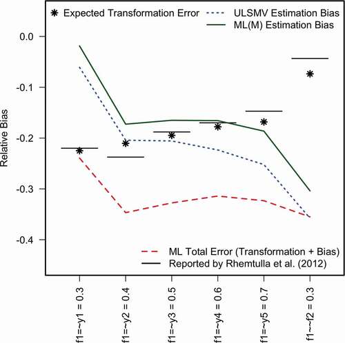
Our rates of nonconvergence and Heywood cases using lavaan differ from Rhemtulla et al. (Citation2012, reported in the top tables on pages 2 and 3 of their online supplement), who used Mplus. But given convergence on a proper solution in >80% of samples, our replication is sufficient for the purposes of illustration. We calculated the total bias–comparable to the bias reported by Rhemtulla et al. (Citation2012),–under (robust) ML and (categorical) ULS, but we calculated relative bias by dividing the difference by the population parameter (i.e., a percentage). Additionally, we calculated relative bias of ML estimates in terms of transformation error (i.e., using the expected parameters in the discrete scale rather than the LRV scale as a reference). shows the total relative bias of ML estimates (red dashed line) are generally much lower than the population expectations or the analogous quantities derived from what Rhemtulla et al. (Citation2012) reported. Most disturbing is that the factor correlation estimates were much more underestimated than expected. ML(M) and ULS(MV) estimation bias was also substantially more negative than expected. Despite not being asymptotically large enough to yield consistent estimates, the discrepancies from population expectations might motivate a researcher to investigate whether something unexpected went wrong with the simulation–another added value of using the proposed method–but that goes beyond the scope of mere illustration.
Discussion
Our tutorial demonstrated how to derive the uni- and bivariate moments of numerically weighted discrete data, given their thresholds and LRV covariance matrix. We also demonstrated that fitting a hypothesized SEM to these analytically derived moments is a simple numerical procedure for obtaining expected values of parameters that would result from an analysis treating the data as continuous. This straightforward process works for models that include both measurement and structural components, as well as combinations of discrete and continuous data. Consistent with previous Monte Carlo studies (Li, Citation2016a, Citation2016b; Rhemtulla et al., Citation2012), our applications demonstrated that both fewer categories and asymmetric thresholds resulted in greater attenuation of measurement model parameters, yet negligible bias of structural parameters.
However, the procedure we described assumes bivariate normality of LRVs, given the use of a multivariate-normal CDF. In contrast to a probit link, a logit link is quite popular for its real-world interpretability through transformation to an odds ratio, but would assume LRVs follow a logistic distribution (Agresti, Citation2007), whose current implementations unfortunately carry restrictive limitations on the size and distribution of correlation and scale parameters (Kotz et al., Citation2000). A promising alternative is the student-t approximation (Hahn & Soyer, Citation2005), but further evaluation is needed to assess its suitability in this context. Additionally, our numerical procedure provides only expected parameter values, but evaluating SEs and model fit statistics is often of equal interest. However, the conditions which lead to greater parameter bias (smaller and
, greater asymmetry of thresholds, LRVs deviate greater from normality) are those that lead to greater SE bias and inflation of Type I errors for fit statistics (Rhemtulla et al., Citation2012). So investigating discrepancies as in could still be useful for researchers deciding whether to treat data there as continuous or discrete.
Disclosure statement
No potential conflict of interest was reported by the author(s).
Additional information
Funding
Notes
1 It could be argued that this is not “bias” at all (Robitzsch, Citation2020).
2 An exception is W. Wu et al. (Citation2015), who assessed bias with regard to a scale composite, whose location and scale are determined by the observed response scale.
3 In the special case that both variables are binary, this is called the tetrachoric correlation.
4 In the special case of a binary variable, this is called the biserial correlation.
5 OSF project located at https://osf.io/s8tdh.
6 Other examples include NORM.INV in Excel, IDF.NORMAL in SPSS, and QUANTILE in SAS.
7 R syntax and output for all analyses in this section are provided on the OSF (https://osf.io/s8tdhlink) in the file “Supp2-RealDataExample.pdf”.
8 The method is implemented in the function lrv2ord(), part of the R package semTools (Jorgensen et al., Citation2020).
References
- Agresti, A. (2007). An introduction to categorical data analysis (2nd ed.). Hoboken NJ.
- Agresti, A. (2010). Analysis of ordinal categorical data. Wiley.
- Bandalos, D. L. (2014). Relative performance of categorical diagonally weighted least squares and robust maximum likelihood estimation. Structural Equation Modeling, 21, 102–116. https://doi.org/https://doi.org/10.1080/10705511.2014.859510
- Barendse, M., Oort, F., & Timmerman, M. (2015). Using exploratory factor analysis to determine the dimensionality of discrete responses. Structural Equation Modeling, 22, 87–101. https://doi.org/https://doi.org/10.1080/10705511.2014.934850
- Chalmers, R. P. (2018). On misconceptions and the limited usefulness of ordinal alpha. Educational and Psychological Measurement, 78, 1056–1071. https://doi.org/https://doi.org/10.1177/0013164417727036
- Chen, P.-Y., Wu, W., Garnier-Villarreal, M., Kite, B. A., & Jia, F. (2020). Testing measurement invariance with ordinal missing data: A comparison of estimators and missing data techniques. Multivariate Behavioral Research, 55, 87–101. https://doi.org/https://doi.org/10.1080/00273171.2019.1608799
- DiStefano, C., Shi, D., & Morgan, G. B. (2021). Collapsing categories is often more advantageous than modeling sparse data: Investigations in the CFA framework. Structural Equation Modeling, 28, 237–249. https://doi.org/https://doi.org/10.1080/10705511.2020.1803073
- DiStefano, C. (2002). The impact of categorization with confirmatory factor analysis. Structural Equation Modeling, 9, 327–346. https://doi.org/https://doi.org/10.1207/S15328007SEM0903_2
- ESS Round 6: European Social Survey. (2014). ESS-6 2012 documentation report (2.1 ed.; Tech. Rep.). Bergen, Norway. https://www.europeansocialsurvey.org/data/download.html?r=6
- Foldnes, N., & Grønneberg, S. (2020). Pernicious polychorics: The impact and detection of underlying non-normality. Structural Equation Modeling, 27, 525–543. https://doi.org/https://doi.org/10.1080/10705511.2019.1673168
- Green, S. B., & Yang, Y. (2009). Reliability of summed item scores using structural equation modeling: An alternative to coefficient alpha. Psychometrika, 74, 155–167. https://doi.org/https://doi.org/10.1007/s11336-008-9099-3
- Hahn, E. D., & Soyer, R. (2005). Probit and logit models: Differences in the multivariate realm.
- Huppert, F. A., Marks, N., Clark, A., Siegrist, J., Stutzer, A., Vittersø, J., & Wahrendorf, M. (2009). Measuring well-being across Europe: Description of the ESS well-being module and preliminary findings. Social Indicators Research, 91, 301–315. https://doi.org/https://doi.org/10.1007/s11205-008-9346-0
- Jak, S., & Jorgensen, T. D. (2017). Relating measurement invariance, cross-level invariance, and multilevel reliability. Frontiers in Psychology, 8(1640). https://doi.org/https://doi.org/10.3389/fpsyg.2017.01640
- Jia, F., & Wu, W. (2019). Evaluating methods for handling missing ordinal data in structural equation modeling. Behavior Research Methods, 51, 2337–2355. https://doi.org/https://doi.org/10.3758/s13428-018-1187-4
- Jöreskog, K. G. (1990). New developments in LISREL: Analysis of ordinal variables using polychoric correlations and weighted least squares. Quality and Quantity, 24, 387–404. https://doi.org/https://doi.org/10.1007/BF00152012
- Jorgensen, T. D., Pornprasertmanit, S., Schoemann, A. M., & Rosseel, Y. (2020). semTools: Useful tools for structural equation modeling [Computer software manual]. https://cran.r-project.org/package=semTools (R package version 0.5-3)
- Kotz, S., Balakrishnan, N., & Johnson, N. L. (2000). Multivariate logistic distributions. In Continuous multivariate distributions, volume 1: Models and applications (pp. 551–576). Wiley.
- Lei, P.-W., & Shiverdecker, L. K. (2020). Performance of estimators for confirmatory factor analysis of ordinal variables with missing data. Structural Equation Modeling, 27, 584–601. https://doi.org/https://doi.org/10.1080/10705511.2019.1680292
- Li, C.-H. (2016a). Confirmatory factor analysis with ordinal data: Comparing robust maximum likelihood and diagonally weighted least squares. Behavior Research Methods, 48, 936–949. https://doi.org/https://doi.org/10.3758/s13428-015-0619-7
- Li, C.-H. (2016b). The performance of ml, dwls, and uls estimation with robust corrections in structural equation models with ordinal variables. Psychological Methods, 21, 369–387. https://doi.org/https://doi.org/10.1037/met0000093
- Liu, Y., & Thompson, M. S. (2020). General factor mean difference estimation in bifactor models with ordinal data Structural Equation Modeling, 28, 423–439. https://doi.org/https://doi.org/10.1080/10705511.2020.1833732
- Maydeu-Olivares, A., Coffman, D. L., & Hartmann, W. M. (2007). Asymptotically distribution-free (ADF) interval estimation of coefficient alpha. Psychological Methods, 12, 157–176. https://doi.org/https://doi.org/10.1037/1082-989X.12.2.157
- McArdle, J. J., & McDonald, R. P. (1984). Some algebraic properties of the reticular action model for moment structures. British Journal of Mathematical and Statistical Psychology, 37, 234–251. https://doi.org/https://doi.org/10.1111/j.2044-8317.1984.tb00802.x
- Meade, A. W., Johnson, E. C., & Braddy, P. W. (2008). Power and sensitivity of alternative fit indices in tests of measurement invariance. Journal of Applied Psychology, 93, 568–592. https://doi.org/https://doi.org/10.1037/0021-9010.93.3.568
- Muthén, B. O., & Asparouhov, T. (2002). Latent variable analysis with categorical outcomes: Multiple-group and growth modeling in M plus (Tech. Rep.). (Mplus web note 4). http://www.statmodel.com/
- Muthén, B. O. (1984). A general structural equation model with dichotomous, ordered categorical, and continuous latent variable indicators. Psychometrika, 49, 115–132. https://doi.org/https://doi.org/10.1007/BF02294210
- Muthén, L. K., & Muthén, B. O. (1998–2017). Mplus user’s guide (8th ed.). [Computer software manual]. Muthén & Muthén.
- Olsson, U., Drasgow, F., & Dorans, N. J. (1982). The polyserial correlation coefficient. Psychometrika, 47, 337–347. https://doi.org/https://doi.org/10.1007/BF02294164
- Olsson, U. (1979a). Maximum likelihood estimation of the polychoric correlation coefficient. Psychometrika, 44, 443–460. https://doi.org/https://doi.org/10.1007/BF02296207
- Olsson, U. (1979b). On the robustness of factor analysis against crude classification of the observations. Multivariate Behavioral Research, 14, 485–500. https://doi.org/https://doi.org/10.1207/s15327906mbr1404_7
- R Core Team. (2021). R: A language and environment for statistical computing [Computer software manual]. Vienna, Austria. https://www.R-project.org/
- Raykov, T., & Marcoulides, G. A. (2015). On examining the underlying normal variable assumption in latent variable models with categorical indicators. Structural Equation Modeling, 22, 581–587. https://doi.org/https://doi.org/10.1080/10705511.2014.937846
- Rhemtulla, M., Brosseau-Liard, P. É., & Savalei, V. (2012). When can categorical variables be treated as continuous? A comparison of robust continuous and categorical SEM estimation methods under suboptimal conditions. Psychological Methods, 17, 354–373. https://doi.org/https://doi.org/10.1037/a0029315
- Robitzsch, A. (2020). Why ordinal variables can (almost) always be treated as continuous variables: Clarifying assumptions of robust continuous and ordinal factor analysis estimation methods. Frontiers in Education, 5, 177. https://doi.org/https://doi.org/10.3389/feduc.2020.589965
- Rosseel, Y. (2012). lavaan: An R package for structural equation modeling and more. Journal of Statistical Software, 48, 1–36. https://doi.org/https://doi.org/10.18637/jss.v048.i02
- Rutkowski, L., Svetina, D., & Liaw, Y.-L. (2019). Collapsing categorical variables and measurement invariance. Structural Equation Modeling, 26, 790–802. https://doi.org/https://doi.org/10.1080/10705511.2018.1547640
- Sass, D. A., Schmitt, T. A., & Marsh, H. W. (2014). Evaluating model fit with ordered categorical data within a measurement invariance framework: A comparison of estimators. Structural Equation Modeling, 21, 167–180. https://doi.org/https://doi.org/10.1080/10705511.2014.882658
- Satorra, A., & Saris, W. E. (1985). Power of the likelihood ratio test in covariance structure analysis. Psychometrika, 50, 83–90. https://doi.org/https://doi.org/10.1007/BF02294150
- Savalei, V. (2014). Understanding robust corrections in structural equation modeling. Structural Equation Modeling, 21, 149–160. https://doi.org/https://doi.org/10.1080/10705511.2013.824793
- Stark, S., Chernyshenko, O. S., & Drasgow, F. (2006). Detecting differential item functioning with confirmatory factor analysis and item response theory: Toward a unified strategy. Journal of Applied Psychology, 91, 1292–1306. https://doi.org/https://doi.org/10.1037/0021-9010.91.6.1292
- Vispoel, W. P., Morris, C. A., & Kilinc, M. (2019). Using generalizability theory with continuous latent response variables. Psychological Methods, 24, 153–178. https://doi.org/https://doi.org/10.1037/met0000177
- Wirth, R., & Edwards, M. C. (2007). Item factor analysis: Current approaches and future directions. Psychological Methods, 12, 58–79. https://doi.org/https://doi.org/10.1037/1082-989X.12.1.58
- Wu, H., & Estabrook, R. (2016). Identification of confirmatory factor analysis models of different levels of invariance for ordered categorical outcomes. Psychometrika, 81, 1014–1045. https://doi.org/https://doi.org/10.1007/s11336-016-9506-0
- Wu, W., Jia, F., & Enders, C. K. (2015). A comparison of imputation strategies for ordinal missing data on Likert scale variables. Multivariate Behavioral Research, 50, 484–503. https://doi.org/https://doi.org/10.1080/00273171.2015.1022644
- Zumbo, B. D., Gadermann, A. M., & Zeisser, C. (2007). Ordinal versions of coefficients alpha and theta for Likert rating scales. Journal of Modern Applied Statistical Methods, 6, 21–29. https://doi.org/https://doi.org/10.22237/jmasm/1177992180