The Challenge of Generating Causal Hypotheses Using Network Models

Abstract

Statistical network models based on Pairwise Markov Random Fields (PMRFs) are popular tools for analyzing multivariate psychological data, in large part due to their perceived role in generating insights into causal relationships: a practice known as causal discovery in the causal modeling literature. However, since network models are not presented as causal discovery tools, the role they play in generating causal insights is poorly understood among empirical researchers. In this paper, we provide a treatment of how PMRFs such as the Gaussian Graphical Model (GGM) work as causal discovery tools, using Directed Acyclic Graphs (DAGs) and Structural Equation Models (SEMs) as causal models. We describe the key assumptions needed for causal discovery and show the equivalence class of causal models that networks identify from data. We clarify four common misconceptions found in the empirical literature relating to networks as causal skeletons; chains of relationships; collider bias; and cyclic causal models.

Keywords:

• Causal hypotheses
• conditional dependence
• directed acyclic graph (DAG)
• Gaussian graphical model
• network approach
• statistical equivalence

1. Introduction

The network approach to psychopathology is a theoretical framework in which mental disorders are viewed as arising from direct causal interactions between symptoms (Borsboom, 2017; Borsboom & Cramer, 2013). This theoretical viewpoint, along with accompanying methodological developments, has in turn spurred a rapid increase in the number of empirical papers which fit statistical network models based on Pairwise Markov Fields (PMRFs) to cross-sectional data (Epskamp, Waldorp, et al., 2018; Haslbeck & Waldorp, 2020; Van Borkulo et al., 2014). A recent review paper found 141 such papers between 2008 and 2018 alone, with the rate of publication increasing rapidly between 2016 and 2018 (Robinaugh et al., 2020). The most popular of these statistical network models, the Gaussian Graphical Model (GGM), yields an undirected network in which the connections between variables represent partial correlations, that is, estimates of the conditional dependency between each pair of variables when controlling for all other variables in the network.

Network methodologists have frequently suggested that these models can be used to generate causal hypotheses about the underlying causal system (Borsboom & Cramer, 2013; Epskamp, van Borkulo, et al., 2018; Epskamp, Waldorp, et al., 2018; Robinaugh et al., 2020): The absence of a connection is interpreted as reflecting the absence of a directed causal relationship, although the presence of a network connection may not reflect the presence of a causal relationship. In practice, this means that network parameters estimated from empirical data are often interpreted as reflecting causal relationships. As such, one could reasonably characterize much of empirical network analysis as a form of causal discovery, a term from the causal modeling literature which describes the process of using statistical relationships, like conditional dependencies, to make inferences about the structure and nature of directed causal relationships (Eberhardt, 2017; Glymour et al., 2019; Pearl, 2009; Peters et al., 2017; Spirtes et al., 2000).

Despite the parallels between psychological network analysis and causal discovery, the literature so far lacks a clear description of how these two practices relate, and as such, how well statistical network models work as causal discovery tools. A lack of clarity around these issues has led to several misconceptions among applied researchers. For example, statistical networks are often erroneously interpreted as causal skeletons, identifying the presence but not the direction of causal links between variables (e.g., Boschloo et al., 2016; Haslbeck & Waldorp, 2018; van Borkulo et al., 2015). Even methodological papers which accurately characterize the relationship between statistical networks and directed causal models (Borsboom & Cramer, 2013; Epskamp, van Borkulo, et al., 2018; Epskamp, Waldorp, et al., 2018) typically do not outline the key assumptions which are needed for causal discovery to work in practice, the type of causal structure(s) about which inferences are to be made, or what other types of inferences, for instance regarding the sign or size of causal effects, are or are not licensed by estimated network models.

In this tutorial paper, we aim to clarify how statistical network models work as causal discovery tools, outlining the challenges and opportunities which come along with this and addressing common misconceptions which are present in the psychological network literature. To this end, we first review the basics of statistical network models and how they relate to Directed Acyclic Graphs (DAGs), a common way to represent directed causal relationships that are related to linear structural equation models (SEMs) familiar to social science researchers (Bollen & Pearl, 2013; Pearl, 2009, 2013). Following this, we describe how statistical network models could be used as causal discovery tools, with an emphasis on clarifying the assumptions we need for “causal hypothesis generation” to work in practice. We show that different network models allow researchers to identify so-called equivalence classes of causal structure, a concept we introduce to the statistical network literature and which allows us to understand exactly which inferences can and cannot be made from network model parameters. In the third part of the paper, we clarify several misconceptions in the empirical literature regarding the causal interpretation of network models, including the role of common effect variables, the positive manifold, and the relationship between statistical network models and cyclic causal models. We end with a brief discussion of alternative methods for causal discovery, and alternative ways of using network models to test the implications of a causal model.

2. Background

In this section, we will give a brief overview of two different types of graphical models: The Pairwise Markov Random Field (PMRF), which is the basis of statistical network modeling, and the Directed Acyclic Graph (DAG), which is commonly used in the causal inference literature. We also review two commonly used statistical models associated with each: the Gaussian Graphical Model (GGM) and the linear Structural Equation Model (SEM).

2.1. The Pairwise Markov Random Field and Gaussian Graphical Model

The PMRF is a graphical model that consists of variables (nodes) and undirected connections (edges) between those variables. Edges are either present or absent, but do not have a particular value (weight) associated with them. The presence of an edge denotes a particular form of conditional dependence between variables: an edge between a variable X_i and another variable X_j is present if and only if those variables are dependent (i.e. are statistically associated) when we condition on the set of all other variables in the network (denoted with ${\mathit{X}}_{-(i,j)}$). In this context, conditioning on these variables means that we control for them statistically, that is, that we obtain the association between X_i and X_j given the value of the other variables in the network. The absence of an edge in a PMRF in turn denotes that X_i and X_j are independent, that is, not statistically associated, conditional on all other variables. We denote this as (1) $$X_i\hspace{0.17em}\perp \perp \hspace{0.17em}{X}_j\hspace{0.17em}|\hspace{0.17em}{\mathit{X}}_{-(i,j)},$$(1) where $\perp \perp$ stands for independence between a pair of random variables and $\cancel{\perp \perp }$ stands for dependence (Dawid, 1979; Lauritzen, 1996).

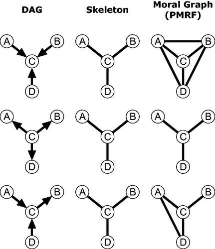
In Figure 1a we show an example of a PMRF made up of four variables relating to burnout: levels of social support (Support), work pressure (Pressure), Stress, and Worry. From this graph, we can read off the aforementioned conditional dependency relationships among those four variables. Support, Pressure, and Stress are all connected to one another by undirected edges indicating, for instance, that Pressure and Support are dependent conditional on Stress and Worry (Pressure $\cancel{\perp \perp }$ Support $|$ Stress, Worry). Worry, however, is only connected to Stress: This means that Worry is dependent on Stress when we condition on Pressure and Support (Worry $\cancel{\perp \perp }$ Stress $|$ Pressure, Support), but that Worry is independent of Pressure and Support conditional on Stress (Worry $\perp \perp$ Pressure $|$ Stress, Support and Worry $\perp \perp$ Support $|$ Stress, Pressure).

Figure 1. Four different types of network (graphical model), all describing different characteristics of the same system. Panel (a) depicts the Pairwise Markov Random Field (PMRF), panel (b) Gaussian Graphical Model (GGM), (c) Directed Acyclic Graph (DAG) and (d) a linear Structural Equation Model (SEM). In the weighted graphs, red edges depict negative relationships, blue edges depict positive edges, and the width of the edge is determined by the absolute value of the relationship (partial correlations for the GGM and regression weights for the SEM).

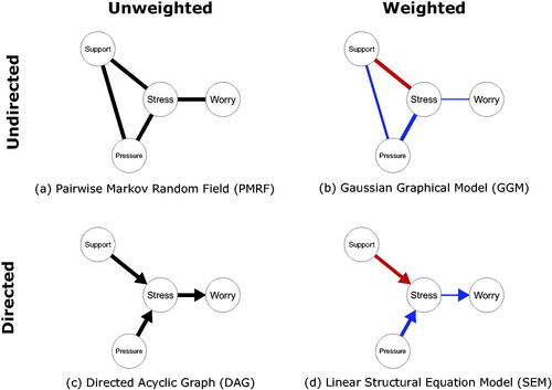
Statistical network models, such as the Gaussian Graphical Model (GGM) and Ising model are particular instances of PMRF models, which use assumptions about the distributions of the variables, and their relationships with one another, to produce a PMRF with weighted edges (Epskamp, Waldorp, et al., 2018; Van Borkulo et al., 2014). In the current paper we will focus on the GGM, a popular network model for variables that follow a Gaussian (i.e. normal) distribution $\mathit{X}\sim \mathcal{N}(\mathit{\mu },\mathbf{\Sigma })$ (Cox & Wermuth, 1996; Dempster, 1972; Epskamp, Waldorp, et al., 2018; Lauritzen, 1996). The conditional dependency relationships depicted by the weighted edges in a GGM are based on partial correlations: In the network visualization, stronger partial correlations are represented by thicker edges. A partial correlation can be interpreted in a similar way to multiple linear regression coefficients. Imagine we perform a regression analysis with X_i as the outcome variable, and X_j and all other variables ${\mathit{X}}_{-(i,j)}$ as predictors. The regression coefficient for X_j is an example of an estimate of a conditional relationship between X_i and X_j controlling for all other predictor variables. A partial correlation can be interpreted similarly, except that partial correlations are undirected, that is, no distinction is made between X_i and X_j as an outcome or predictor variable. An example of a GGM is shown in Figure 1b. The positive edge connecting Stress and Worry indicates that keeping both Support and Pressure constant, high scores for Stress tend to co-occur with high scores for Worry, with the size of the edge denoting the strength of that relationship. Here again, the absence of an edge is taken to denote that variables are conditionally independent (i.e. have a zero partial correlation) controlling for all other variables in the network.

2.2. Directed Acyclic Graphs and Linear SEMs

A Directed Acyclic Graph (DAG) is a graphical model consisting of unweighted directed edges between variables, with “acyclic” referring to the property that no cycles or feedback loops (e.g. $X_i\hspace{0.17em}\leftrightarrows \hspace{0.17em}{X}_j$) are permitted between variables. DAGs (also known as Bayesian Networks) are commonly used to represent causal relationships between variables, where the directed edge $X_i\to X_j$ denotes that an intervention to change the value of X_i will lead to a change in the probability distribution of X_j (for an accessible, more elaborate introduction to the use of DAGs in causal inference see, amongst others Hernan & Robins, 2010; Pearl et al., 2016; Rohrer, 2018). The DAG structure is often described in “familial” terms: Directed edges $X_i\to X_j$ connect parent nodes or causes (X_i) to children nodes or effects (X_j). Nodes that share a common child, but are not directly connected to one another, are termed unmarried parents, while children, as well as children of children (and so forth), are called descendants. An example of a DAG is shown in Figure 1c, where Support and Pressure are unmarried parents of Stress, Stress is a parent of Worry, and we can say that Worry is a descendant of Support, Pressure, and Stress.

As well as representing causal structure, the DAG describes which variables in the graph are conditionally dependent and independent from one another, but does so in a different and more detailed manner than the PMRF. Specifically, a DAG describes the conditional dependencies present in a set of random variables X according to the so-called local Markov condition (Spirtes et al., 2000), which states that each variable X_i is conditionally independent of its non-descendants, given its parents: (2) $$X_i\hspace{0.17em}\perp \perp \hspace{0.17em}{\mathit{X}}_{-de(i)}\hspace{0.17em}|\hspace{0.17em}{\mathit{X}}_{pa(i)}.$$(2)

This condition can be used to read off several different conditional (in)dependence relations between pairs of variables in the DAG. For example, in Figure 1c, we can derive that Support and Pressure are marginally independent, that is, independent when not conditioning on any other variables (Support $\perp \perp$ Pressure $|\varnothing$), because Pressure is not a descendant of Support, and Support has no parents in this graph ($pa($Support$)$ $=\varnothing$).

Further conditional (in)dependence relationships between any pair of variables can be derived from the graph using d-separation rules, which follow the local Markov condition (Pearl, 2009). The most important of these rules for the current paper relates to situations in which two variables share a common effect, also known as a collider structure $X_i\to X_k\leftarrow X_j.$ From d-separation rules, we know that in a DAG, parent variables X_i and X_j are dependent conditional on their common child X_k. In Figure 1c, although Support and Pressure are marginally independent, they are dependent when conditioning on Stress (Support $\cancel{\perp \perp }$ Pressure $|$ Stress). This implies that if, for example, we were to statistically control for levels of Stress, we would expect to see a non-zero statistical dependency between Support and Pressure. On the other hand, if we do not control for Stress, we would expect to see no such statistical dependency between Support and Pressure.

While the DAG describes which variables are causally dependent on one another, and we can use the accompanying d-separation rules to derive which statistical dependencies are implied by these causal relationships, the DAG itself does not specify any particular model for these relationships. That is, it does not tell us what the functional form of those causal relationships is (e.g., linear or non-linear), nor does it represent any distributional assumptions about the variables involved (e.g., Gaussian or something else). If we want to specify a weighted version of a DAG, we need to introduce assumptions about the form of the causal model which the DAG represents (referred to as a structural causal model in the causal inference literature; Pearl, 2009). If we assume that the causal relationships between variables are linear, and the distribution of the noise terms (i.e. residuals) are Gaussian, then we can represent the causal system as a Structural Equation Model (Bollen, 1989).¹ Such a model is essentially a multivariate regression where child nodes are predicted by their parents: (3) $$\mathit{X}=\mathit{\alpha }+\mathit{BX}+\mathit{ϵ}$$(3) where B is a p × p matrix that contains the regression coefficients, $\mathit{\alpha }$ represents a $p\times 1$ vector that contains the intercepts, and $\mathit{ϵ}$ represents a $p\times 1$ vector of uncorrelated noise terms, following a Gaussian distribution with mean zero and a diagonal variance-covariance matrix $\mathbf{\Psi }.$ The regression coefficients B can be used to create a graphical representation of the SEM model as a weighted DAG, where the size of the regression coefficients determines the thickness of the directed edges in the graph, and the sign of the coefficient determines their color, as shown in Figure 1d. In this example, Support has a negative causal effect on Stress (depicted in red), while Pressure has a positive effect on Stress, and Stress has a weaker positive effect on Worry (both depicted in blue).

In the remainder of the paper, we will consider the situation in which researchers wish to use statistical network models to make inferences about directed causal relationships, as represented by a DAG. The relationship between PMRFs and DAGs as graphical models, and in turn the relationship between GGMs and SEMs as statistical models, informs us about the advantages, disadvantages, and key considerations of such an approach.

3. Network Models as Causal Discovery Tools

Many researchers use the patterns of conditional (in)dependence in statistical network models to make inferences about the underlying causal relationships between those variables, a practice referred to as generating causal hypotheses (Borsboom & Cramer, 2013; Epskamp, van Borkulo, et al., 2018; Epskamp, Waldorp, et al., 2018). In the causal modeling literature, using estimated statistical (in)dependencies to infer the structure of causal relationships between variables is known as causal discovery (Eberhardt, 2017; Glymour et al., 2019; Pearl, 2009; Peters et al., 2017; Spirtes et al., 2000). In general, causal discovery from observational data is challenging, in part because the causal structure is typically not uniquely identified (Glymour et al., 2019; Scheines et al., 1998). Even if we assume, for example, that the causal structure is a linear SEM model, we know that there will typically be many different statistically equivalent SEM models which produce the same patterns of statistical dependencies in observational data (Bollen, 1989). This means that rather than being able to recover the causal graph, we can instead typically only identify a set of statistically equivalent but causally-distinct models.

In the following, we present an analysis of statistical network models as causal discovery tools. Although it is evident that this is how network models are often used in practice, network models are rarely if ever explicitly presented as methods for causal discovery. As a consequence, while the issues involved in causal discovery are already well-understood in the causal modeling literature, the relevance of these issues to empirical researchers using statistical network models has yet to be made clear. To address this problem, we discuss the advantages and disadvantages of using PMRFs and GGMs as causal discovery tools. We show how these models can in principle identify some aspects of causal structure but fall short in identifying others and describe under what conditions this kind of causal discovery is possible. We begin in the simplest and most ideal setting, describing how and when the population level PMRF could be used for causal discovery, then evaluating what information is gained by using the weighted GGM, before discussing the difficulties which arise when working with estimated network models.

3.1. Causal Discovery with PMRFs

To define how network models operate as causal discovery tools, we can make use of the known relationship between the structure of a DAG and the structure of a PMRF (Lauritzen, 1996; Spirtes et al., 2000). When the underlying causal structure is a DAG, then the corresponding PMRF can be viewed as the moral graph of that DAG. The moral graph is an undirected graph obtained by; first “marrying” all “unmarried parents” in the DAG, that is, drawing an undirected edge between all nodes that share a descendant but are not already connected by an edge; and second, by then replacing all directed edges with undirected edges. The moral graph, therefore, contains an undirected edge if either (a) these two nodes are connected by a directed edge in the DAG or (b) these two nodes are involved in a collider structure (Lauritzen, 1996; Spirtes et al., 2000; Wermuth & Lauritzen, 1983).² For example, comparing Figures 1a and c, the PMRF (a) contains an undirected version of all of the edges in the DAG (c), in addition to an edge connecting the unmarried parent's Support and Pressure, just as expected from the definition of the moral graph.

This relationship between PMRF and DAG structure means that two heuristics can be defined which describe what inferences can be made—under ideal conditions—about the presence or absence of a causal relationship between two variables based on the presence or absence of an edge between those same variables in the network. These two heuristics are described by network methodologists as the rules which researchers can use to “generate causal hypotheses” from an estimated network model (Borsboom & Cramer, 2013; Epskamp, van Borkulo, et al., 2018; Epskamp, Waldorp, et al., 2018):

Heuristic 1: An edge between two variables in the PMRF ($X_i-X_j$) indicates that two variables share either a direct causal link ($X_i\to X_j$ or $X_i\leftarrow X_j$) or a common effect ($X_i\to X_k\leftarrow X_j$)

Heuristic 2: The absence of an edge between two variables ($X_i-/X_j$) indicates that these two variables do not share a direct causal link ($X_i\nrightarrow X_j$ and $X_i\nleftarrow X_j$)

These heuristics follow from considering what inferences could and could not be made about the DAG structure in Figure 1c, using only information from the PMRF in Figure 1a. Applying the first heuristic, we would correctly identify edges in the PMRF as indicative of either a direct causal relationship or the presence of a collider structure. The absence of an edge is actually more informative because it tells us that two variables are causally independent, according to the second heuristic.

Although neither heuristic describes how we might identify the directions of any particular causal effect, in principle these heuristics describe a valid way to use PMRFs for causal discovery: They describe which inferences can be made from statistical (in)dependencies in the network to causal (in)dependencies in an underlying DAG, under ideal conditions. Inherent to using these heuristics, however, is a critical degree of uncertainty. According to the first heuristic, we cannot use an edge in the PMRF to definitively say whether or not a directed causal relationship exists between those two variables. This stems from the fact that the network only conveys a specific type of conditional (in)dependence, that is, (in)dependence conditional on the collection of all other variables in the network. By conditioning on all other variables, we necessarily condition on any collider variables present in the system as well. As a result, edges can be present in the PMRF which do not reflect a direct causal relationship. These relationships are spurious, in the sense that they reflect statistical, but not causal, relationships.

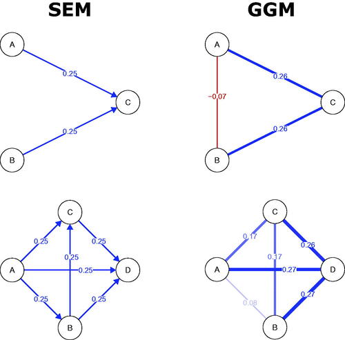
Figure 2. Visualization of the moral-equivalence set: A Pairwise Markov Random Field (PMRF) and the set of sufficient and faithful DAGs which generate that PMRF.

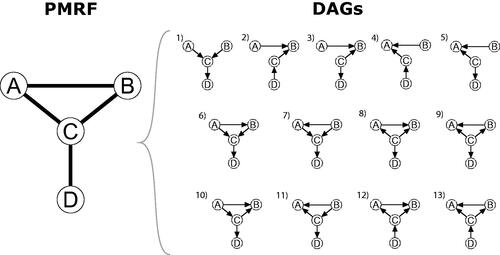
Formally, we could say that the PMRF identifies the moral-equivalence set of the underlying DAG: It allows us to find the collection of all DAG structures that produce the same moral graph, and hence the same PMRF. Generally speaking, many different DAGs share the same moral graph. In Figure 2 we show the moral-equivalence set for the four-variable burnout PMRF, derived using the discovery heuristics described above along with d-separation rules. The moral-equivalence set contains the DAG belonging to the true causal model, but also several other DAGs that match the PMRF structure equally well. In fact, in this example, 13 distinct DAG structures result in the same PMRF. Based on the PMRF alone, we cannot distinguish which of these is the true underlying causal structure.

Since the causal discovery heuristics described above only treat the causal information conveyed by individual edges in the network, researchers typically do not consider the causal information conveyed by the structure of the network as a whole, information that is directly conveyed by deriving and evaluating the moral-equivalence set. To illustrate how the latter may provide important information, consider Heuristic 1 which tells us that an edge in the PMRF might indicate a direct causal relationship or the presence of a collider structure. From Figure 2 we can see that there is at least one DAG in which either A and B, A and C, or B and C are causally independent of one another, and so are only connected in the PMRF due to the presence of a collider structure. However, by deriving the moral-equivalence set, we can see that this is never the case for the relationship between C and D: there is always a direct connection between these two variables. Since D is only connected to C in the PMRF, it cannot be the case that C and D share a common effect. In this instance, because of the overall structure of the PMRF, and the relationship between PMRF and DAG, we can say that C and D must share a direct effect. These types of deductions follow the same logic as the heuristics described above but follow from considering the graph as a whole, using the moral-equivalence set, rather than focusing only on individual edges in the network. By considering what combinations of relationships are and are not allowed by the PMRF we could gain more insight into the underlying causal structure. Using only the hypothesis-generation heuristics above, it is difficult to read off these global implications of the PMRF.

3.2. Limitations and Assumptions for Causal Discovery

While PMRFs can in principle be used for causal discovery in this way, it is important to note at least two caveats to such an approach. First and foremost, alternative causal discovery methods have been developed which will generally perform better in discovering DAG structures than the PMRF (Glymour et al., 2019; Scheines et al., 1998). Although most of these alternative methods also identify an equivalence set of DAGs from data, so-called constraint-based discovery methods, such as the PC algorithm (Spirtes et al., 2000) will typically yield a smaller, and so more informative, equivalence set than the PMRF.³ This happens because constraint-based methods typically test for a greater variety of independence relations between variables than are encoded by the PMRF. By testing for marginal and conditional independence relations given different subsets of the observed variables, the PC algorithm would, for instance, be able to distinguish between the first and second DAGs in Figure 2, since they imply different marginal independence relations between the variables A, B and C. By testing for different patterns of statistical dependence, so-called constraint-based causal discovery algorithms can also typically identify the direction of causal relationships whenever a collider structure is present (Scheines et al., 1998).

Second, the use of PMRFs for causal discovery in the manner outlined above is valid only under highly ideal circumstances. This means that even if the population PMRF is known, at least two additional assumptions are needed for the PMRF to yield valid inferences about the causal structure. These assumptions are well-known in the causal discovery literature and are shared with many constraint-based discovery methods, but their practical implications are not always easy to oversee. The first of these assumptions is known as sufficiency: Essentially the assumption that there are no unobserved “common cause” or “confounding” variables, that is, unobserved variables that cause two or more other variables in the network. These confounding variables would induce a statistical relationship between variables in the network while there is actually no causal relationship between them (Lauritzen, 1996; Pearl, 2009; Spirtes et al., 2000).⁴ In general, without this sufficiency assumption, the causal information conveyed by the presence of an edge (as stated in Heuristic 1) becomes uncertain. Relaxing the sufficiency assumption means that the task of causal discovery using network models becomes much more difficult, as, depending on the number and type of missing variables we are willing to consider, there are many more DAGs that could have generated the PMRF we obtained from the data.

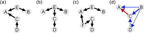
For example, consider that a single unobserved variable, E, could act as a common cause of A and B. Then, the DAG in Figure 3a needs to be considered as a plausible alternative underlying causal structure in addition to those in Figure 2. This DAG also produces the same conditional dependencies present between the observed variables A, B, C, and D as represented in the PMRF in Figure 2. In Appendix A we show that in fact nine additional causal structures must be considered if we allow only this exact type of unobserved common cause. If we relax the sufficiency assumption even further, for example allowing E to be a common cause of more than two variables, as in Figure 3b, or allowing more than one unobserved common cause as in Figure 3c, deriving a complete set of possible underlying DAGs quickly becomes infeasible. Hence, it is critical to evaluate the validity of the sufficiency assumption whenever we use conditional dependence information, such as those from a PMRF, to infer the presence of a direct causal relationship between variables.

Figure 3. Four DAGs which generate the same PMRF between the variables A, B, C, and D, as shown in Figure 2, but which violate some assumption which is made in deriving the moral-equivalence set. The DAGs in (a–c) represent sufficiency violations, with unobserved common cause(s) (E and F). The linear SEM in (d) violates faithfulness, as the directed positive relationship between B and D is exactly canceled out by conditioning on C.

The second major assumption needed to generate causal hypotheses using PMRFs is known as faithfulness (Pearl, 2009; Spirtes et al., 2000). Faithfulness is concerned with our ability to make inferences about the absence of a causal relationship between two variables in the face of the absence of a particular statistical relationship between those two variables. To be precise, a DAG and associated probability distribution P meet the faithfulness condition if and only if every conditional (in)dependence relation in P is entailed by the local Markov condition, as described in Equation (2)(2) $$X_i\hspace{0.17em}\perp \perp \hspace{0.17em}{\mathit{X}}_{-de(i)}\hspace{0.17em}|\hspace{0.17em}{\mathit{X}}_{pa(i)}.$$(2) (Spirtes et al., 2000). This implies that if, say, two variables X_i and X_j are marginally independent, then by faithfulness, the corresponding DAG should have no directed paths which can be traced from X_i to X_j, e.g. $X_i\to X_k\to X_j.$ This means that we assume away the possibility that X_i and X_j are connected by two different directed pathways, which when combined in the marginal relationship between X_i and X_j, exactly cancel one another out. For example, faithfulness would be violated if there was a negative direct pathway $X_i\to X_j$ as well as a positive indirect pathway of equal size through X_k. In general, without the faithfulness condition, the causal information conveyed by the absence of an edge (as in Heuristic 2) becomes less certain.

In Figure 3d we show a linear SEM which would result in a violation of faithfulness. In this causal system, both B and D have a positive direct effect on C, making it a collider between them. Conditioning on this collider C, which we do when estimating the PMRF, induces a negative conditional relationship between B and D. However, simultaneously, B has a positive direct effect on D: When combined, this negative and positive relationship cancel one another out, and so B and D appear to be conditionally independent given C—the partial correlation of B and D given C is zero, so they are unconnected in the PMRF (see Appendix A for details). Hence, it is crucial to evaluate the validity of the faithfulness assumption whenever we use conditional independence information to make inferences about causal independence between two variables (Spirtes et al., 1995).

Both of these assumptions, as well the general problems presented by the one-to-many mapping relating statistical to causal structures, are challenges which are shared across many different approaches to causal discovery. However, the specific details, limitations, and capabilities of other approaches differ from those of the PMRF as a discovery tool. In psychological research, the assumption of sufficiency may be unreasonable in many psychological settings (Rohrer, 2018). While some causal discovery methods have been adapted to deal with violations of sufficiency (Spirtes et al., 2000; Strobl, 2019; Zhang, 2008), it is unclear how the PMRF could be adapted in such a way, beyond adding a disclaimer that that network edges may actually only reflect the presence of unobserved common causes. As such, the two discovery heuristics commonly used in practice should be considered as describing what inferences can be made only in a highly idealized and likely unrealistic setting. In the following, we review the practice of using weighted PMRFs for the purpose of causal discovery, focusing on the case of the GGM, and consider what additional conditions are necessary for this approach to yield valid inferences about an underlying causal structure.

3.3. Causal Discovery with GGMs

The causal discovery heuristics considered above only describe inferences regarding the presence or absence of causal relationships based on the presence or absence of statistical relationships. Intuitively though, it would seem that more information about the underlying causal structure could be gleaned by using weighted networks, such as the GGM and Ising model. These models provide additional information by allowing us to consider the sign and strengths of different relationships, not only their presence or absence. However, the use of these models means applying additional assumptions about the functional form of the conditional dependence relationships between variables, and the probability distribution(s) of the variables involved. Violating these additional assumptions can also lead to erroneous conclusions: For instance, if the true causal relationship between two variables is non-linear, they may produce a zero partial correlation in the GGM, which could, in turn, lead to incorrect inferences regarding the absence of a causal relationship between those variables.

Here we will focus on the use of the GGM as a causal discovery tool in the situation where all of these additional statistical assumptions are met. Specifically, we’ll consider the variables involved to have a joint Gaussian distribution, and the causal relationships to be linear. This means we can view the true underlying causal structure as an SEM, as presented in Equation (3)(3) $$\mathit{X}=\mathit{\alpha }+\mathit{BX}+\mathit{ϵ}$$(3) . The weights matrix of the GGM can be related to the matrix of direct effects in an SEM model by noticing that both models represent decompositions or transformations of the variance-covariance matrix of the observed data, denoted $\mathbf{\Sigma }.$ Recall that the GGM consists of partial correlations between variables. This matrix of partial correlations can be obtained by estimating and re-scaling the inverse of the variance-covariance matrix ${\mathbf{\Sigma }}^{-1}$ (Epskamp, Waldorp, et al., 2018). From the SEM literature, it is known that the following expression relates the parameters of an SEM to the variance-covariance matrix of the data (4) $$\mathbf{\Sigma }={(\mathit{I}-\mathit{B})}^{-1}\mathbf{\Psi }{(\mathit{I}-\mathit{B})}^{-T}$$(4) where $\mathbf{\Psi }$ is the residual variance-covariance matrix of the variables X, which is diagonal if these residuals are uncorrelated (Bollen, 1989). These two expressions together can be used to determine how a linear SEM model maps onto the GGM, and hence how the network functions as a causal discovery method under the most ideal conditions possible.

The relationship between the GGM and the linear SEM model has many of the same implications for causal discovery as those of the PMRF and DAG relationship we reviewed above (Epskamp, Waldorp, et al., 2018). First, if the assumption of sufficiency holds, then the presence of an edge in the GGM will correspond to either the presence of a weighted edge in the SEM model or the presence of a collider structure. Second, the absence of an edge in the GGM may in many situations correspond to the absence of an edge in the true path model, but this is not always necessarily the case (a point we elaborate on further below). The most important implication of this is that also in this scenario, multiple true underlying causal SEMs may result in the same GGM. As we noted earlier, there are typically many different SEM models which are statistically equivalent to one another, which implies that there are many different sets of regression parameters B that can produce the same variance-covariance matrix $\mathbf{\Sigma }$ (MacCallum et al., 1993; Raykov & Marcoulides, 2001), and hence the same matrix of partial correlations.

We can understand the utility of the GGM as a causal discovery tool by deriving this set of statistically-equivalent models from the GGM weights, much as we did in the previous section for the PMRF. Although this process is a little more involved than for the moral-equivalence class in the previous section, we have developed a relatively simple algorithm that allows researchers to do this, described in Appendix B and which is available as an R package SEset from the comprehensive R archive network (CRAN: Hornik, 2012; R Core Team, 2021). In Figure 4 we show our example burnout GGM along with all of the linear SEM models which reproduce that GGM, in other words, the statistical-equivalence set for that network. To obtain this set we assume sufficiency, that is, we only consider path models which consist of the same set of variables as those in the GGM (i.e., no unobserved confounding variables). We do not need to assume faithfulness in deriving this equivalence set, the implications of which we discuss further below. Note that the statistical equivalence set does contain the true data-generating SEM model, but that this is only one of many possibilities, and this true model cannot be distinguished from other qualitatively different SEM models based on the GGM alone.

Figure 4. A Gaussian graphical model (GGM) and the set of linear SEM models which generate that GGM.

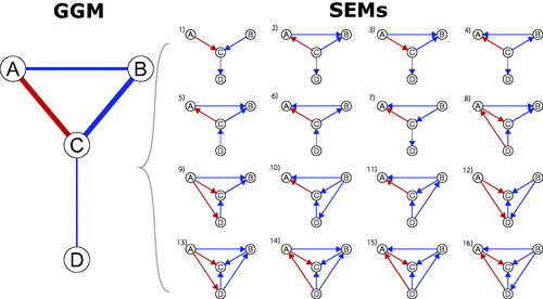
Using information about the sign and strength of the partial correlations, in combination with the linearity and normality assumptions outlined above, allows us to gain much more information about the underlying causal structure than when considering only the presence or absence of conditional dependence, given that these assumptions are correct. Comparing the statistical equivalence set to the moral-equivalence set in Figure 2, we can see that the weighting information allows us to rule out unweighted DAGs numbered two through seven in Figure 2. For example, the moral-equivalence set considers a DAG in which A and C are causally independent but share a collider B ($A\to B\leftarrow C$) to be a valid possibility, based only on the presence of conditional dependence between these three variables in the PMRF. Utilizing the model assumptions, the statistical-equivalence set rules out this possibility: It isn’t possible to define a linear Gaussian SEM model where A and C are causally independent, but which still produces the exact partial correlations in the given GGM.

However, as well as ruling out certain possibilities, the statistical-equivalence set also contains weighted causal structures which do not correspond to any DAG which appears in the moral-equivalence set (i.e., SEMs number eight through sixteen). For example, SEM ten in Figure 4 contains a small positive direct effect $B\to D$ even though the partial correlation of B and D, conditioning on both A and C, is zero in the GGM. The reason for this discrepancy is that to obtain the moral-equivalence set we needed to assume faithfulness, while we did not need to do this to derive the statistical-equivalence set. By using the information in the partial correlation matrix directly, we can derive different possible linear SEMs in which conditioning results in approximately zero partial correlations between variables. As a consequence, we consider different potential causal structures that violate the faithfulness assumption in the statistical-equivalence set, which were not considered in the moral equivalence set. This is desirable, because the faithfulness assumption may not always be reasonable in the context of sampled data, as we discuss below.

3.4. Limitations to GGM-Based Causal Discovery

The partial correlations in the GGM aid causal discovery by supplying the information necessary to derive the statistical equivalence set. However, outside of the statistical-equivalence set, partial correlations cannot be used to make straightforward inferences about the size of the underlying causal effects: The mapping between linear SEM and GGM model does not guarantee that say, the largest partial correlation also reflects the largest causal relationship. In Figure 4 the partial correlations $A-C$ and $B-C$ are the strongest edges in the GGM, being of opposite signs but having the same absolute value. However, the relative size of the corresponding direct effects in the underlying causal model varies depending on the structure of the underlying causal model. In only six of the SEM models in Figure 4 are the corresponding direct effects equal in size (models one and twelve through sixteen); in five of these models the direct effect linking B and C is larger (models two, three, five, eight and nine) and in the remaining five (models four, six, seven, ten, eleven) the direct effect between A and C is largest.⁵ As such, inferences about the size of causal effects based directly on the size of partial correlations in the GGM should, in general, be avoided.

Here we showed that by considering the GGM as a causal discovery tool for a linear and acyclic SEM model, and evaluating which of the necessary assumptions we find acceptable in a given situation, we can gain insights into the underlying causal system. However, as we saw in the case of the PMRF, the causal discovery heuristics used in the network literature provide only a limited account of how this works in practice. To appropriately use these tools for causal discovery, it is essential to consider the graph as a whole, and the equivalence set of causal structures which that graph represents. Moreover, as was the case for the PMRF, to use the GGM to generate causal hypotheses, it is essential to consider what type of causal structure we are trying to learn about, and what assumptions we need and can reasonably make about that causal structure. Furthermore, note that for both the statistical and moral-equivalence set, as the number of nodes and/or connections in the graph grows, generally speaking so too does the size of the equivalence set. The implication of this is that making inferences about the causal structure of the directed graph becomes more and more difficult because more and more equivalent causal structures will lead to the same statistical network, even under ideal conditions where all our assumptions are valid.

3.5. Estimated Network Models and Causal Discovery

So far, we have only considered the principles of using statistical network models for causal discovery using the relationship between the population network model and the underlying causal structure. Of course, in practice, researchers also must contend with the uncertainty that results from estimating a particular network from sample data. This further complicates the task of using statistical networks for causal discovery in practice, because researchers must deal with additional concerns and make more assumptions and decisions beyond those discussed earlier. For instance, to estimate the PMRF structure, researchers will typically have to choose some method to statistically test for conditional independence between variables (e.g., with a significance test), which may depend on additional assumptions next to those of the statistical model used to estimate the graph weights.

Generally, researchers must contend with the inherent uncertainty in their parameter estimates, that is, uncertainty about how closely the estimated network model parameters reflect the population network. This uncertainty could be accounted for in many ways, for example by considering standard errors, bootstrapping the network, or by sampling different network models from the posterior in a Bayesian approach (Epskamp, Borsboom, et al., 2018; Williams & Mulder, 2020a, 2020b). However, the uncertainty will almost surely lead to considering an even larger set of possible data-generating structures than when the population network is available.

The role of parameter uncertainty is also crucial for the validity of the assumption of faithfulness. Faithfulness may be a reasonable assumption regarding the presence of exact zero dependencies in the population since it would seem unlikely that in the true causal system relationships perfectly cancel out such that a population statistical dependency becomes exactly zero. So, if the GGM in Figure 4 would be the population network structure, we may consider it reasonable to rule out SEMs eight through sixteen as plausible data-generating structures, since these would constitute a violation of faithfulness. However, if the GGM is an estimate of the population network structure, then we may not be so quick to rule out these possibilities.

When estimating a network model, researchers typically use either a decision rule (such as a threshold value or significance test) to set certain edge weight estimates to zero or use regularization techniques to obtain a sparse network, that is, a weights matrix that contains exact zero values (Epskamp & Fried, 2018; Williams & Rast, 2020; Williams et al., 2019). When using an unbiased estimation technique in combination with significance tests, researchers should be cognizant of type II errors, meaning that they may fail to reject the null hypothesis that a particular edge weight is zero, even though it is non-zero in the population. The popular use of regularization techniques, such as the lasso (Epskamp & Fried, 2018; Friedman et al., 2008) bears even closer consideration in the context of causal discovery. The lasso works by inducing bias in the parameter estimates such that small edge weights are set to zero, meaning that even if the true population parameter is small enough then regularized estimation techniques would be expected to return an exact zero value for that parameter across samples. The upshot is that, even if we are willing to assume faithfulness with respect to the population, the absence of an edge in an estimated network model may not reflect the absence of an underlying causal relationship (Tzelgov & Henik, 1991; Uhler et al., 2013). This represents a challenge to the practical application of network models for causal discovery since seemingly unfaithful causal models should not be ruled out based on an estimate of the network model.

3.6. Intermediate Summary

Statistical network models can be understood as causal discovery tools which allow for inferences about particular equivalence classes of directed causal structures. The PMRF can be understood as identifying the moral-equivalence class of an underlying DAG, as long as the assumptions of sufficiency and faithfulness hold. This characterization of the PMRF is consistent with the heuristics for causal hypothesis generation proposed by network methodologists. If we additionally assume that the causal structure consists of linear relationships between variables with a Gaussian distribution and that sufficiency holds, then we can also characterize the GGM as a causal discovery tool. Specifically, the GGM would then identify the statistical-equivalence class of an underlying linear SEM model. In the following, we consider various implications of the relationship between network models and underlying causal models that we have discussed above and use this to dispel four common misconceptions which present in the empirical literature regarding the causal interpretation of network parameters.

4. Common Misconceptions

In the previous section, we have outlined the properties of network models as causal discovery tools. However, there are several implications of those properties that are not immediately obvious, but which have direct implications for how these models are used in practice. In the following, we will tackle four different misconceptions in the applied literature around statistical network models, which we believe have arisen due to a lack of clarity around how these models operate as causal discovery tools. These misconceptions concern (1) the interpretation of networks as causal skeletons, (2) the use of network heuristics to infer multivariate patterns of causal relationships, (3) the effect of collider variables on the size and sign of network edges, and (4) “causal agnosticism” and the possibility of using network models to discover cyclic causal relationships.

4.1. Causal Skeletons and Spurious Edges

As outlined above, the PMRF can be interpreted as the moral graph of an underlying DAG. Crucially, the moral graph of a DAG should not be confused with the skeleton of a DAG. The skeleton of a DAG is the undirected graph obtained by replacing the directed edges in a DAG with undirected edges: The skeleton contains an edge between two nodes if and only if the underlying DAG contains an edge between those nodes (Spirtes et al., 2000). The skeleton describes exactly which variables do and do not share a connection, but does not contain information on the directionality of that connection. In general, the moral graph will contain more edges than the skeleton, with additional edges induced in the moral graph whenever there is a collider with unmarried parents. The difference between the moral graph (PMRF) and the skeleton is shown for three example DAGs in Figure 5. We see that although all three DAGs share the same skeleton, each moral graph is distinct. If we interpret the DAG in causal terms, we can see that variables can be statistically dependent in the PMRF even while they are causally independent in the corresponding DAG: In both the first and third row of Figure 5, A and D are conditionally dependent given C (there is an edge A–D in the PMRF), but intervening on A has no effect on the value of D or vice versa.

Figure 5. Three examples of DAGs which all have the same skeleton, but result in different moral graphs depending on the orientation of the edges in the DAG.

While many researchers correctly describe the relation between PMRF and DAG (Borsboom & Cramer, 2013; Epskamp, Waldorp, et al., 2018), the term “causal skeleton” is occasionally used to describe the PMRF (e.g. Armour et al., 2017; Borsboom & Cramer, 2013; Fried et al., 2016; Haslbeck & Waldorp, 2018; Isvoranu et al., 2017; van Borkulo et al., 2015), which can easily lead to confusion regarding the causal status of edges in statistical network models. For example, researchers may be tempted to interpret that, by statistically controlling for all other variables, the statistical dependencies in the network have filtered out all “spurious” relationships (Rohrer, 2018; Spector & Brannick, 2011) thereby producing a causal skeleton. The idea that networks filter out certain uninteresting relationships is often emphasized in the network literature: Costantini et al. (2015) point out that conditioning on all other variables has the effect of omitting “spurious” connections in the sense of eliminating marginal dependencies produced by mediation or common cause pathways but which do not reflect direct causal connections. For instance, in the bottom row of Figure 5, the path $A\to C\to B$ implies that A and B are marginally dependent ($A\cancel{\perp \perp }B$), although there is no direct effect between them, and we can see that the PMRF correctly omits any $A-B$ edge. Importantly, however, it is also true that by conditioning on all variables, we will typically also induce spurious relationships by conditioning on colliders, as we can see from the $A-D$ edge in that very same network.⁶

4.2. Multivariate Patterns in PMRFs and Causal Chains

Although the two heuristics which are used for causal discovery with network models correctly describe how any individual edge can be interpreted, they fail to communicate information about the global structure of different possible underlying causal systems. However, it is clear from the empirical literature that very often researchers are interested in making inferences about (parts of) the global structure of the system, not just individual edges. One example of this is the common practice in empirical papers of interpreting a chain of dependent variables in a PMRF, of the form $X_i-X_j-X_k$ as indicative of a directed mediation structure, $X_i\to X_j\to X_k,$ interpretations which are present in, for example, Deserno et al. (2017) ($X_i=$ social contacts, $X_j=$ social satisfaction, $X_k=$ feeling happy), Isvoranu et al. (2017) ($X_i=$ sexual abuse, $X_j=$ anxiety and depression, $X_k=$ psychosis) and Fried et al. (2015) ($X_i=$ bereavement, $X_j=$ lonely, $X_k=$ sad and happy). These types of interpretations may be reasonable in many cases but are prone to error if they are made without considering the appropriate equivalence set, that is, the moral- or statistical-equivalence sets we have described in the current paper. The reason for this is that combinations of different causal hypotheses based on individual edges may be incompatible with one another, as they may imply, for example, a new collider structure, or some (in)dependence relationships that either contradict those in the PMRF or which are otherwise not present in the population.

In Figure 2 for example, we may be tempted to interpret the PMRF as showing a pattern of dependencies consistent with the hypothesis that A has a direct effect on B ($A\to B$), as well as an indirect effect through C ($A\to C\to B$). Let us call this hypothesis I. To take another example, a researcher may be tempted to hypothesize that, as there is no connection between D and B, this is indicative that the effect of D on B is fully mediated by the variable C, that is $D\to C\to B.$ Let us call this hypothesis II. Inspecting Figure 2 we can see that hypothesis I holds in only one of thirteen DAG structures, DAG number 10. Furthermore, hypothesis II holds in exactly three DAG structures, numbers 2, 12, and 13. Strikingly, hypothesis I and II are totally incompatible with one another: although both hypotheses are reasonable explanations of two different local structures, and in fact hypothesize the same direction for one edge $C\to B,$ it is impossible for both to be true in any of the underlying DAG structures that correspond to the given PMRF. Thus, if researchers use the hypothesis-generation heuristics to make inferences about individual edges, they may be correct under the conditions outlined above. But, if they try to combine these inferences to say something about causal chains or global structures, they may easily come to erroneous conclusions.

4.3. Colliders, Negative Edges, and the Positive Manifold

As we have outlined above, the size and sign of edges in networks such as the GGM may not reflect in a straightforward way the value of a corresponding direct effect in the causal system being studied. Discussions of this general phenomena in the applied literature, however, are often limited to one very specific consequence of conditioning on a specific kind of collider structure: if we assume a so-called “positive manifold” of causal relationships, then small negative edges might be induced in the network due to collider conditioning (as discussed by Betz et al., 2021; Black et al., 2021; Epskamp, Waldorp, et al., 2018; Hoffman et al., 2019; Isvoranu et al., 2020).

In clinical psychology, the positive manifold refers to the observation that symptoms of a disorder are typically positively correlated, and one popular explanation for the positive manifold is that the underlying causal system consists only of positive (activating) relationships between nodes (Borsboom et al., 2011; van Bork et al., 2017; Van Der Maas et al., 2006). From the causal modeling literature, it is known that when two causally independent parents both exert a positive linear influence on a collider variable (a positive collider), then conditioning on that collider will induce a negative statistical dependency between those variables (for details see Greenland, 2003; Jiang & Ding, 2017; Nguyen et al., 2019; Pearl, 2013). An example is shown in the top row of Figure 6 where, although A and B are causally independent in the underlying linear causal model, there is a negative partial correlation between them conditional on the collider C.⁷ Taken together, this means that, if we are willing to assume that there is a positive causal manifold, then small negative edges in the statistical network may be interpreted as spurious, in the sense that they are induced by collider conditioning, and not reflective of the presence of a direct causal effect (Betz et al., 2021; Black et al., 2021; Epskamp, Waldorp, et al., 2018; Hoffman et al., 2019; Isvoranu et al., 2020).

Figure 6. Two examples of linear SEMs and their corresponding GGM.

However, it would be incorrect to think that this is the only undesirable consequence of collider conditioning, or that the presence of colliders can always be detected in such a straightforward way, even if we assume a positive manifold. A more precise formulation of this type of collider bias is that when we aim to estimate the direct causal dependency between a pair of variables sharing a positive collider, conditioning on that collider introduces a negative bias in our estimate of that causal effect. However, this negative bias does not necessarily result in a small negative edge in the network. Instead, this bias can produce, in a general sense, highly inaccurate inferences about the strength and size of causal relationships based on the strength and size of the statistical network relationships.

We further illustrate the implications of negative collider bias for network research with a simple example: The bottom left-hand panel of Figure 6 depicts a linear SEM model reflecting a system that exhibits the positive causal manifold, and where the positive standardized regression weights are all exactly equal in magnitude. In other words, every single direct effect in the system is exactly equal in strength: increasing A by one unit has the exact same positive direct effect on B, C, and D, and so forth for all other direct effects in the system. However, when we derive the corresponding GGM for this system in the bottom right-hand panel, we obtain a network with a range of different edge weights. Here, the edge between A and B is much smaller than that between A and C, which is again smaller than the edge connecting A and D. The asymmetry in edge weights in the GGM is produced by the differential effects of collider bias. Since A and B share two positive colliders, their GGM edge weight experiences a greater degree of negative bias than the edge weight between A and C, while the edge weight between A and D could be considered unbiased since those variables do not share any colliders in the SEM. Researchers presented with this GGM may be tempted to interpret that A and B have only a very weak direct effect on one another, while D shares much stronger direct effects with all other variables in the network. Perhaps researchers would even conclude that D is an attractive intervention target since it has relatively high direct effect centrality (Bringmann et al., 2019; Robinaugh et al., 2016). However, in this instance, all such conclusions would be patently incorrect, since, in the true causal system, all direct effects are exactly equal.

In the general case, the degree of collider bias present in any edge weight depends on the number of colliders present as well as the strength of the individual effects which make up that collider structure. This means that in the general case, without any knowledge of the direction of effects, the presence and degree of collider bias is difficult—if not impossible—to detect from the statistical network structure alone. As we saw above, this has obvious implications for researchers who attempt to interpret the magnitude of edge weights in a statistical network, or who attempt to calculate metrics like density and centrality, which are direct functions of those edge weights. Since network edge weights may be very different from their corresponding causal relationships, even when a positive manifold can be assumed, the network edge weights may produce a misleading account of the causal relationships in the system (see also Dablander & Hinne, 2019). Even if the presence of a network edge does reflect the presence of a causal effect, the value of the network edge should not in general be taken as an estimate of that causal effect.

4.4. Causal Agnosticism and Causal Cycles

Although we have focused on characterizing the utility of statistical network models as DAG discovery tools, it is also clear from the literature that many network researchers explicitly reject the idea that the underlying causal structure of interest can be represented by a DAG. In fact, many researchers adopt what could be called a causally agnostic approach: leaving unspecified whether the causal structure contains uni-directional or bi-directional relationships, or whether the structure is cyclic or acyclic (Costantini et al., 2015; Cramer et al., 2010; Epskamp, Waldorp, et al., 2018; Isvoranu et al., 2017; McNally et al., 2015; Robinaugh et al., 2016; Van Borkulo et al., 2014). This state of affairs presents an obstacle to assessing the utility of statistical network models for causal discovery since this agnosticism leaves it unclear how we could go about such an assessment. That is, without specifying the type of causal structure we wish to discover, it is unclear whether the heuristics used to conduct causal discovery are actually valid. To make a statistical analogy, it is impossible to evaluate the properties of a given estimator if we never specify what the target of inference (i.e. the estimand) actually is (Haslbeck et al., 2021a).

One reason why researchers reject the DAG as a model for the underlying causal structure is that the DAG by definition does not allow for the presence of causal loops, that is, directed cyclic causal relationships, such as $A\to B\to C\to A$ or $A\leftrightarrows B.$ In substantive terms these causal loops would represent feedback relationships: Feeling more stressed leads you to worry more which in turn leads you to feeling more stressed. One argument for using PMRF based methods to learn about cyclic causal models was made by Epskamp et al. (2017), who correctly point out that PMRF models can represent certain conditional dependence structures that can be produced only by cyclic, rather than acyclic graphs, as shown in the top row of Figure 7. It has been shown that d-separation rules can be applied to cyclic as well as acyclic graphs in the linear and discrete case (Pearl & Dechter, 1996; Spirtes, 1994), which means that, in principle, the two causal discovery heuristics described above can also be used in this setting. In general, however, if we are willing to consider possibly cyclic causal structures, then using PMRF models for causal discovery will typically become more difficult than if we limit ourselves to considering DAGs, since in many situations the challenges and problems with this approach, as have outlined above, will be exacerbated rather than mitigated.

Figure 7. Two examples of directed cyclic graphs (DCGs) and their corresponding PMRF.

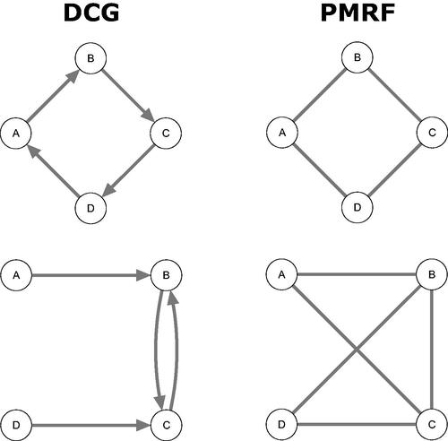
When aiming to discover cyclic causal graphs, considerations of faithfulness and sufficiency are still critical, but allowing for cycles means that the size of the equivalence class of causal models which produce the same PMRF will typically become even larger and more difficult to derive than in the acyclic case. Allowing for bi-directional causal relationships by necessity increases the number of potential collider structures, as shown in the example in the bottom row of Figure 7. Here, B and C each have a direct effect on one another, meaning that we have two collider structures, $A\to B\leftarrow C$ and $B\to C\leftarrow D.$ As a result, the PMRF of this system contains two new edges induced by conditioning on a collider. Even when no new edges are induced, the possibility for more collider structures means a greater potential for collider bias impacting the edge weights in weighted networks in undesirable ways, as described above. Allowing for asymmetric pairs of direct effects between variables also raises new difficulties for the interpretation of network models: If in our example the $B\to C$ effect isn’t equal to the $B\leftarrow C$ effect, how should the partial correlation between those variables in a GGM be interpreted? It’s possible that statistical network models are still valuable tools to study cyclic causal systems, but researchers should be aware that the limitations and pitfalls of using these models as DAG discovery tools, as outlined in this paper, carry over to the context of using network models to discover cyclic causal relationships too.

5. Discussion

With this paper, we aimed to clarify the role of statistical network models as tools for causal discovery. We believe that causal discovery accurately characterizes the common practice researchers engage in when they attempt to “generate causal hypotheses” from an estimated network model. We formalized how network models can in principle be used to that end, showing how network models can be used to identify equivalence classes of directed acyclic causal structures. We outlined the advantages and disadvantages of this approach and described the key assumptions necessary for causal discovery using statistical networks. We addressed several misconceptions which appear in the network modeling literature regarding the interpretation of networks as causal skeletons, inferences about multivariate patterns of causal relationships, the effects of collider bias and the status of edge weights as estimates of causal effects, and finally the utility of networks for learning about cyclic causal models. We believe awareness of the issues raised in this paper is critical for the growing group of researchers who wish to use statistical networks to gain insights into–that is, generate useful hypotheses about—causal structures (Robinaugh et al., 2020).

We emphasized that the utility of any causal discovery method depends on the validity of assumptions we make about the underlying causal structure. Ironically, the more specific knowledge we have about the nature of the causal system, the less likely it becomes that the PMRF or GGM is the optimal causal discovery method to use, unless of course that system is made up of symmetric and undirected causal relationships (Cramer et al., 2016; Dalege et al., 2016). Moreover, it is important to note that alternative causal discovery tools which are built for purpose are generally likely to outperform statistical network models. Several causal discovery methods have been developed which aim to uncover causal structure using patterns of conditional independence between variables (Ramsey et al., 2017; Scheines et al., 1998; Spirtes et al., 2000), each leveraging different assumptions about the causal system, and each coming with their own advantages and disadvantages. For instance, some of these approaches can deal with violations of sufficiency in the estimation of the equivalence class (Colombo et al., 2012; Richardson & Spirtes, 2002; Spirtes et al., 2000); others leverage assumptions about the functional form of variable relations (Mooij et al., 2016; Peters et al., 2010) or the distribution of noise terms (Shimizu, 2014; Shimizu et al., 2006) to uniquely identify the causal graph from observational data. Yet other approaches make use of a mix of observational and intervention data to identify parts of the underlying causal graph (Kossakowski et al., 2021; Mooij et al., 2016; Peters et al., 2016; Waldorp et al., 2021). For an accessible overview of recent causal discovery methods, we refer readers to Glymour et al. (2019).

Of course, while most causal discovery methods focus on the discovery of DAG structures, those methods may not be appropriate when the underlying causal structure consists of cycles or feedback loops between variables. As we have outlined above, the limitations of PMRF-based methods for acyclic causal discovery carry over to the cyclic case, where issues such as collider bias are likely to be exacerbated. Discovery methods for cyclic causal models have also been developed (e.g., Forré & Mooij, 2018; Hyttinen et al., 2012; Lacerda et al., 2012) but to our knowledge, their applicability in typical psychological settings has yet to be studied. The consideration of cyclic causal models, in general, presents new difficulties not present in the acyclic case. For example, in the SEM literature, it is well-known that, in contrast to acyclic models, not all cyclic models are statistically identifiable from data (Bollen, 1989). More research into the semantics of cyclic causal graphs and how they could be applied in a psychological setting is urgently needed.

Outside of their use for causal discovery, there are many attractive reasons to use statistical network models. The Ising model, for example, has been used as a theoretical toy model, describing a causal system with fully symmetric causal relationships (Cramer et al., 2016; Dalege et al., 2016). Statistical network models are also useful as descriptive tools, to explore and visualize multivariate statistical relationships; they allow for the identification of predictive relationships (Epskamp, Waldorp, et al., 2018); provide sparse descriptions of statistical dependency relationships in a multivariate density; and may be used as a variable clustering or latent variable identification method (e.g. Golino & Epskamp, 2017). These useful characteristics suggest that PMRFs estimated from psychological data might best be viewed as phenomena to be explained by some theoretical model of psychopathology, rather than as a tool to discover causal relationships in an inductive fashion (Haslbeck & Ryan, 2021; Haslbeck et al., 2021b; Robinaugh et al., 2021).

In sum, if the network approach to psychopathology is to make progress in the hunt for causal mechanisms underlying psychological disorders, further development of both theoretical modeling approaches and causal discovery methods suitable to a psychological context is in dire need. We hope that the treatment presented in the current paper helps to clarify the role that statistical network models might play in that hunt moving forward.

Additional information

Funding

The work of Oisín Ryan was supported by a grant from the Netherlands Organization for Scientific Research (NWO; Onderzoekstalent Grant 406-15-128).

Notes

1 Note we consider only the structural equation here, omitting the measurement equation. SEM models without measurement equations are sometimes referred to as path models.

2 A collider structure $X_i\to X_k\leftarrow X_j,$ which does not contain an edge directly connecting the parents ($X_i\nrightarrow X_j$ and $X_i\nleftarrow X_j$) is called an open v-structure. If there are any open v-structures in the DAG, then the moral graph must contain an undirected edge between the relevant parents $X_i-X_j.$ Thus, the moral graph “marries” unmarried parents.

3 The PC algorithm identifies the Markov-equivalence set of a DAG, the set of DAGs that satisfy the same d-separation statements and which match the independence relations between variables in the data.

4 Formally, there are no unblocked back-door paths, based on d-separation rules, passing through unobserved variables, that connect any pair of observed variables (Pearl, 2009).

5 The example GGM and all of the SEM model weights matrices in the statistical-equivalence set can be found in the supplementary materials of this paper: https://osf.io/qfyx9/.

6 Notably, there are other reasons not considered here why relationships in a statistical network can be considered spurious or biased estimates of an (in)dependence relationship, which are not eliminated via conditioning. For example, measurement error can result in under- or over-estimation of partial correlation relationships relative to those present between the true constructs of interest (c.f., Buonaccorsi, 2010; Schuurman & Hamaker, 2019).

7 Let ρ_AC represent the correlation between A and C and let ρ_BC represent the correlation between B and C. If C is a positive collider in a linear SEM model, then ρ_AC and ρ_BC lie between zero and one in value. Take it that A and B are causally independent, as in the top right panel of Figure 6. Following Pearl (2013), the partial correlation between A and B conditional on C is given by $\frac{-{\rho }_{AC}{\rho }_{BC}}{\sqrt{(1-{\rho }_{AC}^2)(1-{\rho }_{BC}^2)}},$ which, given the aforementioned range restriction, will be negative.

Appendix

A. Moral-Equivalent DAGs: Violations of Sufficiency and Faithfulness

In this Appendix we provide additional insight into moral-equivalent DAGs which violate the assumptions of either sufficiency or faithfulness.

A.1 Sufficiency-Violating DAGs

In the main text, Figure 3a, we show a single example of a DAG which generates the PMRF depicted in the left-hand column of Figure 2, in the presence of an unobserved variable E which acts as a common cause of both A and B. If this is the data-generating DAG, we can say that variables A–D do not meet the assumption of sufficiency—to derive the true DAG, the variable E is needed.

If we assume that sufficiency is violated only in that an unobserved variable E is a common cause of A and B, then there are eight more DAGs which generate the same PMRF for the variables A–D, and contain one less directed edge between the variables A–D than any of the DAGs in the moral-equivalent set shown in the right-hand column. These are depicted in Figure 8. Many more moral-equivalent DAGs are possible if the assumption of sufficiency is relaxed further, that is, if different and/or additional connections between E and other variables or allowed, or if more than one unobserved common cause is allowed.

Figure 8. Eight additional DAGs which generate the same PMRF between the variables A–D (as shown in Figure 2). For each DAG, the set of variables A–D violates the sufficiency assumption, with respect to the variable E, a common cause of both A and B.

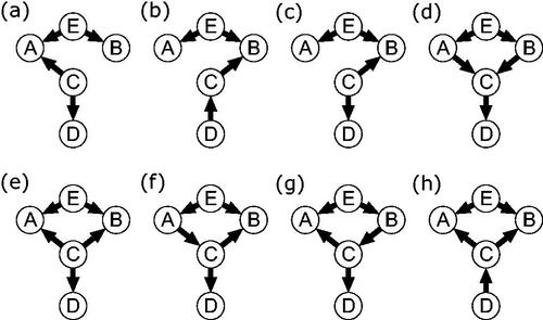
A.2 Faithfulness-Violating Weighted DAGs

In the main text, Figure 3d, we depict a linear SEM which generates the PMRF depicted in the left-hand column of Figure 2, but which violates the faithfulness assumption. The weights matrix of this linear SEM is given as (5) $$\mathit{B}=\left[\begin{array}{cccc}0.000& 0.200& -0.400& 0.000\\ 0.000& 0.000& 0.000& 0.000\\ 0.000& 0.485& 0.000& 0.152\\ 0.000& 0.100& 0.000& 0.000\end{array}\right]$$(5) Although there is a positive direct effect from B to D, denoted by the parameter $b_{42}=0.100,$ the correlation between B and D when C is conditioned on is zero. This is because conditioning on C induces a slight negative relationship between B and D, which cancels out the positive directed effect from B to D.

It is well-known that if two variables X and Y are independent but share a collider Z on which both have a positive linear effect, there will be a negative partial correlation between X and Y conditional on Z (cf. VanderWeele & Robins, 2007). Suppose X and Y are standard normal variables, and fully determine the variable Z, both having the same positive effect on Z. Now consider that we condition on Z taking on its average value, Z = 0. If we also know that X takes on a moderately low value (say, $X=-0.5)$ then it must be the case that Y takes on a high value (Y = 0.5)—otherwise, it would not be possible for Z to take on a value of zero. In this way, although both X and Y are causally independent, if we know the value of their common effect Z, then X and Y contain information which can be used to predict one from the other.

B. Statistically Equivalent SEMs from GGMs

In this Appendix we describe a tool which allows us to directly relate a given GGM to a set of causal structures with linear functional relationships and Gaussian noise terms, i.e., linear SEM models. This tool takes as input an (estimated) precision matrix or partial correlation matrix and outputs a set of linear path models structures between the observed variables. While each of these path models may lead to very different substantive interpretations, they all lead to the same pattern of partial correlations between the observed variables described by the GGM. We can say that they are statistically-equivalent in the sense of a structural equation model, in that they produce the same model-implied variance-covariance matrix (Bollen, 1989; MacCallum et al., 1993; Raykov & Marcoulides, 2001; Tomarken & Waller, 2003). This tool is thus called the statistical-equivalence-set or SE-set algorithm. The current implementation is limited to deriving path models which meet the sufficiency assumption. However, since we utilize SEM matrix relationships to derive the SE-set, rather than a constraint-based causal discovery method (Pearl, 2009; Spirtes, 1995) it is not necessary to invoke the faithfulness assumption, and so the SE-set algorithm may produce DAGs which are unfaithful to the set of conditional (in)dependencies described by the GGM. For a similar method that is able to discover unfaithful DAG structures from data see Ghoshal and Honorio (2017). Note that the SE-set algorithm is intended primarily as an illustrative and exploratory tool.

The weights matrix of the $p-$ variate GGM and the weights matrix of a linear SEM can be related to each other through the p × p inverse variance-covariance matrix, known as the precision matrix $\widehat{\mathbf{\Omega }}.$ (6) $$\mathbf{\Sigma }={\mathbf{\Omega }}^{-1}.$$(6) The weights matrix of a weighted DAG was defined in Equation (3)(3) $$\mathit{X}=\mathit{\alpha }+\mathit{BX}+\mathit{ϵ}$$(3) as the matrix of regression parameters B in which child variables are regressed on their parents. In other words, a linear SEM model with uncorrelated residual terms can be treated as a weighted DAG. From the SEM literature, there is a straightforward expression relating the parameters of such a path model to a model-implied variance covariance matrix. (7) $$\mathbf{\Sigma }={(\mathit{I}-\mathit{B})}^{-1}\mathbf{\Psi }{(\mathit{I}-\mathit{B})}^{-T}$$(7) where $\mathbf{\Psi }$ is a matrix of residual variances of X, diagonal in the case of uncorrelated residuals (Bollen, 1989). As such, the weights matrix of both the GGM and the linear SEM can both be seen as decompositions of some variance-covariance matrix $\mathbf{\Sigma }.$

We use this relationship to define the SE-set algorithm. If $\mathbf{\Psi }$ and B are both known, then they can be combined to find $\mathbf{\Sigma }$ using Equation (7)(7) $$\mathbf{\Sigma }={(\mathit{I}-\mathit{B})}^{-1}\mathbf{\Psi }{(\mathit{I}-\mathit{B})}^{-T}$$(7) . However, the inverse operation, solving uniquely for B and $\mathbf{\Psi }$ from $\tilde{\mathbf{\Sigma }}$ is not typically possible without additional information or assumptions. It is possible to find B directly from the covariance matrix when the topological ordering of the DAG is known, and the residual terms are assumed to be uncorrelated (Levina et al., 2008; Shojaie & Michailidis, 2010). The topological ordering of a DAG is an ordering of nodes such that every parent comes before every child. The graph in Figure 1c has two valid topological orderings: $\{$Support, Pressure, Stress, Worry$\}$ and $\{$Pressure, Support, Stress, Worry$\}.$ If the rows and columns of the covariance matrix $\mathbf{\Sigma }$ are sorted according to the topological ordering, then Equation (7)(7) $$\mathbf{\Sigma }={(\mathit{I}-\mathit{B})}^{-1}\mathbf{\Psi }{(\mathit{I}-\mathit{B})}^{-T}$$(7) gives a unique solution. In that case, B will be a lower triangular matrix with zero’s on the diagonal, and Equation (7)(7) $$\mathbf{\Sigma }={(\mathit{I}-\mathit{B})}^{-1}\mathbf{\Psi }{(\mathit{I}-\mathit{B})}^{-T}$$(7) will be equivalent to an LDL^T matrix decomposition (Abadir & Magnus, 2005).

In a system of p variables, there are $p!$ possible topological orderings. Thus, every one of the $p!$ possible orderings of the rows and columns of $\mathbf{\Sigma }$ produces a (possibly distinct) weights matrix B. Typically the number of distinct B matrices will be less than $p!$ as some DAG structures will have more than one equivalent topological ordering.

The SE-set algorithm takes as input a p × p precision matrix and calculates a corresponding B for every $p!$ possible topological ordering of the observed variables. It does this by repeatedly re-ordering the variables in $\mathbf{\Sigma }$ and applying the transformation in Equation (7)(7) $$\mathbf{\Sigma }={(\mathit{I}-\mathit{B})}^{-1}\mathbf{\Psi }{(\mathit{I}-\mathit{B})}^{-T}$$(7) . This gives a set of weighted DAG models of size $p!,$ the weights matrices of which are collected in the SE-set $\mathcal{B}.$ Each weighted DAG in $\mathcal{B}$ leads to the same model-implied variance covariance matrix $\tilde{\mathbf{\Sigma }}.$ This means that, by construction, each weighted DAG in $\mathcal{B}$ is statistically equivalent.

After deriving all $p!$ possible weighted DAGs, the size of the SE-set $\mathcal{B}$ can be reduced in a second step by rounding or thresholding the values in the weights matrices, and removing duplicates. The SE-set algorithm has been implemented in the R package SEset, available from the comprehensive R archive network (R Core Team, 2021).

References

- Abadir, K. M., & Magnus, J. R. (2005). Matrix algebra (Vol. 1). Cambridge University Press.
- Armour, C., Fried, E. I., Deserno, M. K., Tsai, J., & Pietrzak, R. H. (2017). A network analysis of DSM-5 posttraumatic stress disorder symptoms and correlates in us military veterans. Journal of Anxiety Disorders, 45, 49–59. https://doi.org/10.1016/j.janxdis.2016.11.008
- Betz, L. T., Penzel, N., Rosen, M., & Kambeitz, J. (2021). Relationships between childhood trauma and perceived stress in the general population: a network perspective. Psychological Medicine, 51, 2696–2706. https://doi.org/10.1017/S003329172000135X
- Black, L., Panayiotou, M., & Humphrey, N. (2021). Internalizing symptoms, well-being, and correlates in adolescence: A multiverse exploration via cross-lagged panel network models. Development and Psychopathology, 1–15. https://doi.org/10.1017/S0954579421000225
- Bollen, K. A. (1989). Structural equations with latent variables. John Wiley & Sons.
- Bollen, K. A., & Pearl, J. (2013). Eight myths about causality and structural equation models. In Handbook of causal analysis for social research (pp. 301–328). Springer.
- Borsboom, D. (2017). A network theory of mental disorders. World Psychiatry, 16, 5–13. https://doi.org/10.1002/wps.20375
- Borsboom, D., & Cramer, A. O. (2013). Network analysis: an integrative approach to the structure of psychopathology. Annual Review of Clinical Psychology, 9, 91–121. https://doi.org/10.1146/annurev-clinpsy-050212-185608
- Borsboom, D., Cramer, A. O., Schmittmann, V. D., Epskamp, S., & Waldorp, L. J. (2011). The small world of psychopathology. PLOS One, 6, e27407.
- Boschloo, L., Schoevers, R. A., Borkulo, C. D., van Borsboom, D., & Oldehinkel, A. J. (2016). The network structure of psychopathology in a community sample of preadolescents. Journal of Abnormal Psychology, 125, 599–606. https://doi.org/10.1037/abn0000150
- Bringmann, L. F., Elmer, T., Epskamp, S., Krause, R. W., Schoch, D., Wichers, M., Wigman, J. T. W., & Snippe, E. (2019). What do centrality measures measure in psychological networks? Journal of Abnormal Psychology, 128, 892–903. https://doi.org/10.1037/abn0000446
- Buonaccorsi, J. P. (2010). Measurement error, models, methods, and applications. Chapman & Hall/CRC.
- Colombo, D., Maathuis, M. H., Kalisch, M., & Richardson, T. S. (2012). Learning high-dimensional directed acyclic graphs with latent and selection variables. The Annals of Statistics, 40, 294–321. https://doi.org/10.1214/11-AOS940
- Costantini, G., Epskamp, S., Borsboom, D., Perugini, M., Mõttus, R., Waldorp, L. J., & Cramer, A. O. (2015). State of the aRt personality research: A tutorial on network analysis of personality data in R. Journal of Research in Personality, 54, 13–29. https://doi.org/10.1016/j.jrp.2014.07.003
- Cox, D. R., & Wermuth, N. (1996). Multivariate dependencies: Models, analysis and interpretation. Chapman and Hall/CRC.
- Cramer, A. O. J., van Borkulo, C. D., Giltay, E. J., van der Maas, H. L. J., Kendler, K. S., Scheffer, M., & Borsboom, D. (2016). Major depression as a complex dynamic system. PLOS One, 11, e0167490. https://doi.org/10.1371/journal.pone.0167490
- Cramer, A. O., Waldorp, L. J., van der Maas, H. L. J., & Borsboom, D. (2010). Comorbidity: A network perspective. Behavioral and Brain Sciences, 332, 137–150.
- Dablander, F., & Hinne, M. (2019). Node centrality measures are a poor substitute for causal inference. Scientific Reports, 9, 6846.
- Dalege, J., Borsboom, D., van Harreveld, F., van den Berg, H., Conner, M., & Maas, H. L. (2016). Toward a formalized account of attitudes: The causal attitude network (can) model. Psychological Review, 123, 2–22. https://doi.org/10.1037/a0039802
- Dawid, A. P. (1979). Conditional independence in statistical theory. Journal of the Royal Statistical Society. Series B (Methodological), 41, 1–31. https://doi.org/10.1111/j.2517-6161.1979.tb01052.x
- Dempster, A. P. (1972). Covariance selection. Biometrics, 28, 157–175. https://doi.org/10.2307/2528966
- Deserno, M. K., Borsboom, D., Begeer, S., & Geurts, H. M. (2017). Multicausal systems ask for multicausal approaches: A network perspective on subjective well-being in individuals with autism spectrum disorder. Autism: The International Journal of Research and Practice, 21, 960–971. https://doi.org/10.1177/1362361316660309
- Eberhardt, F. (2017). Introduction to the foundations of causal discovery. International Journal of Data Science and Analytics, 3, 81–91. https://doi.org/10.1007/s41060-016-0038-6
- Epskamp, S., van Borkulo, C. D., van der Veen, D. C., Servaas, M. N., Isvoranu, A.-M., Riese, H., & Cramer, A. O. J. (2018). Personalized network modeling in psychopathology: The importance of contemporaneous and temporal connections. Clinical Psychological Science, 6, 416–427. https://doi.org/10.1177/2167702617744325
- Epskamp, S., Borsboom, D., & Fried, E. I. (2018). Estimating psychological networks and their accuracy: A tutorial paper. Behavior Research Methods, 50, 195–212.
- Epskamp, S., & Fried, E. I. (2018). A tutorial on regularized partial correlation networks. Psychological Methods, 23, 617–634.
- Epskamp, S., Rhemtulla, M., & Borsboom, D. (2017). Generalized network psychometrics: Combining network and latent variable models. Psychometrika, 82, 904–927.
- Epskamp, S., Waldorp, L. J., Mõttus, R., & Borsboom, D. (2018). The Gaussian graphical model in cross-sectional and time-series data. Multivariate Behavioral Research, 53, 453–480.
- Forré, P., & Mooij, J. M. (2018). Constraint-based causal discovery for non-linear structural causal models with cycles and latent confounders. arXiv preprint arXiv:1807.03024.
- Fried, E. I., Bockting, C., Arjadi, R., Borsboom, D., Amshoff, M., Cramer, A. O. J., Epskamp, S., Tuerlinckx, F., Carr, D., & Stroebe, M. (2015). From loss to loneliness: The relationship between bereavement and depressive symptoms. Journal of Abnormal Psychology, 124, 256–265. https://doi.org/10.1037/abn0000028
- Fried, E. I., Epskamp, S., Nesse, R. M., Tuerlinckx, F., & Borsboom, D. (2016). What are ‘good’ depression symptoms? Comparing the centrality of DSM and non-DSM symptoms of depression in a network analysis. Journal of Affective Disorders, 189, 314–320. https://doi.org/10.1016/j.jad.2015.09.005
- Friedman, J., Hastie, T., & Tibshirani, R. (2008). Sparse inverse covariance estimation with the graphical lasso. Biostatistics, 9, 432–441.
- Ghoshal, A., & Honorio, J. (2017). Learning linear structural equation models in polynomial time and sample complexity. arXiv preprint arXiv:1707.04673.
- Glymour, C., Zhang, K., & Spirtes, P. (2019). Review of causal discovery methods based on graphical models. Frontiers in Genetics, 10, 524.
- Golino, H. F., & Epskamp, S. (2017). Exploratory graph analysis: A new approach for estimating the number of dimensions in psychological research. PLOS One, 12, e0174035.
- Greenland, S. (2003). Quantifying biases in causal models: classical confounding vs collider-stratification bias. Epidemiology, 14, 300–306.
- Haslbeck, J. M. B., & Ryan, O. (2021). Recovering within-person dynamics from psychological time series. Multivariate Behavioral Research, 1–32. https://doi.org/10.1080/00273171.2021.1896353
- Haslbeck, J. M. B., Ryan, O., & Dablander, F. (2021a). The sum of all fears: Comparing networks based on symptom sum-scores. Psychological Methods. https://doi.org/10.1037/met0000418
- Haslbeck, J. M. B., Ryan, O., Robinaugh, D. J., Waldorp, L. J., & Borsboom, D. (2021b). Modeling psychopathology: From data models to formal theories. Psychological Methods. https://doi.org/10.1037/met0000303
- Haslbeck, J. M. B., & Waldorp, L. J. (2018). How well do network models predict observations? On the importance of predictability in network models. Behavior Research Methods, 50, 853–861.
- Haslbeck, J. M. B., & Waldorp, L. J. (2020). mgm: Structure estimation for time-varying mixed graphical models in high-dimensional data. Journal of Statistical Software, 93, 1–46. https://doi.org/10.18637/jss.v093.i08
- Hernan, M. A., & Robins, J. M. (2010). Causal inference. CRC.
- Hoffman, M., Steinley, D., Trull, T. J., Lane, S. P., Wood, P. K., & Sher, K. J. (2019). The influence of sample selection on the structure of psychopathology symptom networks: An example with alcohol use disorder. Journal of Abnormal Psychology, 128, 473–486.
- Hornik, K. (2012). The comprehensive r archive network. WIREs Computational Statistics, 4, 394–398. https://doi.org/10.1002/wics.1212
- Hyttinen, A., Eberhardt, F., & Hoyer, P. O. (2012). Learning linear cyclic causal models with latent variables. The Journal of Machine Learning Research, 13, 3387–3439.
- Isvoranu, A.-M., van Borkulo, C. D., Boyette, L.-L., Wigman, J. T., Vinkers, C. H., & Borsboom, D. (2017). A network approach to psychosis: pathways between childhood trauma and psychotic symptoms. Schizophrenia Bulletin, 43, 187–196. https://doi.org/10.1093/schbul/sbw055
- Isvoranu, A.-M., Guloksuz, S., Epskamp, S., van Os, J., Borsboom, D., & Investigators, G. (2020). Toward incorporating genetic risk scores into symptom networks of psychosis. Psychological Medicine, 50, 636–643. https://doi.org/10.1017/S003329171900045X
- Jiang, Z., & Ding, P. (2017). The directions of selection bias. Statistics & Probability Letters, 125, 104–109. https://doi.org/10.1016/j.spl.2017.01.022
- Kossakowski, J. J., Waldorp, L. J., & van der Maas, H. L. (2021). The search for causality: A comparison of different techniques for causal inference graphs. Psychological Methods, 26, 719–742. https://doi.org/10.1037/met0000390
- Lacerda, G., Spirtes, P. L., Ramsey, J., & Hoyer, P. O. (2012). Discovering cyclic causal models by independent components analysis. arXiv preprint arXiv:1206.3273.
- Lauritzen, S. L. (1996). Graphical models (Vol. 17). Clarendon Press.
- Levina, E., Rothman, A., & Zhu, J. (2008). Sparse estimation of large covariance matrices via a nested lasso penalty. The Annals of Applied Statistics, 2, 245–263. https://doi.org/10.1214/07-AOAS139
- MacCallum, R. C., Wegener, D. T., Uchino, B. N., & Fabrigar, L. R. (1993). The problem of equivalent models in applications of covariance structure analysis. Psychological Bulletin, 114, 185–199.
- McNally, R. J., Robinaugh, D. J., Wu, G. W., Wang, L., Deserno, M. K., & Borsboom, D. (2015). Mental disorders as causal systems: A network approach to posttraumatic stress disorder. Clinical Psychological Science, 3, 836–849. https://doi.org/10.1177/2167702614553230
- Mooij, J. M., Magliacane, S., & Claassen, T. (2016). Joint causal inference from multiple contexts. arXiv preprint arXiv:1611.10351.
- Mooij, J. M., Peters, J., Janzing, D., Zscheischler, J., & Schölkopf, B. (2016). Distinguishing cause from effect using observational data: methods and benchmarks. The Journal of Machine Learning Research, 17, 1103–1204.
- Nguyen, T., Dafoe, A., & Ogburn, E. (2019). The magnitude and direction of collider bias for binary variables. Epidemiologic Methods, 8, 20170013. https://doi.org/10.1515/em-2017-0013
- Pearl, J. (2009). Causality. Cambridge University Press.
- Pearl, J. (2013). Linear models: A useful “microscope” for causal analysis. Journal of Causal Inference, 1, 155–170. https://doi.org/10.1515/jci-2013-0003
- Pearl, J., & Dechter, R. (1996). Identifying independencies in causal graphs with feedback. arXiv preprint arXiv:1302.3595.
- Pearl, J., Glymour, M., & Jewell, N. P. (2016). Causal inference in statistics: A primer. John Wiley & Sons.
- Peters, J., Bühlmann, P., & Meinshausen, N. (2016). Causal inference by using invariant prediction: identification and confidence intervals. Journal of the Royal Statistical Society: Series B (Statistical Methodology), 78, 947–1012. https://doi.org/10.1111/rssb.12167
- Peters, J., Janzing, D., & Schölkopf, B. (2010). Identifying cause and effect on discrete data using additive noise models. In Proceedings of the Thirteenth International Conference on Artificial Intelligence and Statistics (pp. 597–604).
- Peters, J., Janzing, D., & Schölkopf, B. (2017). Elements of causal inference: foundations and learning algorithms. The MIT Press.
- R Core Team (2021). R: A language and environment for statistical computing [Computer software manual]. Retrieved from https://www.R-project.org/
- Ramsey, J., Glymour, M., Sanchez-Romero, R., & Glymour, C. (2017). A million variables and more: The fast greedy equivalence search algorithm for learning high-dimensional graphical causal models, with an application to functional magnetic resonance images. International Journal of Data Science and Analytics, 3, 121–129.
- Raykov, T., & Marcoulides, G. A. (2001). Can there be infinitely many models equivalent to a given covariance structure model? Structural Equation Modeling: A Multidisciplinary Journal, 8, 142–149. https://doi.org/10.1207/S15328007SEM0801_8
- Richardson, T., & Spirtes, P. (2002). Ancestral graph Markov models. The Annals of Statistics, 30, 962–1030. https://doi.org/10.1214/aos/1031689015
- Robinaugh, D. J., Haslbeck, J., Ryan, O., Fried, E. I., & Waldorp, L. J. (2021). Invisible hands and fine calipers: A call to use formal theory as a toolkit for theory construction. Perspectives on Psychological Science, 16, 725–743. https://doi.org/10.1177/1745691620974697
- Robinaugh, D. J., Hoekstra, R. H., Toner, E. R., & Borsboom, D. (2020). The network approach to psychopathology: A review of the literature 2008–2018 and an agenda for future research. Psychological Medicine, 50, 353–366. https://doi.org/10.1017/S0033291719003404
- Robinaugh, D. J., Millner, A. J., & McNally, R. J. (2016). Identifying highly influential nodes in the complicated grief network. Journal of Abnormal Psychology, 125, 747–757.
- Rohrer, J. M. (2018). Thinking clearly about correlations and causation: Graphical causal models for observational data. Advances in Methods and Practices in Psychological Science, 1, 27–42. https://doi.org/10.1177/2515245917745629
- Scheines, R., Spirtes, P., Glymour, C., Meek, C., & Richardson, T. (1998). The tetrad project: Constraint based aids to causal model specification. Multivariate Behavioral Research, 33, 65–117. https://doi.org/10.1207/s15327906mbr3301_3
- Schuurman, N. K., & Hamaker, E. L. (2019). Measurement error and person-specific reliability in multilevel autoregressive modeling. Psychological Methods, 24, 70–91.
- Shimizu, S. (2014). Lingam: Non-gaussian methods for estimating causal structures. Behaviormetrika, 41, 65–98. https://doi.org/10.2333/bhmk.41.65
- Shimizu, S., Hoyer, P. O., Hyvärinen, A., Kerminen, A., & Jordan, M. (2006). A linear non-gaussian acyclic model for causal discovery. Journal of Machine Learning Research, 7, 2003–2030.
- Shojaie, A., & Michailidis, G. (2010). Penalized likelihood methods for estimation of sparse high-dimensional directed acyclic graphs. Biometrika, 97, 519–538.
- Spector, P. E., & Brannick, M. T. (2011). Methodological urban legends: The misuse of statistical control variables. Organizational Research Methods, 14, 287–305. https://doi.org/10.1177/1094428110369842
- Spirtes, P. (1994). Conditional independence in directed cyclic graphical models for feedback.
- Spirtes, P. (1995). Directed cyclic graphical representations of feedback models. In Proceedings of the Eleventh Conference on Uncertainty in Artificial Intelligence (pp. 491–498).
- Spirtes, P., Glymour, C. N., Scheines, R., Heckerman, D., Meek, C., & Cooper, G. (2000). Causation, prediction, and search. MIT Press.
- Spirtes, P., Meek, C., & Richardson, T. (1995). Causal inference in the presence of latent variables and selection bias. In Proceedings of the Eleventh Conference on Uncertainty in Artificial Intelligence (pp. 499–506).
- Strobl, E. V. (2019). A constraint-based algorithm for causal discovery with cycles, latent variables and selection bias. International Journal of Data Science and Analytics, 8, 33–56. https://doi.org/10.1007/s41060-018-0158-2
- Tomarken, A. J., & Waller, N. G. (2003). Potential problems with “well fitting” models. Journal of Abnormal Psychology, 112, 578–598.
- Tzelgov, J., & Henik, A. (1991). Suppression situations in psychological research: Definitions, implications, and applications. Psychological Bulletin, 109, 524–536. https://doi.org/10.1037/0033-2909.109.3.524
- Uhler, C., Raskutti, G., Bühlmann, P., & Yu, B. (2013). Geometry of the faithfulness assumption in causal inference. The Annals of Statistics, 41, 436–463.
- van Bork, R., Epskamp, S., Rhemtulla, M., Borsboom, D., & van der Maas, H. L. (2017). What is the p-factor of psychopathology? Some risks of general factor modeling. Theory & Psychology, 27, 759–773. https://doi.org/10.1177/0959354317737185
- van Borkulo, C., Boschloo, L., Borsboom, D., Penninx, B. W., Waldorp, L. J., & Schoevers, R. A. (2015). Association of symptom network structure with the course of [corrected] depression. JAMA Psychiatry, 72, 1219–1226.
- van Borkulo, C. D., Borsboom, D., Epskamp, S., Blanken, T. F., Boschloo, L., Schoevers, R. A., & Waldorp, L. J. (2014). A new method for constructing networks from binary data. Scientific Reports, 4, 5918. https://doi.org/10.1038/srep05918
- Van Der Maas, H. L., Dolan, C. V., Grasman, R. P., Wicherts, J. M., Huizenga, H. M., & Raijmakers, M. E. (2006). A dynamical model of general intelligence: The positive manifold of intelligence by mutualism. Psychological Review, 113, 842–861.
- VanderWeele, T. J., & Robins, J. M. (2007). Directed acyclic graphs, sufficient causes, and the properties of conditioning on a common effect. American Journal of Epidemiology, 166, 1096–1104.
- Waldorp, L., Kossakowski, J., & van der Maas, H. L. (2021). Perturbation graphs, invariant prediction and causal relations in psychology. arXiv preprint arXiv:2109.00404.
- Wermuth, N., & Lauritzen, S. L. (1983). Graphical and recursive models for contingency tables. Biometrika, 70, 537–552. https://doi.org/10.2307/2336490
- Williams, D. R., & Mulder, J. (2020a). Bayesian hypothesis testing for gaussian graphical models: Conditional independence and order constraints. Journal of Mathematical Psychology, 99, 102441. https://doi.org/10.1016/j.jmp.2020.102441
- Williams, D. R., & Mulder, J. (2020b). Bggm: Bayesian gaussian graphical models in R. Journal of Open Source Software, 5, 2111. https://doi.org/10.21105/joss.02111
- Williams, D. R., & Rast, P. (2020). Back to the basics: Rethinking partial correlation network methodology. British Journal of Mathematical and Statistical Psychology, 73, 187–212.
- Williams, D. R., Rhemtulla, M., Wysocki, A. C., & Rast, P. (2019). On nonregularized estimation of psychological networks. Multivariate Behavioral Research, 54, 719–750.
- Zhang, J. (2008). On the completeness of orientation rules for causal discovery in the presence of latent confounders and selection bias. Artificial Intelligence, 172, 1873–1896. https://doi.org/10.1016/j.artint.2008.08.001