A Comparison of Different Approaches for Estimating Cross-Lagged Effects from a Causal Inference Perspective

Abstract

This article compares different approaches for estimating cross-lagged effects with a cross-lagged panel design under a causal inference perspective. We distinguish between models that rely on no unmeasured confounding (i.e., observed covariates are sufficient to remove confounding) and latent variable-type models (e.g., random intercept cross-lagged panel model) that use parametric assumptions to adjust for unmeasured time-invariant confounding by including additional latent variables. Simulation studies confirm that the cross-lagged panel model provides biased estimates of the cross-lagged effect in the presence of unmeasured confounding. However, the simulations also show that the latent variable-type approaches strongly depend on the specific parametric assumptions, and produce biased estimates under different data-generating scenarios. Finally, we discuss the role of the longitudinal design and the limitations of assessing model fit for estimating cross-lagged effects.

Keywords:

• Causal inference
• cross-lagged effect
• cross-lagged panel model
• longitudinal data
• random intercept cross-lagged panel model

 

In many areas of psychological research, longitudinal cross-lagged panel designs are used to investigate whether changes in one construct $X$ are related to changes in another construct $Y$ (Little, 2013; Marsh et al., 2005; Orth et al., 2021). In the basic setting of two measurement waves, the key idea of the cross-lagged panel model (CLPM) is that the effect of a predictor at T1 on an outcome at T2 (i.e., cross-lagged effect) is estimated, controlling for the outcome at T1. Thus, the CLPM is based on a conditioning approach in which the posttest ($Y_2$) is conditioned on the pretest ($Y_1$) by regressing the posttest on the pretest and a potential exposure variable ($X_1;$ Maxwell & Delaney, 2004; Newsom, 2015; Plewis, 1985).

However, in a very influential paper (1402 citations listed on Google Scholar as of March 28, 2022), Hamaker et al. (2015) criticized that the CLPM does not appropriately account for the trait-like, time-invariant stability of many psychological constructs and, therefore, results in distorted estimates of cross-lagged effects. Hamaker et al. (2015) proposed the random intercept cross-lagged panel model (RI-CLPM) as an extension of the traditional CLPM that allows controlling for stable trait factors when at least three measurement waves are available (Usami, Murayama, et al., 2019). The RI-CLPM has been interpreted as a residual-level approach (Andersen, 2021; Asparouhov & Muthén, 2021) in which the longitudinal associations between two constructs are decomposed into stable between-person associations (i.e., the correlation between time-invariant between-person parts) and temporal within-person dynamics (i.e., within-person effects for deviations from between-person parts). This decomposition allows estimating within-person cross-lagged effects that are adjusted for the effects of stable trait factors. The RI-CLPM has received considerable attention in the methodological literature. Many scholars argue that the RI-CLPM should be preferred over the CLPM for estimating cross-lagged effects, particularly in the presence of stable trait factors (e.g., Berry & Willoughby, 2017; Curran & Hancock, 2021; Grimm et al., 2021; Mulder & Hamaker, 2021; Mund & Nestler, 2019; Usami, 2021; Zyphur et al., 2020). Furthermore, empirical comparisons of the CLPM and the RI-CLPM have shown that the decision between the CLPM and RI-CLPM is crucial because the two approaches can yield results that substantially differ concerning the magnitude, sign, and statistical significance of the estimated cross-lagged effect (e.g., Bailey et al., 2020; Ehm et al., 2019; Littlefield et al., 2021; Núñez-Regueiro et al., 2021; Oh et al., 2020; Orth et al., 2021; Ruzek & Schenke, 2019; Zhou et al., 2020).

One frequently made argument in favor of the RI-CLPM is that it controls for unobserved confounding variables that are stable across time (Usami, Murayama, et al., 2019; see also Bailey et al., 2020). Given that one of the main challenges in estimating causal effects with non-experimental data is to control for all relevant covariates (Reichardt, 2019), this seems to be a significant advantage of the RI-CLPM. In the present article, we compare the CLPM and the RI-CLPM from a causal perspective and define the causal estimand (i.e., the cross-lagged effect) using potential outcome notation (Imbens & Rubin, 2015). We also consider two alternative latent variable-type approaches that have been proposed for estimating a cross-lagged effect under unmeasured confounding: observation-level models that inlude the stable trait factors at the level of the observed scores (Dishop & Deshon, 2021; Zyphur et al., 2020; see also Bollen & Brand, 2010), and a fixed effects dynamic panel model (Allison et al., 2017) that only models the process of the outcome $Y$ but is agnostic about the process of the exposure $X.$

In four simulation scenarios, we confirm that the CLPM provides biased estimates of the cross-lagged effect in the presence of unmeasured confounding variables. However, the simulations also show that the potential of the different latent variable-type approaches to control for unmeasured confounding strongly depends on the specific parametric assumptions that are used to identify the effects of the latent variables. Finally, we argue that it is often advisable to include lag-2 effects (i.e., effects of variables across two units of time) in addition to lag-1 effects in the CLPM in order to control for delayed effects of $X$ and $Y$ when estimating cross-lagged effects (VanderWeele et al., 2020). Overall, the goal of this paper is to provide a more balanced discussion of different approaches for analyzing cross-lagged panel designs, and we would like to emphasize that—despite recent methodological recommendations—there are still good reasons to use the CLPM and rely on the assumption of no unmeasured confounding.

Before we start, we would like to point out that at a more descriptive level, the CLPM has been criticized by methodologists and developmental psychologists with the argument that it provides an uninterpretable blend of within-person effects and between-person effects (e.g., Berry & Willoughby, 2017; Hamaker et al., 2015). In the present article, we focus on the question under which conditions cross-lagged effects in the RI-CLPM or the other latent-variable type models can be given a causal interpretation. The question of whether the decomposition into within-person and between-person effects (in contrast to the undecomposed effects in the CLPM) provides a more appropriate description of longitudinal processes will be not further discussed. In our view, the goal of modeling developmental processes should be kept separate from the goal of causal inference.

1. Causal Perspective on Estimating Cross-Lagged Effects

In the following, we consider a multivariate process in which two variables $X_t$ and $Y_t,$ and a vector of time-varying covariates ${\mathbf{L}}_t$ are related across time, that is, $(X_t,Y_t,{\mathbf{L}}_t),$ $t\in \mathbb{R}.$ The covariates ${\mathbf{L}}_t$ are confounders for the association between $X_t$ and $Y_t.$ Furthermore, we consider covariates that do not vary across time (e.g., gender, social status). In the context of our study, it is instructive to decompose the time-invariant covariates into an observed part $\mathbf{C}$ and a potentially unobserved part $\mathbf{U}.$ Later, we discuss methods that try to control for the effects of $\mathbf{U},$ even though the covariates in $\mathbf{U}$ were not measured. In our discussion, we focus on the cross-lagged effect of $X_s$ on $Y_t,$ where $s<t.$ We start with a definition of the causal cross-lagged effect. The important role of the longitudinal design (e.g., selection of the time points $s$ and $t$) for defining the causal cross-lagged effect will be discussed in the section 5 “The Role of Time for Estimating the Causal Cross-Lagged Effect”. It should be emphasized that the main goal is to estimate the (causal) cross-lagged effect and not to model the process $(X_t,Y_t,{\mathbf{L}}_t).$

1.1. Definition of a Causal Cross-Lagged Effect

The causal inference literature heavily draws on the potential outcome framework (Hernán & Robins, 2020; Imbens & Rubin, 2015; VanderWeele, 2015) to define a causal effect (i.e., the effect of $X_s$ on $Y_t$). We assume a continuous exposure variable $X_s$ taking values from a set ${\mathcal{X}}_{X_s}$ (Hirano & Imbens, 2004; Vegetabile et al., 2021), and assume that for each individual, there exists a potential outcome $Y_t\left(x\right)$ for all $x\in {\mathcal{X}}_{X_s}.$ The potential outcome $Y_t\left(x\right)$ can be interpreted as the outcome that would have resulted for an individual if the exposure $X_s$ had been set to $x$ (e.g., by an intervention). We further assume that, for each individual, the observed outcome equals the potential outcome under the observed exposure level, that is, ${Y_t= Y}_t\left(x\right)$ if $X_s=x.$ This assumption is also known as the consistency assumption and connects the potential outcomes to the observed data (Hernán & Robins, 2020; VanderWeele, 2015). Note that all other potential outcomes for an individual, i.e., $Y_t\left(x\prime \right)$ for all other $x\prime \in {\mathcal{X}}_{X_s},$ are unobserved.

The crucial assumption for defining the causal effect of $X_s$ on $Y_t$ is the ignorability assumption (1) $$Y_t\left(x\right) \perp X_s | {\mathbf{Y}}_{{\mathcal{T}}_Y},{\mathbf{X}}_{{\mathcal{T}}_X},{\mathbf{L}}_{{\mathcal{T}}_L},\mathbf{C},\mathbf{U} \text{for all }x\in {\mathcal{X}}_{X_s},$$(1)

This assumption states that the potential outcomes are conditionally independent of the exposure $X_s$ given the previous history of outcome and treatment values as well as time-varying and time-invariant covariates. ${\mathbf{Y}}_{{\mathcal{T}}_Y},$ ${\mathbf{X}}_{{\mathcal{T}}_X},$ and ${\mathbf{L}}_{{\mathcal{T}}_L}$ denote vectors of measures of the outcome, the exposure, and the time-varying covariate, where ${\mathcal{T}}_Y=\left\{t_1^{(Y)},\dots ,t_k^{(Y)}\right\},$ ${\mathcal{T}}_X=\left\{t_1^{(X)},\dots ,t_k^{(X)}\right\},$ and ${\mathcal{T}}_L=\left\{t_1^{(L)},\dots ,t_k^{(L)}\right\}$ are sets of ordered time indices. Note that the choice of covariates and the respective time points in the ignorability condition in Equation (1)(1) $$Y_t\left(x\right) \perp X_s | {\mathbf{Y}}_{{\mathcal{T}}_Y},{\mathbf{X}}_{{\mathcal{T}}_X},{\mathbf{L}}_{{\mathcal{T}}_L},\mathbf{C},\mathbf{U} \text{for all }x\in {\mathcal{X}}_{X_s},$$(1) is essential for defining the causal effect of interest. Many scholars point out that this choice needs to reflect subject-matter knowledge and cannot be resolved with statistical modeling techniques (Hernán & Robins, 2020).

This ignorability assumption is also labeled the no unmeasured confounding, conditional independence, or selection on observables assumption in the literature (Hernán & Robins, 2020; Imbens, 2004; Morgan & Winship, 2015). It should be emphasized that the time-varying covariates ${\mathbf{L}}_{{\mathcal{T}}_L},$ and the previous measures of the outcome ${\mathbf{Y}}_{{\mathcal{T}}_Y}$ are treated in the same way as the time-invariant covariates $\mathbf{C}$ and $\mathbf{U}$ in Equation (1)(1) $$Y_t\left(x\right) \perp X_s | {\mathbf{Y}}_{{\mathcal{T}}_Y},{\mathbf{X}}_{{\mathcal{T}}_X},{\mathbf{L}}_{{\mathcal{T}}_L},\mathbf{C},\mathbf{U} \text{for all }x\in {\mathcal{X}}_{X_s},$$(1) . 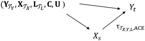The crucial issue is that they are not affected by the exposure $X_s,$ and act as a mediator on the pathway from $X_s$ to $Y_t.$ In research practice, this is often achieved by measuring the time-varying covariates and the prior values of the outcome not after the exposure, that is $t_k^{(L)}\le s$ and $t_k^{(Y)}\le s.$ The relationship between the covariates, the exposure, and the outcome is depicted in Figure 1, where ${\mathrm{\tau }}_{{\mathcal{T}}_{X,Y,L},\mathrm{ACE}}$ denotes the average causal effect (ACE) of $X_s$ on $Y_t.$

Figure 1. Causal diagram that shows the relationship between the covariates, the exposure $X_s,$ and the outcome $Y_t.$ ${\mathrm{\tau }}_{{\mathcal{T}}_{X,Y,L},\mathrm{ACE}}$ denotes the average causal effect (ACE) of $X_s$ on $Y_t.$

We now consider the causal effect function ${\mathrm{\tau }}_{{\mathcal{T}}_{X,Y,L}}\left(x\right)=\mathrm{E}\left(Y_t\left(x\right)\right),$ the expectation of the potential outcomes $Y_t\left(x\right)$ if $X_s$ would be fixed to $x.$ The goal is to estimate the causal effect function ${\mathrm{\tau }}_{{\mathcal{T}}_{X,Y,L}}\left(x\right)$ from the data ($Y_t,$ $X_s,$ ${\mathbf{Y}}_{{\mathcal{T}}_Y},{\mathbf{X}}_{{\mathcal{T}}_X},{\mathbf{L}}_{{\mathcal{T}}_L},\mathbf{C},\mathbf{U}$). To simplify notation, we set $\mathbf{W}=({\mathbf{Y}}_{{\mathcal{T}}_Y},{\mathbf{X}}_{{\mathcal{T}}_X},{\mathbf{L}}_{{\mathcal{T}}_L},\mathbf{C},\mathbf{U}$). If the ignorability assumption holds, the conditional expectation function can be identified as follows: (2) $${\mathrm{\tau }}_{{\mathcal{T}}_{X,Y,L}}\left(x\right)=\mathrm{E}\left[Y_t\left(x\right)\right]=\int \mathrm{E}\left(Y_t\right|X_s=x,\mathbf{W}=\mathbf{w}\left)f_{\mathbf{W}}\right(\mathbf{w})d\mathbf{w},$$(2) where $f_{\mathbf{W}}$ denotes the joint density of $\mathbf{W}.$ In other words, the expected values of the potential outcomes can be determined by averaging the conditional expectation of the outcome given the covariates and the exposure level across the covariate distribution.

In general, the causal effect function ${\mathrm{\tau }}_{{\mathcal{T}}_{X,Y,L}}$ can be nonlinear. In order to quantify an average causal effect by a weighted average slope, we assume that the conditional expectation function ${\mathrm{\tau }}_{{\mathcal{T}}_{X,Y,L}}$ is modeled as a linear function of the exposure values $x$ at time $s,$ where the approximation is weighted according to the density of $X_s$: (3) $${\mathrm{\tau }}_{{\mathcal{T}}_{X,Y,L}}\left(x\right)\simeq \mathrm{\alpha }+{\mathrm{\tau }}_{{\mathcal{T}}_{X,Y,L},\mathrm{ACE}}x,$$(3) where the parameter ${\mathrm{\tau }}_{{\mathcal{T}}_{X,Y,L},\mathrm{ACE}}$ denotes the average causal effect (ACE). The ACE can be interpreted as a weighted average slope by increasing the exposure level by one unit from $x$ to $x+1.$ The linear best approximation in Equation (3)(3) $${\mathrm{\tau }}_{{\mathcal{T}}_{X,Y,L}}\left(x\right)\simeq \mathrm{\alpha }+{\mathrm{\tau }}_{{\mathcal{T}}_{X,Y,L},\mathrm{ACE}}x,$$(3) is provided by the least-squares estimate ${\mathrm{\tau }}_{{\mathcal{T}}_{X,Y,L},\mathrm{ACE}}$ (4) $${\mathrm{\tau }}_{{\mathcal{T}}_{X,Y,L},\mathrm{ACE}}=\frac{\int \left({\mathrm{\tau }}_{{\mathcal{T}}_{X,Y,L}}\right(x)-{\mathrm{\tau }}_t)(x-{\mathrm{\mu }}_{X_s})f_{X_s}\left(x\right)\mathrm{d}x}{\mathrm{Var}\left(X_s\right)},$$(4) where ${\mathrm{\tau }}_t=\int {\mathrm{\tau }}_{{\mathcal{T}}_{X,Y,L}}\left(x\right)f_{X_s}(x)\mathrm{d}x$ is the expected value of the potential outcomes, and $f_{X_s}$ denotes the density function of $X_s.$ The parameter ${\mathrm{\tau }}_{{\mathcal{T}}_{X,Y,L},\mathrm{ACE}}$ can be interpreted as a weighted average slope across all slopes and is the linear best approximation to the true regression function (Angrist & Pischke, 2009; Berk et al., 2014). Equation (3)(3) $${\mathrm{\tau }}_{{\mathcal{T}}_{X,Y,L}}\left(x\right)\simeq \mathrm{\alpha }+{\mathrm{\tau }}_{{\mathcal{T}}_{X,Y,L},\mathrm{ACE}}x,$$(3) is also known as a marginal structural model (MSM), which specifies a model for the marginal mean of the potential outcomes as a function of the exposure, in which the effects of confounding variables have been removed (Daniel et al., 2013; Hernán & Robins, 2020).

We now show that a conventional linear regression model can be used to obtain an unbiased estimate of the causal effect ${\mathrm{\tau }}_{{\mathcal{T}}_{X,Y,L},\mathrm{ACE}}$ when all relevant covariates of the ignorability assumption are included (Keogh et al., 2018). To this end, we assume that all covariates are linearly related to the outcome. The outcome $Y_t$ is then given as follows (5) $$Y_t={\mathrm{\gamma }}_{Y_t}{+ {\mathrm{\gamma }}_{Y_t{X}_s}\hspace{0.17em}{X}_s+{\mathbf{\gamma }}^{\mathit{\prime }}\mathbf{W}+\mathrm{\epsilon }}_{Y_t}.$$(5)

It can now be shown that the coefficient ${\mathrm{\gamma }}_{Y_t{X}_s}$ provides the average causal effect ${\mathrm{\tau }}_{{\mathcal{T}}_{X,Y,L},\mathrm{ACE}}.$ Using the relationship in Equation (5)(5) $$Y_t={\mathrm{\gamma }}_{Y_t}{+ {\mathrm{\gamma }}_{Y_t{X}_s}\hspace{0.17em}{X}_s+{\mathbf{\gamma }}^{\mathit{\prime }}\mathbf{W}+\mathrm{\epsilon }}_{Y_t}.$$(5) , we derive with Equation (2)(2) $${\mathrm{\tau }}_{{\mathcal{T}}_{X,Y,L}}\left(x\right)=\mathrm{E}\left[Y_t\left(x\right)\right]=\int \mathrm{E}\left(Y_t\right|X_s=x,\mathbf{W}=\mathbf{w}\left)f_{\mathbf{W}}\right(\mathbf{w})d\mathbf{w},$$(2) (6) $${\mathrm{\tau }}_{{\mathcal{T}}_{X,Y,L}}\left(x\right)=\int [{\mathrm{\gamma }}_{Y_t}+{\mathrm{\gamma }}_{Y_t{X}_s}\hspace{0.17em}x+{\mathbf{\gamma }}^{\mathit{\prime }}\mathbf{w}]f_{\mathbf{W}}\left(\mathbf{w}\right)\mathrm{d}\mathbf{w}=\mathrm{\alpha }+{\mathrm{\gamma }}_{Y_t{X}_s}\hspace{0.17em}x,$$(6) where $\mathrm{\alpha }={\mathrm{\gamma }}_{Y_t}+{\mathbf{\gamma }}^{\mathit{\prime }}\mathrm{E}(\mathbf{W}$). The conditional expectation function strictly follows a linear form, and we, therefore, obtain the identity ${\mathrm{\tau }}_{{\mathcal{T}}_{X,Y,L},\mathrm{ACE}}={\mathrm{\gamma }}_{Y_t{X}_s}$ by comparing (6) with the specification (3). Thus, the regression coefficient ${\mathrm{\gamma }}_{Y_t{X}_s}$ of a standard regression analysis provides an unbiased estimate of the causal effect ${\mathrm{\tau }}_{{\mathcal{T}}_{X,Y,L},\mathrm{ACE}}$ when all relevant covariates (i.e., $\mathbf{W}=({\mathbf{Y}}_{{\mathcal{T}}_Y},{\mathbf{X}}_{{\mathcal{T}}_X},{\mathbf{L}}_{{\mathcal{T}}_L},\mathbf{C},\mathbf{U}$)) are included.

It should be emphasized that ignorability is a strong assumption that should not be taken lightly.¹ In practical applications, the ignorability assumption implies that all relevant covariates (needed to fulfill the ignorability assumption in Equation (1)(1) $$Y_t\left(x\right) \perp X_s | {\mathbf{Y}}_{{\mathcal{T}}_Y},{\mathbf{X}}_{{\mathcal{T}}_X},{\mathbf{L}}_{{\mathcal{T}}_L},\mathbf{C},\mathbf{U} \text{for all }x\in {\mathcal{X}}_{X_s},$$(1) ) are observed. It is vital that this aspect of the ignorability assumption cannot be empirically tested and needs to be justified by substantive knowledge (Aronow & Miller, 2019). However, in the presence of unmeasured confounders (e.g., $\mathbf{U}$ is not included in Equation (5)(5) $$Y_t={\mathrm{\gamma }}_{Y_t}{+ {\mathrm{\gamma }}_{Y_t{X}_s}\hspace{0.17em}{X}_s+{\mathbf{\gamma }}^{\mathit{\prime }}\mathbf{W}+\mathrm{\epsilon }}_{Y_t}.$$(5) ), the coefficient ${\mathrm{\gamma }}_{Y_t{X}_s}$ from Equation (5)(5) $$Y_t={\mathrm{\gamma }}_{Y_t}{+ {\mathrm{\gamma }}_{Y_t{X}_s}\hspace{0.17em}{X}_s+{\mathbf{\gamma }}^{\mathit{\prime }}\mathbf{W}+\mathrm{\epsilon }}_{Y_t}.$$(5) provides a biased estimate of ${\mathrm{\tau }}_{{\mathcal{T}}_{X,Y,L},\mathrm{ACE}}.$

1.2. Specification Issues

Even if all relevant covariates are measured and included in the regression, it is crucial that the relationship between the covariates $\mathbf{W}$ and the outcome $Y_t$ is correctly specified in a given application. More specifically, this requires that the functional form of the relationship is correctly specified in the analysis models (e.g., squared terms of predictors are included if quadratic effects exist). Powerful machine learning methods allow for very flexible estimation of functional relationships (Athey & Imbens, 2019; van der Laan & Rose, 2018). It should also be emphasized that no assumptions about the distribution of covariates $\mathbf{W}$ are included in the definition of the causal effect. In particular, there are no assumptions about the process $(X_t,{\mathbf{L}}_t,Y_t),$ and the fact that the cross-lagged effect can be obtained from a conventional regression model makes evident that there is no need for modeling the process in $X_t,$ ${\mathbf{L}}_t,$ or $Y_t.$ However, modeling the process might be advantageous for identifying the effects of time-invariant unobserved confounders $\mathbf{U}$ when estimating the cross-lagged effect. To sum up, it is vital to distinguish the definition of a causal effect from modeling a process $(X_t,{\mathbf{L}}_t,Y_t).$ The structural parameter in a well-fitting model for the process $(X_t,{\mathbf{L}}_t,Y_t)$ can be wholly unrelated to the causal effect of interest.

2. Estimating a Cross-Lagged Effect: Controlling for Measured Confounding

In the following, we discuss different models that have been proposed for estimating cross-lagged effects. We start with models that assume no unmeasured confounding and assume a longitudinal panel design in which two variables $Y_t$ and $X_t$ and a p × 1 vector of time-varying covariates ${\mathbf{L}}_t$ are repeatedly measured at equally spaced intervals across time $t$ ($t=1,\dots ,T$). The time-varying variables are combined in the (p + 2)×1 vector ${\mathbf{Z}}_t=(X_t, Y_t, {\mathbf{L}}_t).$ In addition, we consider a k × 1 vector $\mathbf{C}$ of covariates that are constant across the investigated time period. For simplicity, we further assume that the variables are mean-centered at each wave. The main focus is on estimating the causal effect of $X_{t-1}$ on $Y_t.$

2.1. Cross-Lagged Panel Model with Lag-1 Effects (CL1)

The CLPM (Finkel, 1995; Kessler & Greenberg, 1981; Little, 2013) with lag-1 effects and covariates is given by (7) $${\mathbf{Z}}_t={{\mathbf{B}}_{t,t-1}\mathbf{Z}}_{t-1}+{\mathbf{\Gamma }}_t\mathbf{C}+{\mathbf{e}}_t \text{ for }t\ge 2,$$(7) where ${\mathbf{B}}_{t,t-1}$ is a ($p+2)\times (p+2)$ matrix of regression coefficients, including the autoregressive and cross-lagged parameters. The ($p+2)\times k$ matrix ${\mathbf{\Gamma }}_t$ represents the (potentially) time-varying effects of the time-invariant covariates. The ($p+2)\times 1$ vector of residuals ${\mathbf{e}}_t$ denotes correlated random components that are unrelated to previous time points and normally distributed with zero means.

The CLPM can be estimated with only two waves of data. With more than two waves, the autoregressive and cross-lagged parameters can be constrained to be invariant across waves, that is ${\mathbf{B}\equiv \mathbf{B}}_{t,t-1}$ for $t\ge 2.$ This can be reasonable if the time intervals between the waves have a similar length (Little, 2013). Moreover, a constrained estimate can be interpreted as an average of the two causal effects from $t-2$ to $t-1$ and from $t-1$ to $t.$

If the main interest is in estimating the effect of $X_{t-1}$ on $Y_t,$ the cross-lagged panel model with freely estimated parameters is equivalent to estimating a single regression with $Y_t$ as the outcome variable. In the bivariate case (i.e., ${\mathbf{Z}}_t=(X_t,Y_t)$) without covariates, the regression is given by (8) $$Y_t={\mathrm{\beta }}_{Y_t{Y}_{t-1}}{Y}_{t-1}+{\mathrm{\beta }}_{Y_t{X}_{t-1}}{X}_{t-1}+e_{Y_t}$$(8)

Thus, the CLPM controls for preexisting differences in the outcome when assessing the effect of the exposure and is a special case of a more general class of conditioning methods in which an estimate of the causal effect is obtained by conditioning on the pretest and other observed covariates (see VanderWeele et al., 2016). It should be emphasized that the regression model in Equation (8)(8) $$Y_t={\mathrm{\beta }}_{Y_t{Y}_{t-1}}{Y}_{t-1}+{\mathrm{\beta }}_{Y_t{X}_{t-1}}{X}_{t-1}+e_{Y_t}$$(8) includes one of the most basic and frequently used analysis strategies in psychology (Orth et al., 2021).

As the traditional CLPM only considers the effects of the previous measurement wave (i.e., lag-1 effects), we will refer to the model as CL1. The CL1 for T = 3 is depicted as a path diagram in the left panel of Figure 2. It needs to be emphasized that recent discussion of the CLPM (e.g., Bailey et al., 2020; Dietvorst et al., 2018; Littlefield et al., 2021; Lucas, 2022; Usami, Murayama, et al., 2019) mainly focused on the CL1 and did not consider the role of higher-order lags (e.g., lag-2 effects).

Figure 2. Path diagrams of the cross-lagged panel models with lag-1 (CL1) and lag-2 (CL2) effects for three measurement waves.

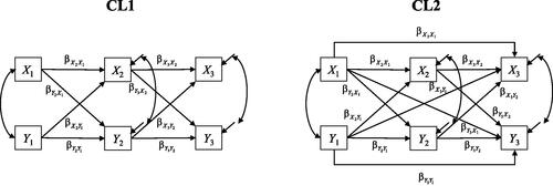
2.2. Cross-Lagged Panel Model with Lag-2 Effects (CL2)

The CL1 in Equation (7)(7) $${\mathbf{Z}}_t={{\mathbf{B}}_{t,t-1}\mathbf{Z}}_{t-1}+{\mathbf{\Gamma }}_t\mathbf{C}+{\mathbf{e}}_t \text{ for }t\ge 2,$$(7) can be extended to a CL2 that includes the effects of variables from two previous time points (i.e., lag-2 effects): (9) $${\mathbf{Z}}_t={{\mathbf{B}}_{t,t-1}\mathbf{Z}}_{t-1}+{{\mathbf{B}}_{t,t-2}\mathbf{Z}}_{t-2}+{\mathbf{\Gamma }}_t\mathbf{C}+{\mathbf{e}}_t \text{ for }t\ge 2,$$(9) where ${\mathbf{B}}_{t,t-2}$ denotes a ($p+2)\times (p+2)$ matrix of regression coefficients that includes the stability effects (e.g., the extent to which $X_t$ depends on $X_{t-2}$ over and above the effect of $X_{t-1};$ second-order autoregression), and the lag-2 cross-lagged effects. The CL1 is a CL2 with only lag-1 effects and is thus nested within the CL2.

There are different perspectives on the importance of including these lag-2 effects in the CL2 (Little, 2013). One view is that they consider delayed effects that are not captured by the lag-1 effects (e.g., Asendorpf, 2021; Marsh et al., 2018). However, it has been argued that it is often difficult to justify which psychological mechanism could be responsible for these delayed effects and that direct effects (i.e., lag-1 effects) are often more plausible (e.g., Ehm et al., 2019). From a causal inference perspective, the main motivation for including lag-2 effects is a more comprehensive control for confounding. VanderWeele (2021, p. 607) argues that if prior exposure $X_{t-2}$ affects subsequent exposure $X_{t-1},$ and also independently affects the outcome $Y_t$ not through $X_{t-1}$ then prior exposure itself confounds the cross-lagged of $X_{t-1}$ on $Y_t.$ Thus, prior values of the exposure and outcome measures ($X_{t-2}$ and $Y_{t-2}$) can be considered covariates that allow for stronger control of confounding. In some applications, it may even be necessary to control for lag-3 effects of lagged exposures ($X_{t-3})$ and outcomes ($Y_{t-3}).$ VanderWeele et al. (2020) provide a detailed discussion of the benefits of controlling for the history of previous exposure and outcome variables.

In the bivariate case, estimating a cross-lagged effect with a CL2 is equivalent to a single regression equation in which the outcome is regressed on the exposure $X_{t-1}$ and the other variables (10) $$Y_t={\mathrm{\beta }}_{Y_t{Y}_{t-1}}{Y}_{t-1}+{\mathrm{\beta }}_{Y_t{Y}_{t-2}}{Y}_{t-2}{+\mathrm{ }\mathrm{\beta }}_{Y_t{X}_{t-1}}{X}_{t-1}{+\mathrm{ }\mathrm{\beta }}_{Y_t{X}_{t-2}}{X}_{t-2}{+\mathrm{ }e}_{Y_t}$$(10) where ${\mathrm{\beta }}_{Y_t{X}_{t-1}}$ denotes the cross-lagged effect of interest. However, like the CL1, the CL2 will produce biased estimates of the cross-lagged effect if unmeasured confounders $\mathbf{U}$ exist that are part of the ignorability assumption (see Equation (1)(1) $$Y_t\left(x\right) \perp X_s | {\mathbf{Y}}_{{\mathcal{T}}_Y},{\mathbf{X}}_{{\mathcal{T}}_X},{\mathbf{L}}_{{\mathcal{T}}_L},\mathbf{C},\mathbf{U} \text{for all }x\in {\mathcal{X}}_{X_s},$$(1) ) but not included in Equation (10)(10) $$Y_t={\mathrm{\beta }}_{Y_t{Y}_{t-1}}{Y}_{t-1}+{\mathrm{\beta }}_{Y_t{Y}_{t-2}}{Y}_{t-2}{+\mathrm{ }\mathrm{\beta }}_{Y_t{X}_{t-1}}{X}_{t-1}{+\mathrm{ }\mathrm{\beta }}_{Y_t{X}_{t-2}}{X}_{t-2}{+\mathrm{ }e}_{Y_t}$$(10) .

3. Estimating a Cross-Lagged Effect: Controlling for Unmeasured Confounding

One advantage of longitudinal data is that they offer the potential to control for the effects of unmeasured confounder variables when estimating causal effects. In the following, we discuss three different strategies that have been suggested for estimating cross-lagged effects in the presence of unmeasured time-invariant confounders $\mathbf{U}.$ The basic idea of these approaches is to use parametric modeling assumptions to identify additional latent variables that adjust for the effects of the unmeasured confounders.

3.1. Observation-Level Approaches

In the observation-level approach, the effects of unmeasured confounders are taken into account by including additional latent variables in the CL1 model (see Equation (7)(7) $${\mathbf{Z}}_t={{\mathbf{B}}_{t,t-1}\mathbf{Z}}_{t-1}+{\mathbf{\Gamma }}_t\mathbf{C}+{\mathbf{e}}_t \text{ for }t\ge 2,$$(7) ): (11) $${\mathbf{Z}}_t={{\mathbf{B}}_{t,t-1}\mathbf{Z}}_{t-1}+{\mathbf{\Gamma }}_t\mathbf{C}+{\mathbf{\Lambda }}_t\mathbf{U}+{\mathbf{e}}_t \mathrm{for} t\ge 2,$$(11) where ${\mathbf{Z}}_t,$ and $\mathbf{C}$ are defined as above, and $\mathbf{U}$ is a $q\times 1$ vector of latent variables with a ($p+2)\times q$ loading matrix ${\mathbf{\Lambda }}_t$ (Bollen & Brand, 2010). The latent variables $\mathbf{U}$ are referred to as unit effects, unobserved effects, or individual effects in the literature (Andersen, 2021; Hsiao, 2014; Wooldridge, 2010; Zyphur et al., 2020) and are supposed to capture the effects of unmeasured time-invariant variables. The latent variables can be identified by setting the variances of the latent variables to one. The loadings ${\mathbf{\Lambda }}_t$ represent the—potentially time-varying—effects of $\mathbf{U}$ on the observed variables. In many applications, ${\mathbf{\Lambda }}_t$ is assumed to be diagonal (i.e., ${\mathbf{Z}}_t$ and $\mathbf{U}$ have the same dimension), and the loadings are fixed to represent individual differences in level and growth (e.g., linear trends) in the observed variables ${\mathbf{Z}}_t$ (Bollen & Curran, 2004; Usami, Murayama, et al., 2019). However, more exploratory approaches have been proposed, particularly in the econometrics literature, in which ${\mathbf{\Lambda }}_t$ is not diagonal and the dimension of $\mathbf{U}$ is not assumed to be known (e.g., Bai & Li, 2014; De Vos & Everaert, 2021). have Furthermore, the time-invariant covariates $\mathbf{C}$ are assumed to be uncorrelated with the latent factors $\mathbf{U},$ that is $\mathrm{Cov}\left(\mathbf{C},\mathbf{U}\right)=0.$ This restriction is necessary for identifying the model (e.g., Allison et al., 2017; Bollen & Brand, 2010). The latent variables in $\mathbf{U}$ have also been characterized as accumulating factors (Usami, 2021; Usami, Murayama et al., 2019).

At the first wave (t = 1), the vector of variables ${\mathbf{Z}}_1$ are treated as exogeneous (i.e., predetermined; Bollen & Brand, 2010) and are correlated with the time-invariant covariates $\mathbf{C},$ and the latent variables $\mathbf{U}$ (12) $$\mathrm{Cov}\left({\mathbf{Z}}_1,\mathbf{C}\right)={\mathbf{\Psi }}_{{\mathbf{Z}}_1\mathbf{C}} \text{and Cov}\left({\mathbf{Z}}_1,\mathbf{U}\right)={\mathbf{\Psi }}_{{\mathbf{Z}}_1\mathbf{U}}$$(12) where ${\mathbf{\Psi }}_{{\mathbf{Z}}_1\mathbf{C}}$ and ${\mathbf{\Psi }}_{{\mathbf{Z}}_1\mathbf{U}}$ denote ($p+2)\times k$ and ($p+2)\times q$ covariance matrices in which all unique elements are freely estimated. An alternative representation of the covariances at $t=1$ was recently suggested by Zyphur et al. (2020) (13) $${\mathbf{Z}}_1={\mathbf{\Gamma }}_1\mathbf{C}+{\mathbf{\Lambda }}_1\mathbf{U}+{\mathbf{e}}_1$$(13)

In this specification, the loadings in ${\mathbf{\Lambda }}_1$ are freely estimated to represent the covariance of ${\mathbf{Z}}_1$ and $\mathbf{U}.$

One crucial aspect of the model in Equations (11)(11) $${\mathbf{Z}}_t={{\mathbf{B}}_{t,t-1}\mathbf{Z}}_{t-1}+{\mathbf{\Gamma }}_t\mathbf{C}+{\mathbf{\Lambda }}_t\mathbf{U}+{\mathbf{e}}_t \mathrm{for} t\ge 2,$$(11) and (12)(12) $$\mathrm{Cov}\left({\mathbf{Z}}_1,\mathbf{C}\right)={\mathbf{\Psi }}_{{\mathbf{Z}}_1\mathbf{C}} \text{and Cov}\left({\mathbf{Z}}_1,\mathbf{U}\right)={\mathbf{\Psi }}_{{\mathbf{Z}}_1\mathbf{U}}$$(12) (or (11) and (13)) is the identification of all model parameters, which has to be established on a model-by-model basis (e.g., Bollen & Curran, 2004). It should be mentioned that with a large number of waves, the model can also include higher-order lags (e.g., lag-2 effects) for the time-varying variables. However, most applications are restricted to AR(1) processes (i.e., lag-1 effects). In the following, we discuss four different observation-level models that have been proposed for estimating cross-lagged effects in the presence of unmeasured confounders. We restrict our discussion to the bivariate case without additional covariates.

3.1.1. Unidimensional Latent Factor Model (OL1)

Finkel (1995) proposed an observation-level model with a single latent factor. This model is identified if at least three measurement waves are available, and the regression coefficients are assumed to be invariant across time. This model is given as follows: (14) $$\underset{{\mathbf{Z}}_t}{\underbrace{\left(\genfrac{}{}{0pt}{}{X_t}{Y_t}\right)}}=\underset{{\mathbf{B}}_{t,t-1}}{\underbrace{\left(\genfrac{}{}{0pt}{}{{\mathrm{\beta }}_{X_t{X}_{t-1}}}{{\mathrm{\beta }}_{Y_t{X}_{t-1}}}\genfrac{}{}{0pt}{}{{\mathrm{\beta }}_{X_t{Y}_{t-1}}}{{\mathrm{\beta }}_{Y_t{Y}_{t-1}}}\right)}}\underset{{\mathbf{Z}}_{t-1} }{\underbrace{\left(\genfrac{}{}{0pt}{}{X_{t-1}}{Y_{t-1}}\right)}}+\underset{{\mathbf{\Lambda }}_t}{\underbrace{\left(\genfrac{}{}{0pt}{}{{\mathrm{\lambda }}_{X_t,U_1}}{{\mathrm{\lambda }}_{Y_t,U_1}}\right)}}\underset{\mathbf{U}}{\underbrace{U_1}}+\underset{{\mathbf{e}}_t}{\underbrace{\left(\genfrac{}{}{0pt}{}{e_{X_t}}{e_{Y_t}}\right)}} \mathrm{f}\mathrm{or} t\ge 2,$$(14)

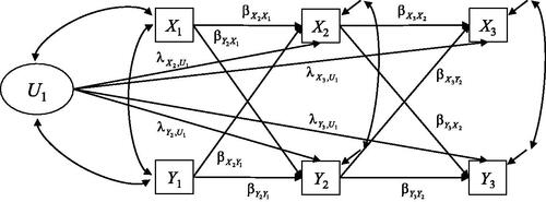
where the regression coefficients are set equal across time, that is ${\mathbf{B}\equiv \mathbf{B}}_{t,t-1}$ for $t\ge 2.$ At $t=1,$ $X_1$ and $Y_1$ are allowed to covary with $U_1.$ The path diagram of the model is depicted for T = 3 in Figure 3. The latent variable $U_1$ can be interpreted as an unmeasured confounder that affects the variables $X_t$ and $Y_t,$ and distorts the estimation of the cross-lagged effect in a CL1. Note that $U_1$ is assumed to be time-invariant, but the effects in ${\mathbf{\Lambda }}_t$ are allowed to vary across time. We refer to the model in Equation (14)(14) $$\underset{{\mathbf{Z}}_t}{\underbrace{\left(\genfrac{}{}{0pt}{}{X_t}{Y_t}\right)}}=\underset{{\mathbf{B}}_{t,t-1}}{\underbrace{\left(\genfrac{}{}{0pt}{}{{\mathrm{\beta }}_{X_t{X}_{t-1}}}{{\mathrm{\beta }}_{Y_t{X}_{t-1}}}\genfrac{}{}{0pt}{}{{\mathrm{\beta }}_{X_t{Y}_{t-1}}}{{\mathrm{\beta }}_{Y_t{Y}_{t-1}}}\right)}}\underset{{\mathbf{Z}}_{t-1} }{\underbrace{\left(\genfrac{}{}{0pt}{}{X_{t-1}}{Y_{t-1}}\right)}}+\underset{{\mathbf{\Lambda }}_t}{\underbrace{\left(\genfrac{}{}{0pt}{}{{\mathrm{\lambda }}_{X_t,U_1}}{{\mathrm{\lambda }}_{Y_t,U_1}}\right)}}\underset{\mathbf{U}}{\underbrace{U_1}}+\underset{{\mathbf{e}}_t}{\underbrace{\left(\genfrac{}{}{0pt}{}{e_{X_t}}{e_{Y_t}}\right)}} \mathrm{f}\mathrm{or} t\ge 2,$$(14) as OL1. It should be emphasized that $U_1$ is not actually measured but that the effects of the confounder $U_1$ are identified by parametric modelling assumptions. Finkel (1995, p. 83) refers to $U_1$ as a “phantom variable” that can be used to test for spurious associations.

Figure 3. Path diagram of an observation-level model with a single latent variable (OL1; Finkel, 1995) for three measurement waves.

3.1.2. Twodimensional Latent Factor Model (OL2)

Another variant of the observational-level approach has been proposed by Dishop and DeShon (2021; see also Bollen & Brand, 2010). In this specification, the number of additional latent variables in $\mathbf{U}$ corresponds to the number of time-varying variables in ${\mathbf{Z}}_t$

(15) $$\left(\begin{array}{c}{X}_t\\ Y_t\end{array}\right)=\left(\begin{array}{cc}{\mathrm{\beta }}_{X_t{X}_{t-1}}& {\mathrm{\beta }}_{X_t{Y}_{t-1}}\\ {\mathrm{\beta }}_{Y_t{X}_{t-1}}& {\mathrm{\beta }}_{Y_t{Y}_{t-1}}\end{array}\right)\left(\begin{array}{c}{X}_{t-1}\\ Y_{t-1}\end{array}\right)+\left(\begin{array}{cc}{\mathrm{\lambda }}_{X_t,U_1}& 0\\ 0& {\mathrm{\lambda }}_{Y_t,U_2}\end{array}\right)\left(\begin{array}{c}{U}_1\\ U_2\end{array}\right)+\left(\begin{array}{c}{e}_{X_t}\\ e_{Y_t}\end{array}\right) \mathrm{f}\mathrm{or} t\ge 2,$$(15) where the diagonal loading matrices ${\mathbf{\Lambda }}_t\equiv \mathbf{\Lambda },$ and regression coefficients ${\mathbf{B}\equiv \mathbf{B}}_{t,t-1}$ are set equal across time for $t\ge 2.$ The latent variables $U_1$ and $U_2$ are assumed to be correlated. 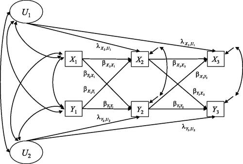At $t=1,$ the two observed variables $X_1$ and $Y_1$ are allowed to be freely correlated with the latent variables (see Equation (12)(12) $$\mathrm{Cov}\left({\mathbf{Z}}_1,\mathbf{C}\right)={\mathbf{\Psi }}_{{\mathbf{Z}}_1\mathbf{C}} \text{and Cov}\left({\mathbf{Z}}_1,\mathbf{U}\right)={\mathbf{\Psi }}_{{\mathbf{Z}}_1\mathbf{U}}$$(12) ) Again, this guarantees that $X_1$ and $Y_1$ are treated as exogeneous (i.e., predetermined). The path diagram of this model is shown for $T=3$ in Figure 4. Note that the restriction of equal effects of the latent variables in $\mathbf{U}$ can be removed by freely estimating the loadings in ${\mathbf{\Lambda }}_t$ (see Dishop & DeShon, 2021, p. 17). Furthermore, it would be possible to specify ${\mathbf{\Lambda }}_t$ to be nondiagonal (i.e., cross loadings), and allow for effects of $U_1$ on $Y_t,$ and $U_2$ on $X_t.$ In the following, we refer to the model in Equation (15)(15) $$\left(\begin{array}{c}{X}_t\\ Y_t\end{array}\right)=\left(\begin{array}{cc}{\mathrm{\beta }}_{X_t{X}_{t-1}}& {\mathrm{\beta }}_{X_t{Y}_{t-1}}\\ {\mathrm{\beta }}_{Y_t{X}_{t-1}}& {\mathrm{\beta }}_{Y_t{Y}_{t-1}}\end{array}\right)\left(\begin{array}{c}{X}_{t-1}\\ Y_{t-1}\end{array}\right)+\left(\begin{array}{cc}{\mathrm{\lambda }}_{X_t,U_1}& 0\\ 0& {\mathrm{\lambda }}_{Y_t,U_2}\end{array}\right)\left(\begin{array}{c}{U}_1\\ U_2\end{array}\right)+\left(\begin{array}{c}{e}_{X_t}\\ e_{Y_t}\end{array}\right) \mathrm{f}\mathrm{or} t\ge 2,$$(15) as OL2.

Figure 4. Path diagram of an observation-level model with two latent variables (OL2; Dishop & DeShon, 2021; see also Bollen & Brand, 2010) for three measurement waves.

3.1.3. Twodimensional Latent Factor Model with Loadings at Time 1 (OL3 and OL4)

A slightly different version of an observation-level model with two latent variables has been discussed by Zyphur et al. (2020; see also Shamsollahi et al., 2021). They used the specification in Equation (13)(13) $${\mathbf{Z}}_1={\mathbf{\Gamma }}_1\mathbf{C}+{\mathbf{\Lambda }}_1\mathbf{U}+{\mathbf{e}}_1$$(13) to represent the associations between ${\mathbf{Z}}_1$ and $\mathbf{U}$ (16) $$\left(\genfrac{}{}{0pt}{}{X_1}{Y_1}\right)=\left(\begin{array}{cc}{\lambda }_{X_1,U_1}& 0\\ 0& {\lambda }_{Y_1,U_2}\end{array}\right)\left(\genfrac{}{}{0pt}{}{U_1}{U_2}\right)+\left(\genfrac{}{}{0pt}{}{e_{X_1}}{e_{Y_1}}\right),$$(16) where ${\mathbf{\Lambda }}_1$ is assumed to be diagonal, and only ${\mathrm{\lambda }}_{X_1,U_1}$ and ${\mathrm{\lambda }}_{Y_1,U_2}$ are estimated (the cross-loadings are set to zero, i.e., ${\mathrm{\lambda }}_{X_1,U_2}={\mathrm{\lambda }}_{Y_1,U_1}=0$). For $t\ge 2,$ the model discussed in Zyphur et al. (2020) is given by Equation (15)(15) $$\left(\begin{array}{c}{X}_t\\ Y_t\end{array}\right)=\left(\begin{array}{cc}{\mathrm{\beta }}_{X_t{X}_{t-1}}& {\mathrm{\beta }}_{X_t{Y}_{t-1}}\\ {\mathrm{\beta }}_{Y_t{X}_{t-1}}& {\mathrm{\beta }}_{Y_t{Y}_{t-1}}\end{array}\right)\left(\begin{array}{c}{X}_{t-1}\\ Y_{t-1}\end{array}\right)+\left(\begin{array}{cc}{\mathrm{\lambda }}_{X_t,U_1}& 0\\ 0& {\mathrm{\lambda }}_{Y_t,U_2}\end{array}\right)\left(\begin{array}{c}{U}_1\\ U_2\end{array}\right)+\left(\begin{array}{c}{e}_{X_t}\\ e_{Y_t}\end{array}\right) \mathrm{f}\mathrm{or} t\ge 2,$$(15) . In the following, we refer to this model as OL3.

Zyphur et al. (2020) also discuss the possibility to freely estimate the loadings in the diagonal matrices ${\mathbf{\Lambda }}_t$ (for $t\ge 2$). As mentioned before, this would allow the latent variables $U_1$ and $U_2$ to have time-varying effects (see also Bollen & Brand, 2010, Allison et al., 2017). We refer to this model as OL4. The four observation-level models, which are also included in the simulation studies, are summarized in Table 1.

Table 1. Overview of different latent variable-type models that adjust for effects of unmeasured variables $\mathbf{U}.$

		Effects of $\mathbf{U}$
Model	Dimension $\mathbf{U}$	Time 1	Time 2 and 3	Coefficients
Observation-Level
OL1	1	$\mathrm{Cov}\left({\mathbf{Z}}_1,\mathbf{U}\right)={\mathbf{\Psi }}_{{\mathbf{Z}}_1\mathbf{U}}$	${\mathbf{\Lambda }}_2\ne {\mathbf{\Lambda }}_3$	${\mathbf{B}}_{21}={\mathbf{B}}_{32}$
OL2	2	$\mathrm{Cov}\left({\mathbf{Z}}_1,\mathbf{U}\right)={\mathbf{\Psi }}_{{\mathbf{Z}}_1\mathbf{U}}$	${\mathbf{\Lambda }}_2$ and ${\mathbf{\Lambda }}_3$ diagonal; ${\mathbf{\Lambda }}_2={\mathbf{\Lambda }}_3$	${\mathbf{B}}_{21}={\mathbf{B}}_{32}$
OL3	2	${\mathbf{\Lambda }}_1$ diagonal	${\mathbf{\Lambda }}_2$ and ${\mathbf{\Lambda }}_3$ diagonal;${\mathbf{\Lambda }}_2={\mathbf{\Lambda }}_3$	${\mathbf{B}}_{21}={\mathbf{B}}_{32}$
OL4	2	${\mathbf{\Lambda }}_1$ diagonal	${\mathbf{\Lambda }}_2$ and ${\mathbf{\Lambda }}_3$ diagonal; ${\mathbf{\Lambda }}_2\ne {\mathbf{\Lambda }}_3$	${\mathbf{B}}_{21}={\mathbf{B}}_{32}$
Residual-Level
RL1	2	${\mathbf{\Lambda }}_1$ diagonal	${\mathbf{\Lambda }}_2$ and ${\mathbf{\Lambda }}_3$ diagonal; ${\mathbf{\Lambda }}_1={\mathbf{\Lambda }}_2={\mathbf{\Lambda }}_3$	${\mathbf{B}}_{21}={\mathbf{B}}_{32}$
RL2	2	${\mathbf{\Lambda }}_1$ diagonal	${\mathbf{\Lambda }}_2$ and ${\mathbf{\Lambda }}_3$ diagonal;${\mathbf{\Lambda }}_1\ne {\mathbf{\Lambda }}_2\ne {\mathbf{\Lambda }}_3$	${\mathbf{B}}_{21}={\mathbf{B}}_{32}$
RL3	2	${\mathbf{\Lambda }}_1$ diagonal	${\mathbf{\Lambda }}_2$ and ${\mathbf{\Lambda }}_3$ diagonal; ${\mathbf{\Lambda }}_1={\mathbf{\Lambda }}_2={\mathbf{\Lambda }}_3$	${\mathbf{B}}_{21}\ne {\mathbf{B}}_{32}$
Fixed Effects
FED	1	$\mathrm{Cov}\left({\mathbf{Z}}_1,\mathbf{U}\right)={\mathbf{\Psi }}_{{\mathbf{Z}}_1\mathbf{U}}$	${\mathbf{\lambda }}_2={\mathbf{\lambda }}_3$	${\mathbf{\beta }}_{21}={\mathbf{\beta }}_{32}$

Note. OL1 = observation-level model with a single latent factor (Finkel, 1995); OL2 = observation-level model with two latent variables and freely estimated correlations at time 1 (Dishop & DeShon, 2021); OL3 = observation-level model with two latent variables and diagonal loading matrix at time 1 (Zyphur et al., 2020); OL4 = OL3 with non-invariant loadings across time (Zyphur et al., 2020); RL1 = residual-level model with diagonal and time-invariant loading matrices and time-invariant regression coefficients (Hamaker et al., 2015); RL2 = RL1 with non-invariant loading matrices; RL3 = RL1 with freely estimated regression coefficients; FED = fixed effects dynamic panel model (Allison et al., 2017). The variances of the latent variables $\mathbf{U}$ are set to one.

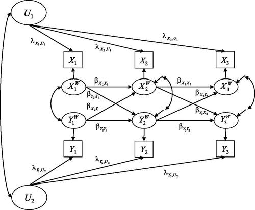
3.2. Residual-Level Approaches

In the residual-level approach, the longitudinal association among the time-varying ${\mathbf{Z}}_t$ are decomposed into a between-person part ${\mathbf{Z}}_t^B$ and occasion-specific within-person deviations ${\mathbf{Z}}_t^W$: (17) $${ \hspace{0.17em}\mathbf{Z}}_t={\mathbf{Z}}_t^B+{\mathbf{Z}}_t^W \text{ for }t=1,\dots ,T$$(17) (18) $${\mathbf{Z}}_t^B={{\mathbf{\Gamma }}_t\mathbf{C}+\mathbf{\Lambda }}_t\mathbf{U} \mathrm{for}\mathrm{ }t=1,\dots ,T$$(18) (19) $${\mathbf{Z}}_1^W={\mathbf{e}}_1 \text{ for }t=1$$(19) (20) $${ \mathbf{Z}}_t^W={{\mathbf{B}}_{t,t-1}\mathbf{Z}}_{t-1}^W+{\mathbf{e}}_t \text{ for }t\ge 2$$(20)

The occasion-specific deviations ${\mathbf{Z}}_t^W$ can be interpreted as residuals that are orthogonal to the between-person part, that is ${\mathbf{Z}}_t^B={{\mathbf{\Gamma }}_t\mathbf{C}+\mathbf{\Lambda }}_t\mathbf{U}$ (see Asparouhov & Muthén, 2021). Thus, the autoregressive and cross-lagged effects (i.e., ${\mathbf{B}}_{t,t-1}$) in Equation (20)(20) $${ \mathbf{Z}}_t^W={{\mathbf{B}}_{t,t-1}\mathbf{Z}}_{t-1}^W+{\mathbf{e}}_t \text{ for }t\ge 2$$(20) are estimated on a residual structure that is purified from the effects of the time-invariant covariates $\mathbf{C}$ and the latent variables $\mathbf{U}.$ At $t=1,$ the occasion-specific deviations are equated with the residuals (see Equation (19)(19) $${\mathbf{Z}}_1^W={\mathbf{e}}_1 \text{ for }t=1$$(19) ). In general, the latent variables $\mathbf{U}$ are allowed to have time-varying effects ${\mathbf{\Lambda }}_t.$ The identification of the latent factor model involving the part ${\mathbf{\Lambda }}_t\mathbf{U}$ needs to be established for each specific application. A particular strength of the residual-level approach is its ability to disaggregate between-person and within-person effects in the analysis of longitudinal data (Curran & Hancock, 2021; Hamaker et al., 2015; Usami et al., 2019).

The main difference between the residual-level and the observation-level approaches is that in the residual-level approach the coefficients are estimated for the decomposed scores ${\mathbf{Z}}_t^W$ instead of the observed scores ${\mathbf{Z}}_t.$ To better compare the two approaches, it is instructive to write Equations (17)(17) $${ \hspace{0.17em}\mathbf{Z}}_t={\mathbf{Z}}_t^B+{\mathbf{Z}}_t^W \text{ for }t=1,\dots ,T$$(17) to (20)(20) $${ \mathbf{Z}}_t^W={{\mathbf{B}}_{t,t-1}\mathbf{Z}}_{t-1}^W+{\mathbf{e}}_t \text{ for }t\ge 2$$(20) for the observed scores (21) $$Z_t=B_{t,t-1}\left(Z_{t-1}-{\Gamma }_{t-1}C-{\Lambda }_{t-1}U\right)+{\Gamma }_{t}C+{\Lambda }_{t}U+e_t =B_{t,t-1}{Z}_{t-1}+\left({\Gamma }_t-B_{t,t-1}{\Gamma }_{t-1}\right)C+\left({\Lambda }_t-B_{t,t-1}{\Lambda }_{t-1}\right)U+e_t \text{ for }t\ge 2$$(21)

The conditions under which the residual-level approach is a re-expression of the observation-level approach (and vice versa) will be further investigated in the section 3.4 “Relationship between the Residual-Level and Observation-Level Approaches”.

3.2.1. Twodimensional Latent Factor Model with Time-Invariant Loadings and Regression Coefficients (RL1)

The most popular residual-level approach is the RI-CLPM (Hamaker et al., 2015) which was introduced to extend the CLPM with lag-1 effects (CL1). In the bivariate case, the RI-CLPM is given by (22) $$\left(\genfrac{}{}{0pt}{}{X_t}{Y_t}\right)=\left(\begin{array}{cc}{\lambda }_{X_t,U_1}& 0\\ 0& {\lambda }_{Y_t,U_2}\end{array}\right)\left(\genfrac{}{}{0pt}{}{U_1}{U_2}\right)+\left(\begin{array}{c}{X}_t^W\\ Y_t^W\end{array}\right)\text{ for }t=1,\dots ,T$$(22) (23) $$\left(\begin{array}{c}{X}_t^W\\ Y_t^W\end{array}\right)=\left(\begin{array}{cc}{\mathrm{\beta }}_{X_t{X}_{t-1}}& {\mathrm{\beta }}_{X_t{Y}_{t-1}}\\ {\mathrm{\beta }}_{Y_t{X}_{t-1}}& {\mathrm{\beta }}_{Y_t{Y}_{t-1}}\end{array}\right)\left(\begin{array}{c}{X}_{t-1}^W\\ Y_{t-1}^W\end{array}\right)+\left(\genfrac{}{}{0pt}{}{e_{X_t}}{e_{Y_t}}\right)\text{ for }t\ge 2$$(23)

The loading matrices ${\mathbf{\Lambda }}_t$ are assumed to be diagonal (e.g., no effects of $U_1$ on $Y_t$), and the loadings ${\lambda }_{X_t,U_1}$ and ${\lambda }_{Y_t,U_2}$ are assumed to be invariant across time (Hamaker et al., 2015). The latent variables $U_1$ and $U_2$ are interpreted as stable trait factors that represent the parts of $X_t$ and $Y_t$ that are completely stable across time. The coefficients ${\mathrm{\beta }}_{X_t{X}_{t-1}}$ and ${\mathrm{\beta }}_{Y_t{Y}_{t-1}}$ represent the autoregressive effects and the coefficients ${\mathrm{\beta }}_{X_t{Y}_{t-1}}$ and ${\mathrm{\beta }}_{Y_t{X}_{t-1}}$ represent the cross-lagged effects. The cross-lagged effects are interpreted as within-person effects. For example, ${\mathrm{\beta }}_{Y_t{X}_{t-1}}$ indicates whether a temporal deviation (i.e., $X_{t-1}^W$) from the stable trait level (i.e., $U_1$) of one construct affects subsequent within-person deviations (i.e., $Y_t^W$) from the stable trait level (i.e., $U_2$) of the other construct. The RI-CLPM is depicted as a path diagram in Figure 5.

Figure 5. Path diagram of the random intercept cross-lagged panel model (RI-CLPM; Hamaker et al., 2015) for three measurement waves.

We also write the RI-CLPM for the observed scores ${\mathbf{Z}}_t$ (see Equation (21)(21) $$Z_t=B_{t,t-1}\left(Z_{t-1}-{\Gamma }_{t-1}C-{\Lambda }_{t-1}U\right)+{\Gamma }_{t}C+{\Lambda }_{t}U+e_t =B_{t,t-1}{Z}_{t-1}+\left({\Gamma }_t-B_{t,t-1}{\Gamma }_{t-1}\right)C+\left({\Lambda }_t-B_{t,t-1}{\Lambda }_{t-1}\right)U+e_t \text{ for }t\ge 2$$(21) ) (24) $$\left(\genfrac{}{}{0pt}{}{X_t}{Y_t}\right)=\left(\begin{array}{cc}{\mathrm{\beta }}_{X_t{X}_{t-1}}& {\mathrm{\beta }}_{X_t{Y}_{t-1}}\\ {\mathrm{\beta }}_{Y_t{X}_{t-1}}& {\mathrm{\beta }}_{Y_t{Y}_{t-1}}\end{array}\right)\left(\begin{array}{c}{X}_{t-1\mathrm{ }}\\ Y_{t-1\mathrm{ }}\end{array}\right)+\left(\begin{array}{cc}{\lambda }_{X_t,U_1}-{\mathrm{\beta }}_{X_t{X}_{t-1}}{\lambda }_{X_{t-1},U_1}& 0\\ 0& {\lambda }_{Y_t,U_2}-{\mathrm{\beta }}_{Y_t{Y}_{t-1}}{\lambda }_{Y_{t-1},U_2}\end{array}\right)\left(\genfrac{}{}{0pt}{}{U_1}{U_2}\right)+\left(\genfrac{}{}{0pt}{}{e_{X_t}}{e_{Y_t}}\right)$$(24)

We refer to the model in Equation (24)(23) $$\left(\begin{array}{c}{X}_t^W\\ Y_t^W\end{array}\right)=\left(\begin{array}{cc}{\mathrm{\beta }}_{X_t{X}_{t-1}}& {\mathrm{\beta }}_{X_t{Y}_{t-1}}\\ {\mathrm{\beta }}_{Y_t{X}_{t-1}}& {\mathrm{\beta }}_{Y_t{Y}_{t-1}}\end{array}\right)\left(\begin{array}{c}{X}_{t-1}^W\\ Y_{t-1}^W\end{array}\right)+\left(\genfrac{}{}{0pt}{}{e_{X_t}}{e_{Y_t}}\right)\text{ for }t\ge 2$$(23) with invariant regression coefficients (i.e., $\mathbf{B}\equiv {\mathbf{B}}_{t,t-1}$) and loadings (i.e., ${\mathbf{\Lambda }\equiv \mathbf{\Lambda }}_t$) across time as RL1.

3.2.2. Twodimensional Latent Factor Model with Time-Varying Loadings or Regression Coefficients (RL2, RL3)

It is also possible to freely estimate the loadings in the diagonal matrices ${\mathbf{\Lambda }}_t.$ This would allow the time-invariant $U_1$ and $U_2$ in Equation (24)(23) $$\left(\begin{array}{c}{X}_t^W\\ Y_t^W\end{array}\right)=\left(\begin{array}{cc}{\mathrm{\beta }}_{X_t{X}_{t-1}}& {\mathrm{\beta }}_{X_t{Y}_{t-1}}\\ {\mathrm{\beta }}_{Y_t{X}_{t-1}}& {\mathrm{\beta }}_{Y_t{Y}_{t-1}}\end{array}\right)\left(\begin{array}{c}{X}_{t-1}^W\\ Y_{t-1}^W\end{array}\right)+\left(\genfrac{}{}{0pt}{}{e_{X_t}}{e_{Y_t}}\right)\text{ for }t\ge 2$$(23) to have time-varying effects. In the following, we refer to this model with freely estimated loadings as RL2. We also consider a model with freely estimated regression coefficients and time-invariant loadings. This model is labeled RL3 and is the original formulation of the RI-CLPM (Hamaker et al., 2015). The three different residual-level models are summarized in Table 1.

3.3. Fixed Effects Dynamic Panel Model

A further variant of the observation-level approach was proposed by Allison, Williams, and Moral-Benito (2017; see also Moral-Benito, 2013; Williams et al., 2018). In their dynamic panel model, only the dependent variable $Y_t$ is explicitly modeled: (25) $$Y_t={{\mathrm{\beta }}_{Y_t{Y}_{t-1}}Y}_{t-1}{+{{\mathrm{\beta }}_{Y_t{X}_{t-1}}X}_{t-1}+\mathbf{\beta }}_{t,t-1}{\mathbf{L}}_{t-1}+{\mathbf{\gamma }}_t\mathbf{C}+{\mathbf{\lambda }}_t\mathbf{U}+e_t \text{ for }t\ge 2,$$(25) where ${\mathrm{\beta }}_{Y_t{Y}_{t-1}}$ is the effect of the lagged depended variable; ${\mathrm{\beta }}_{Y_t{X}_{t-1}}$ represents the cross-lagged effect; ${\mathbf{\beta }}_{t,t-1}$ is a 1 × p row vector of regression coefficients; the 1 × k row vector ${\mathbf{\gamma }}_t$ contains the time-varying effects of the time-invariant covariates; ${\mathbf{\lambda }}_t$ is a 1 × q row vector that contains the time-varying effects of the unit effects $\mathbf{U}.$ As in traditional fixed effects models (Wooldridge, 2010), the unit effects $\mathbf{U}$ are allowed to covary with the time-varying variables $X_t$ and ${\mathbf{L}}_t,$ but need to be uncorrelated with the time-invariant covariates $\mathbf{C}.$ Furthermore, the residuals $e_t$ are allowed to covary with future and concurrent values of $X_t,$ and ${\mathbf{L}}_t,$ that is ${\mathrm{Cov}(e}_{t-h},X_t)={\mathrm{\vartheta }}_{t-h,t},$ and ${\mathrm{Cov}(e}_{t-h},{\mathbf{L}}_t)=$ φ${}_{t-h,t}$ for $h\ge 0.$ Thus, no further assumptions are made for modeling how $X_t$ and the time-varying covariates are related to prior values of the outcome. At $t=1,$ the outcome $Y_1$ is assumed to covary with the unit effects $\mathbf{U}.$ Again, this ensures that $Y_1$ is treated as predetermined. In most applications, the ${\mathbf{\lambda }}_t$ are assumed to be invariant for $t\ge 2,$ and the dimension of $\mathbf{U}$ is 1.

3.3.1. Fixed Effects Models with a Unidimensional Latent Factor (FED)

In the bivariate case, the dynamic panel model is given by (26) $$Y_t={\mathit{\beta }}_{Y_t{Y}_{t-1}}{Y}_{t-1}+{\mathrm{\beta }}_{Y_t{X}_{t-1}}{X}_{t-1}+{\mathrm{\lambda }}_{Y_t,U_1}{U}_1+e_t \mathrm{for}\mathrm{ }t\ge 2,$$(26) where the cross-lagged effect ${\mathrm{\beta }}_{Y_t{X}_{t-1}}$ is adjusted for the lagged dependent variable $Y_{t-1 }$ and the unit effect $U_1.$ At the first measurement wave (i.e., $t=1$), $Y_1,$ $X_1,$ and $U_1$ are allowed to freely covary with each other. We refer to the model in Equation (26)(25) $$Y_t={{\mathrm{\beta }}_{Y_t{Y}_{t-1}}Y}_{t-1}{+{{\mathrm{\beta }}_{Y_t{X}_{t-1}}X}_{t-1}+\mathbf{\beta }}_{t,t-1}{\mathbf{L}}_{t-1}+{\mathbf{\gamma }}_t\mathbf{C}+{\mathbf{\lambda }}_t\mathbf{U}+e_t \text{ for }t\ge 2,$$(25) as FED. The path diagram of the FED for T = 3 is depicted in Figure 6. In the following, we assume that the regression coefficients ${\mathrm{\beta }}_{Y_t{Y}_{t-1}}$ and ${\mathrm{\beta }}_{Y_t{X}_{t-1}},$ as well as the loadings ${\mathrm{\lambda }}_{Y_t,U_1}$ of the unit effect, are invariant across time (see also Table 1).

Figure 6. Path diagram of the fixed effects dynamic panel model (FED; Allison et al., 2017) for three measurement waves.

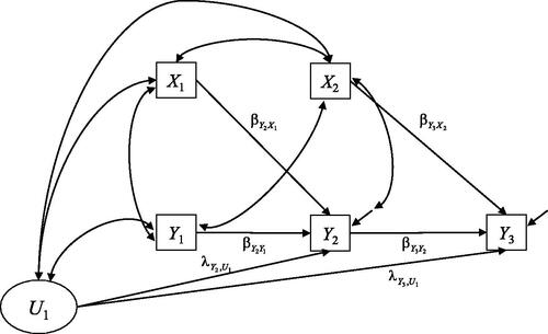
It should be emphasized that the FED does not provide estimates for the effects of $Y$ on $X.$ This has the advantage that no assumptions are made regarding the dependence structure of $X$ on $Y.$² However, if researchers are interested in reciprocal effects, they need to specify a separate model for $X$ that is analogous to Equation (25)(24) $$\left(\genfrac{}{}{0pt}{}{X_t}{Y_t}\right)=\left(\begin{array}{cc}{\mathrm{\beta }}_{X_t{X}_{t-1}}& {\mathrm{\beta }}_{X_t{Y}_{t-1}}\\ {\mathrm{\beta }}_{Y_t{X}_{t-1}}& {\mathrm{\beta }}_{Y_t{Y}_{t-1}}\end{array}\right)\left(\begin{array}{c}{X}_{t-1\mathrm{ }}\\ Y_{t-1\mathrm{ }}\end{array}\right)+\left(\begin{array}{cc}{\lambda }_{X_t,U_1}-{\mathrm{\beta }}_{X_t{X}_{t-1}}{\lambda }_{X_{t-1},U_1}& 0\\ 0& {\lambda }_{Y_t,U_2}-{\mathrm{\beta }}_{Y_t{Y}_{t-1}}{\lambda }_{Y_{t-1},U_2}\end{array}\right)\left(\genfrac{}{}{0pt}{}{U_1}{U_2}\right)+\left(\genfrac{}{}{0pt}{}{e_{X_t}}{e_{Y_t}}\right)$$(24) .

3.4. Relationship between the Residual-Level and Observation-Level Approaches

In this section, we further investigate the relationship between the observation-level and residual-level approaches (see also Andersen, 2021; Bollen & Curran, 2004; Hamaker, 2005; Hsiao, 2014; Usami, 2021; Usami, Murayama, et al., 2019). More specifically, we clarify the conditions under which the two approaches are equivalent. We consider a general residual-level model with occasion-specific, freely estimated loading matrices: (27) $${\mathbf{Z}}_1={\mathbf{\Lambda }}_1\mathbf{U}+{\mathbf{e}}_1$$(27) (28) $${\mathbf{Z}}_t={{\mathbf{B}}_{t,t-1}\mathbf{Z}}_{t-1}^W+{\mathbf{\Lambda }}_t\mathbf{U}+{\mathbf{e}}_t \mathrm{for}\mathrm{ }t\ge 2$$(28)

Note that we use ${\mathbf{Z}}_1^W={\mathbf{e}}_1,$ and that the dimension of $\mathbf{U}$ can be different from the dimension of ${\mathbf{Z}}_t.$ The general observation-level model is given by (29) $$\mathrm{Cov}\left({\mathbf{Z}}_1,\tilde{\mathbf{U}}\right)={\tilde{\mathbf{\Psi }}}_{{\mathbf{Z}}_1\tilde{\mathbf{U}}}$$(29) (30) $${\mathbf{Z}}_t={\tilde{\mathbf{B}}}_{t,t-1}{\mathbf{Z}}_{t-1}+{\tilde{\mathbf{\Lambda }}}_t\tilde{\mathbf{U}}+{\tilde{\mathbf{e}}}_t \text{ for }t\ge 2$$(30) where ${\tilde{\mathbf{B}}}_{t,t-1},$ ${\tilde{\mathbf{\Lambda }}}_t,$ ${\tilde{\mathbf{\Lambda }}}_1,$ $\tilde{\mathbf{U}},$ and ${\tilde{\mathbf{e}}}_t$ denote the parameters in the observation-level model. An important special case is the observation-level model in which the covariance of ${\mathbf{Z}}_1$ and $\tilde{\mathbf{U}}$ is represented as a loading matrix ${\tilde{\mathbf{\Lambda }}}_1$ (see Zyphur et al., 2020) (31) $${\mathbf{Z}}_1={\tilde{\mathbf{\Lambda }}}_1\tilde{\mathbf{U}}+{\tilde{\mathbf{e}}}_1$$(31)

In order to show that in the general case the two models are equivalent, we show that the parameters in Equations (27)(26) $$Y_t={\mathit{\beta }}_{Y_t{Y}_{t-1}}{Y}_{t-1}+{\mathrm{\beta }}_{Y_t{X}_{t-1}}{X}_{t-1}+{\mathrm{\lambda }}_{Y_t,U_1}{U}_1+e_t \mathrm{for}\mathrm{ }t\ge 2,$$(26) and (28)(27) $${\mathbf{Z}}_1={\mathbf{\Lambda }}_1\mathbf{U}+{\mathbf{e}}_1$$(27) can be represented as parameters in Equations (30)(29) $$\mathrm{Cov}\left({\mathbf{Z}}_1,\tilde{\mathbf{U}}\right)={\tilde{\mathbf{\Psi }}}_{{\mathbf{Z}}_1\tilde{\mathbf{U}}}$$(29) and (31)(30) $${\mathbf{Z}}_t={\tilde{\mathbf{B}}}_{t,t-1}{\mathbf{Z}}_{t-1}+{\tilde{\mathbf{\Lambda }}}_t\tilde{\mathbf{U}}+{\tilde{\mathbf{e}}}_t \text{ for }t\ge 2$$(30) , and vice versa.

3.4.1. Equivalence of General Residual-Level and Observation-Level Models

First, we start with the residual-level model and write Equation (28)(27) $${\mathbf{Z}}_1={\mathbf{\Lambda }}_1\mathbf{U}+{\mathbf{e}}_1$$(27) as follows (32) $${\mathbf{Z}}_t={\mathbf{B}}_{t,t-1}{\mathbf{Z}}_{t-1}+{(\mathbf{\Lambda }}_t-{\mathbf{B}}_{t,t-1}{\mathbf{\Lambda }}_{t-1})\mathbf{U}+{\mathbf{e}}_t \mathrm{ f}\mathrm{or} t\ge 2.$$(32)

By setting ${\tilde{\mathbf{B}}}_{t,t-1}\equiv {\mathbf{B}}_{t,t-1},$ ${\tilde{\mathbf{\Lambda }}}_t\equiv {\mathbf{\Lambda }}_t-{\mathbf{B}}_{t,t-1}{\mathbf{\Lambda }}_{t-1},$ $\tilde{\mathbf{U}}\equiv \mathbf{U},$ and ${\tilde{\mathbf{e}}}_t\equiv {\mathbf{e}}_t,$ we obtain Equation (30)(29) $$\mathrm{Cov}\left({\mathbf{Z}}_1,\tilde{\mathbf{U}}\right)={\tilde{\mathbf{\Psi }}}_{{\mathbf{Z}}_1\tilde{\mathbf{U}}}$$(29) of the observation-level approach. At $t=1,$ we can obviously set ${\tilde{\mathbf{\Lambda }}}_1\equiv {\mathbf{\Lambda }}_1,$ and ${\tilde{\mathbf{e}}}_1\equiv {\mathbf{e}}_1$ (see Equation (31)(30) $${\mathbf{Z}}_t={\tilde{\mathbf{B}}}_{t,t-1}{\mathbf{Z}}_{t-1}+{\tilde{\mathbf{\Lambda }}}_t\tilde{\mathbf{U}}+{\tilde{\mathbf{e}}}_t \text{ for }t\ge 2$$(30) ). Thus, the model parameters of the general residual-level model can be represented as parameters of the observation-level model.

Next, we start with an observation-level model (see Equations (30)(29) $$\mathrm{Cov}\left({\mathbf{Z}}_1,\tilde{\mathbf{U}}\right)={\tilde{\mathbf{\Psi }}}_{{\mathbf{Z}}_1\tilde{\mathbf{U}}}$$(29) and (31)(30) $${\mathbf{Z}}_t={\tilde{\mathbf{B}}}_{t,t-1}{\mathbf{Z}}_{t-1}+{\tilde{\mathbf{\Lambda }}}_t\tilde{\mathbf{U}}+{\tilde{\mathbf{e}}}_t \text{ for }t\ge 2$$(30) ). We now define ${\mathbf{B}}_{t,t-1}\equiv {\tilde{\mathbf{B}}}_{t,t-1},$$\mathrm{ }{\mathbf{\Lambda }}_1\equiv {\tilde{\mathbf{\Lambda }}}_1,$ $\mathbf{U}\equiv \tilde{\mathbf{U}},$ and ${\mathbf{e}}_t\equiv {\tilde{\mathbf{e}}}_t.$ We also set (33) $${\mathbf{\Lambda }}_t\mathrm{ }\equiv \mathrm{ }{\tilde{\mathbf{\Lambda }}}_t+{\tilde{\mathbf{B}}}_{t,t-1}{\mathbf{\Lambda }}_{t-1} \mathrm{ }\mathrm{for} t\ge 2$$(33)

For $t=2,$ we have ${\mathbf{\Lambda }}_{t-1}={\tilde{\mathbf{\Lambda }}}_1.$ For $t>2,$ ${\mathbf{\Lambda }}_{t-1}$ is a function of model parameters defined in Equations (30)(29) $$\mathrm{Cov}\left({\mathbf{Z}}_1,\tilde{\mathbf{U}}\right)={\tilde{\mathbf{\Psi }}}_{{\mathbf{Z}}_1\tilde{\mathbf{U}}}$$(29) and (31)(30) $${\mathbf{Z}}_t={\tilde{\mathbf{B}}}_{t,t-1}{\mathbf{Z}}_{t-1}+{\tilde{\mathbf{\Lambda }}}_t\tilde{\mathbf{U}}+{\tilde{\mathbf{e}}}_t \text{ for }t\ge 2$$(30) , that is ${\tilde{\mathbf{\Lambda }}}_t$ and ${\tilde{\mathbf{B}}}_{t,t-1}.$ This shows that the paramaters of the general observation-level model can be re-expressed as parameters of a residual-level model, and the two approaches are equivalent. Note that this would also hold true for the special case that the regression coefficients are invariant across time, that is ${\mathbf{B}}_{t,t-1}={\tilde{\mathbf{B}}}_{t,t-1}\equiv \mathbf{B}$ in Equations (28)(27) $${\mathbf{Z}}_1={\mathbf{\Lambda }}_1\mathbf{U}+{\mathbf{e}}_1$$(27) and (30)(29) $$\mathrm{Cov}\left({\mathbf{Z}}_1,\tilde{\mathbf{U}}\right)={\tilde{\mathbf{\Psi }}}_{{\mathbf{Z}}_1\tilde{\mathbf{U}}}$$(29) .

3.4.2. Representation of a Simple Structure Residual-Level Model as an Observation-Level Model

Next, we consider a residual-level model with time-invariant coefficients $\mathbf{B},$ and a diagonal, time-invariant loading matrix. This is a special version of the RI-CLPM (RL1) and can be written as (34) $${\mathbf{Z}}_1=\mathbf{\Lambda }\mathbf{U} + {\mathbf{e}}_1$$(34) (35) $${\mathbf{Z}}_t={\mathbf{BZ}}_{t-1}+(\mathbf{I}-\mathbf{B})\mathbf{\Lambda }\mathbf{U}+{\mathbf{e}}_t \mathrm{ f}\mathrm{or }t\ge 2.$$(35)

We show that this model can be represented as an observation-level model with a simple structure loading matrix for $t\ge 2.$ To this end, we define a diagonal matrix $\tilde{\mathbf{\Lambda }}$ and latent variables $\tilde{\mathbf{U}}$ by (36) $$\tilde{\mathbf{\Lambda }}\tilde{\mathbf{U}}\equiv (\mathbf{I}-\mathbf{B})\mathbf{\Lambda }\mathbf{U}$$(36)

Note that the only purpose of the diagonal matrix $\tilde{\mathbf{\Lambda }}$ is to standardize the components in $\tilde{\mathbf{U}}.$ Moreover, we can define for $t=1$ (37) $${\tilde{\mathbf{\Lambda }}}_1\equiv {\tilde{\mathbf{\Lambda }}}^{-1}(\mathbf{I}-\mathbf{B}{)}^{-1}\mathbf{\Lambda }.$$(37)

As $\mathbf{B}$ is typically nondiagonal, the loading matrix ${\tilde{\mathbf{\Lambda }}}_1$ at $t=1$ in the observation-level model is nondiagonal. Thus, a RI-CLPM with time-invariant regression coefficients (RL1) can be re-expressed as an observation-level model with a nondiagonal loading matrix ${\tilde{\mathbf{\Lambda }}}_1$ (OL2 in Equation (15)(15) $$\left(\begin{array}{c}{X}_t\\ Y_t\end{array}\right)=\left(\begin{array}{cc}{\mathrm{\beta }}_{X_t{X}_{t-1}}& {\mathrm{\beta }}_{X_t{Y}_{t-1}}\\ {\mathrm{\beta }}_{Y_t{X}_{t-1}}& {\mathrm{\beta }}_{Y_t{Y}_{t-1}}\end{array}\right)\left(\begin{array}{c}{X}_{t-1}\\ Y_{t-1}\end{array}\right)+\left(\begin{array}{cc}{\mathrm{\lambda }}_{X_t,U_1}& 0\\ 0& {\mathrm{\lambda }}_{Y_t,U_2}\end{array}\right)\left(\begin{array}{c}{U}_1\\ U_2\end{array}\right)+\left(\begin{array}{c}{e}_{X_t}\\ e_{Y_t}\end{array}\right) \mathrm{f}\mathrm{or} t\ge 2,$$(15) ; see Andersen, 2021). However, a RI-CLPM cannot, in general, be written as an observation-level model with a diagonal ${\tilde{\mathbf{\Lambda }}}_1$ (OL3 in Equation (16)(16) $$\left(\genfrac{}{}{0pt}{}{X_1}{Y_1}\right)=\left(\begin{array}{cc}{\lambda }_{X_1,U_1}& 0\\ 0& {\lambda }_{Y_1,U_2}\end{array}\right)\left(\genfrac{}{}{0pt}{}{U_1}{U_2}\right)+\left(\genfrac{}{}{0pt}{}{e_{X_1}}{e_{Y_1}}\right),$$(16) ).

3.4.3. Representation of a Simple Structure Observation-Level Model as a Residual-Level Model

We now start with an observation-level model (38) $${\mathbf{Z}}_1={\tilde{\mathbf{\Lambda }}}_1\tilde{\mathbf{U}}+{\tilde{\mathbf{e}}}_1$$(38) (39) $${\mathbf{Z}}_t=\tilde{\mathbf{B}}{\mathbf{Z}}_{t-1}+\tilde{\mathbf{\Lambda }}\tilde{\mathbf{U}}+{\tilde{\mathbf{e}}}_t \text{ for }t\ge 2,$$(39) where the matrix $\tilde{\mathbf{\Lambda }}$ is assumed to be diagonal (i.e., simple structure model). As pointed out before, the matrix ${\tilde{\mathbf{\Lambda }}}_1$ can be diagonal (OL3 in Equation (16)(16) $$\left(\genfrac{}{}{0pt}{}{X_1}{Y_1}\right)=\left(\begin{array}{cc}{\lambda }_{X_1,U_1}& 0\\ 0& {\lambda }_{Y_1,U_2}\end{array}\right)\left(\genfrac{}{}{0pt}{}{U_1}{U_2}\right)+\left(\genfrac{}{}{0pt}{}{e_{X_1}}{e_{Y_1}}\right),$$(16) ) or nondiagonal (OL2 in Equation (15)(15) $$\left(\begin{array}{c}{X}_t\\ Y_t\end{array}\right)=\left(\begin{array}{cc}{\mathrm{\beta }}_{X_t{X}_{t-1}}& {\mathrm{\beta }}_{X_t{Y}_{t-1}}\\ {\mathrm{\beta }}_{Y_t{X}_{t-1}}& {\mathrm{\beta }}_{Y_t{Y}_{t-1}}\end{array}\right)\left(\begin{array}{c}{X}_{t-1}\\ Y_{t-1}\end{array}\right)+\left(\begin{array}{cc}{\mathrm{\lambda }}_{X_t,U_1}& 0\\ 0& {\mathrm{\lambda }}_{Y_t,U_2}\end{array}\right)\left(\begin{array}{c}{U}_1\\ U_2\end{array}\right)+\left(\begin{array}{c}{e}_{X_t}\\ e_{Y_t}\end{array}\right) \mathrm{f}\mathrm{or} t\ge 2,$$(15) ). In order to represent Equations (38)(37) $${\tilde{\mathbf{\Lambda }}}_1\equiv {\tilde{\mathbf{\Lambda }}}^{-1}(\mathbf{I}-\mathbf{B}{)}^{-1}\mathbf{\Lambda }.$$(37) and (39)(38) $${\mathbf{Z}}_1={\tilde{\mathbf{\Lambda }}}_1\tilde{\mathbf{U}}+{\tilde{\mathbf{e}}}_1$$(38) as a residual-level model, we get defining equations (40) $${\mathbf{\Lambda }}_1\mathbf{U}={\tilde{\mathbf{\Lambda }}}_1\tilde{\mathbf{U}}$$(40) (41) $$\left({\mathbf{\Lambda }}_t-{\mathbf{B}}_{t,t-1}{\mathbf{\Lambda }}_{t-1}\right)\mathbf{U}=\tilde{\mathbf{\Lambda }}\tilde{\mathbf{U}} \text{ for }t\ge 2$$(41)

We now set ${\mathbf{B}}_{t,t-1}\equiv \tilde{\mathbf{B}},$ and obtain by iterating (42) $${\mathbf{\Lambda }}_t\mathbf{U}=\tilde{\mathbf{\Lambda }}\tilde{\mathbf{U}}+\tilde{\mathbf{B}}{\mathbf{\Lambda }}_{t-1}\mathbf{U}=\left(\mathbf{I}+\tilde{\mathbf{B}}+{\tilde{\mathbf{B}}}^2+\dots +{\tilde{\mathbf{B}}}^{t-2}\right)\tilde{\mathbf{\Lambda }}\tilde{\mathbf{U}}+{\tilde{\mathbf{B}}}^{t-1}{\mathbf{\Lambda }}_1\mathbf{U}$$(42)

We use the matrix Taylor series ${\left(\mathbf{I}-\tilde{\mathbf{B}}\right)}^{-1}\simeq \mathbf{I}+\tilde{\mathbf{B}}+{\tilde{\mathbf{B}}}^2+\dots +{\tilde{\mathbf{B}}}^k$ if $k$ is large enough. This finding is based on the assumption that ${\tilde{\mathbf{B}}}^k\to 0$ for $k$ large enough which holds for stationary processes. If we assume that ${\tilde{\mathbf{B}}}^k\approx 0$ for all $k\ge 2,$ we can use the approximation ${\mathbf{\Lambda }}_t\mathbf{U}\approx {\left(\mathbf{I}-\tilde{\mathbf{B}}\right)}^{-1}\tilde{\mathbf{\Lambda }}\tilde{\mathbf{U}}$ for $t\ge 3.$ Thus, we can assume a simple structure ${\mathbf{\Lambda }}_t=\mathbf{\Lambda }$ for $t\ge 3$ with (43) $$\mathbf{\Lambda }\mathbf{U}={\left(\mathbf{I}-\tilde{\mathbf{B}}\right)}^{-1}\tilde{\mathbf{\Lambda }}\tilde{\mathbf{U}}$$(43)

We now set $\mathbf{\Lambda }\equiv {\left(\mathbf{I}-\tilde{\mathbf{B}}\right)}^{-1}\tilde{\mathbf{\Lambda }}$ for $t\ge 3.$ For the first two time points, we get (44) $${\mathbf{\Lambda }}_1\mathbf{U}={\tilde{\mathbf{\Lambda }}}_1\tilde{\mathbf{U}}=\left({\tilde{\mathbf{\Lambda }}}_1{\tilde{\mathbf{\Lambda }}}^{-1}(\mathbf{I}-\tilde{\mathbf{B}})\mathbf{\Lambda }\right)\mathbf{U}$$(44) (45) $${\mathbf{\Lambda }}_2\mathbf{U}=\tilde{\mathbf{\Lambda }}\tilde{\mathbf{U}}+{\tilde{\mathbf{B}}\mathbf{\Lambda }}_1\mathbf{U}=\left(\left(\mathbf{I}-\tilde{\mathbf{B}}\right)\mathbf{\Lambda }+{\tilde{\mathbf{B}}\mathbf{\Lambda }}_1\right)\mathbf{U}$$(45)

We define ${\mathbf{\Lambda }}_1\equiv ({\tilde{\mathbf{\Lambda }}}_1{\tilde{\mathbf{\Lambda }}}^{-1}(\mathbf{I}-\tilde{\mathbf{B}})\mathbf{\Lambda })$ and ${\mathbf{\Lambda }}_2\equiv \left(\left(\mathbf{I}-\tilde{\mathbf{B}}\right)\mathbf{\Lambda }+{\tilde{\mathbf{B}}\mathbf{\Lambda }}_1\right).$ This shows that the observation-level model in Equations (38)(37) $${\tilde{\mathbf{\Lambda }}}_1\equiv {\tilde{\mathbf{\Lambda }}}^{-1}(\mathbf{I}-\mathbf{B}{)}^{-1}\mathbf{\Lambda }.$$(37) and (39)(38) $${\mathbf{Z}}_1={\tilde{\mathbf{\Lambda }}}_1\tilde{\mathbf{U}}+{\tilde{\mathbf{e}}}_1$$(38) can be approximately represented as a residual-level model with a simple structure loading matrix. However, the loading matrices at the first two time points (${\mathbf{\Lambda }}_1$ and ${\mathbf{\Lambda }}_2$) in this approximation are, in general, not diagonal. Thus, an observation-level model with a simple structure loading matrix cannot be re-expressed as a simple structure residual-level model.

3.4.4. Representation of a Residual-Level Model as a Fixed Effects Dynamic Panel Model

We show that a residual-level model can be represented as a fixed effects dynamic panel model (FED; Allison et al., 2017). We start with the bivariate residual-level model in Equation (24)(23) $$\left(\begin{array}{c}{X}_t^W\\ Y_t^W\end{array}\right)=\left(\begin{array}{cc}{\mathrm{\beta }}_{X_t{X}_{t-1}}& {\mathrm{\beta }}_{X_t{Y}_{t-1}}\\ {\mathrm{\beta }}_{Y_t{X}_{t-1}}& {\mathrm{\beta }}_{Y_t{Y}_{t-1}}\end{array}\right)\left(\begin{array}{c}{X}_{t-1}^W\\ Y_{t-1}^W\end{array}\right)+\left(\genfrac{}{}{0pt}{}{e_{X_t}}{e_{Y_t}}\right)\text{ for }t\ge 2$$(23) , and assume time-invariant regression coefficients (${\mathrm{\beta }}_{XX},$ ${\mathrm{\beta }}_{XY},$ ${\mathrm{\beta }}_{YY},$ and ${\mathrm{\beta }}_{YX}$), and time-invariant loadings (${\mathrm{\lambda }}_{X,U_1}$ and ${\mathrm{\lambda }}_{Y,U_2}$).

The corresponding FED is given by (for $t\ge 2$) (46) $$Y_t={\tilde{\mathrm{\lambda }}}_{Y,{\tilde{U}}_1}{\tilde{U}}_1+{\tilde{\mathrm{\beta }}}_{YY}{Y}_{t-1}+{\tilde{\mathrm{\beta }}}_{YX}{X}_{t-1}+{\tilde{e}}_{Y_t}$$(46)

We now define ${\tilde{\mathrm{\lambda }}}_{Y,{\tilde{U}}_1}{\tilde{U}}_1\equiv \left(1-{\mathrm{\beta }}_{YY}\right){\mathrm{\lambda }}_{Y,U_2}{U}_2-{\mathrm{\beta }}_{YX}{\mathrm{\lambda }}_{X,U_1}{U}_1,$ where ${\tilde{U}}_1$ is a standardized variable. Furthermore, we set ${\tilde{\mathrm{\beta }}}_{YY}\equiv {\mathrm{\beta }}_{YY},$ ${\tilde{\mathrm{\beta }}}_{YX}\equiv {\mathrm{\beta }}_{YX}$, and ${\tilde{e}}_{Y_t}\equiv e_{Y_t}$ for $t\ge 2.$ Thus, the RI-CLPM can be represented as a FED. However, as the FED does not specify restrictions regarding the dependence of $X$ on $Y,$ the FED cannot, in general, be represented as an observation-level model (Allison et al., 2017), which implies that it can also not, in general, be represented as a residual-level model.

3.4.5. Summary

Overall, the main results of this section can be summarized as follows. First, the general observation-level and residual-level approaches with freely estimated loadings are equivalent if the same number of latent variables is utilized (i.e., dimension of $\mathbf{U}$ is the same). Second, residual-level models with a simple structure time-invariant loading matrix and time-invariant regression coefficients can be represented as a simple structure observation-level model with time-invariant regression coefficients. However, this is only the case if the loading matrix at $t=1$ in the observation-level model is nondiagonal (see OL2), and not if it is diagonal (see OL3). Third, the simple structure observation-level model with time-invariant regression coefficients cannot be re-expressed as a simple structure residual-level model (see Equations (44)(43) $$\mathbf{\Lambda }\mathbf{U}={\left(\mathbf{I}-\tilde{\mathbf{B}}\right)}^{-1}\tilde{\mathbf{\Lambda }}\tilde{\mathbf{U}}$$(43) and (45)(44) $${\mathbf{\Lambda }}_1\mathbf{U}={\tilde{\mathbf{\Lambda }}}_1\tilde{\mathbf{U}}=\left({\tilde{\mathbf{\Lambda }}}_1{\tilde{\mathbf{\Lambda }}}^{-1}(\mathbf{I}-\tilde{\mathbf{B}})\mathbf{\Lambda }\right)\mathbf{U}$$(44) ), indicating that in the case of simple structure loading matrices, the observation-level approach is the more general approach (see Andersen, 2021). Fourth, both observation-level and residual-level models can be re-expressed as a fixed effects dynamic panel. However, in general, this is not possible the other way round (see Allison et al., 2017).

4. Estimation of Cross-Lagged Effects under Different Data-Generating Models

We now use simulated data to illustrate the conditions under which the different modeling approaches produce unbiased estimates of the cross-lagged effect. We distinguish four different scenarios for a cross-lagged panel design with three measurement waves and two variables (i.e., $X$ and $Y;$ see Figure 7). In Scenario A, we assumed that the true data-generating model was a CL2. In Scenario B, we assumed that the true model was an observation-level model with one latent variable (OL1). In Scenario C, the data were generated by residual-level models (RL1, RL2, and RL3). Finally, in Scenario D, we assumed that the true model was a fixed effects dynamic panel model (FED). For each scenario, we present the results for different data conditions generated under different parameters of the data-generating models. As we were only interested in the (large-sample) bias of the parameter estimates, we simulated only one large data set (N = 10000) for each data condition. In all scenarios, the variables (i.e., $X_1,$ $X_2,$ $X_3,$ $Y_1,$ $Y_2,$ $Y_3$) were standardized with zero means and variances of one. Our discussion focuses on the estimation of the (lag-1) cross-lagged effect of $X_2$ on $Y_3$ (i.e., ${\mathrm{\beta }}_{Y_3{X}_2}$). The R and lavaan (Rosseel, 2012) code for the data-generating models and the different analysis models is provided at https://bit.ly/3IN1FCi.

Figure 7. Four different simulation scenarios for a cross-lagged panel design with three measurement waves. Scenario A: true model is a cross-lagged panel model with lag-2 effects (CL2). Scenario B: true model is an observation-level model with a single latent variable (OL1). Scenario C: true model is a residual-level model. Scenario D: true model is a fixed effects dynamic panel model (FED).

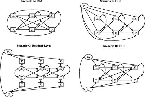
4.1. Scenario A: CL2 as the Data-Generating Model

In Scenario A, we assumed that the data were generated by a CL2 (see Equation (9)(9) $${\mathbf{Z}}_t={{\mathbf{B}}_{t,t-1}\mathbf{Z}}_{t-1}+{{\mathbf{B}}_{t,t-2}\mathbf{Z}}_{t-2}+{\mathbf{\Gamma }}_t\mathbf{C}+{\mathbf{e}}_t \text{ for }t\ge 2,$$(9) ). More specifically, we assumed a stationary process that fulfills a cross-lagged panel model with lag-2 effects (i.e., the lag-1 covariances were assumed to be constant for each data condition). We manipulated the lag-2 covariances by specifying different values for the lag-2 cross-lagged effects (i.e., ${\mathrm{\beta }}_{Y_3{X}_1}$), and the lag-2 autoregressive effects (i.e., ${\mathrm{\beta }}_{Y_3{Y}_1}$). This resulted in six different data conditions in which the synchronous and lag-1 correlations were constant, but the lag-2 correlations differed. We analyzed the six data sets with the cross-lagged panel model (CL1 and CL2), the four observation-level models (OL1, OL2, OL3, and OL4), the three residual-level models (RL1, RL2, and RL3), and the fixed effects dynamic panel model FED.

As expected, the CL2 that includes lag-2 effects provided unbiased estimates of the cross-lagged effect under all data conditions in this scenario (see Table 2). The CL1 produced positively biased estimates and overestimated the size of the true cross-lagged effect. For example, in condition A2 with small lag-2 cross-lagged effects (i.e., ${\mathrm{\beta }}_{Y_3{X}_1}$=.01), and a substantial lag-2 autoregressive effect (i.e., ${\mathrm{\beta }}_{Y_3{Y}_1}$=.32), the true cross-lagged effect is substantially overestimated in the CL1 (.20 vs. .10). This illustrates that the estimates of the CL1 can be strongly distorted by the presence of delayed effects that are not adequately captured by the lag-1 effects (VanderWeele et al., 2020; see also Marsh et al., 2018). Note that the estimated cross-lagged effects in the CL1 did not change across the data conditions because the lag-1 correlations were fixed, and only the lag-2 correlations were manipulated.

Table 2. Results for Scenario A: True model is the cross-lagged panel model with lag-2 effects (CL2). Estimates of the cross-lagged effect for the different approaches.

Dataset	${\mathrm{\beta }}_{Y_3{X}_1}$	${\mathrm{\beta }}_{Y_3{Y}_1}$	${\mathrm{\beta }}_{Y_3{X}_2}$	CL1	CL2	OL1	OL2	OL3	OL4	RL1	RL2	RL3	FED
A1	0.08	0.27	0.10	0.20	0.10	0.23	0.02	0.01	0.00	0.02	0.02	0.02	0.02
A2	0.01	0.32	0.10	0.20	0.10	0.20	0.05	−0.02	0.14	−0.02	0.22	−0.04	0.18
A3	0.04	0.29	0.12	0.20	0.12	0.23	0.08	0.04	0.00	0.08	0.08	0.08	0.08
A4	−0.01	0.33	0.12	0.20	0.12	0.19	0.11	−0.01	0.15	0.04	0.26	0.03	0.23
A5	0.03	0.27	0.14	0.20	0.14	0.14	0.14	0.08	0.15	0.15	0.25	0.13	0.05
A6	0.00	0.30	0.14	0.20	0.14	0.10	0.14	0.06	0.00	0.14	0.14	0.14	0.14

Note. CL1 = cross-lagged panel model with lag-1 effects; CL2 = cross-lagged panel model with lag-2 effects; OL1 = observation-level model with a single latent factor; OL2 = observation-level model with two latent variables and freely estimated correlations at time 1; OL3 = observation-level model with two latent variables and diagonal loading matrix at time 1; OL4 = OL3 with non-invariant loadings across time; RL1 = residual-level model with diagonal and time-invariant loading matrices and time-invariant regression coefficients; RL2 = RL1 with non-invariant loading matrices; RL3 = RL1 with freely estimated regression coefficients; FED = fixed effects dynamic panel model. ${\mathrm{\beta }}_{Y_3{X}_1}$ = true lag-2 cross-lagged effect of $X_1$ on $Y_3;$ ${\mathrm{\beta }}_{Y_3{Y}_1}$= true lag-2 autoregressive effect of $Y_1$ on $Y_3;$ ${\mathrm{\beta }}_{Y_3{X}_2}$ = true lag-1 cross-lagged effect of $X_2$ on $Y_3.$ Absolute biases for the estimates of the lag-1 cross-lagged effect larger than .02 are printed in bold.

Most importantly, the models that include additional latent variables to adjust for unmeasured confounding produced biased estimates that were sometimes too large and sometimes too small. For example, the estimates of the residual-level models strongly depended on the size of the lag-2 effects, and the RL3 tended to underestimate the magnitude of the true cross-lagged effect. In condition A2 (i.e., ${\mathrm{\beta }}_{Y_3{X}_1}$=.01, and ${\mathrm{\beta }}_{Y_3{Y}_1}$=.32), the estimate provided by the RL3 even had a different sign than the true cross-lagged effect (–.04 vs. .10). The bias of the residual-level models (RL1, RL2, and RL3) completely vanished when no lag-2 cross-lagged effect was present in the condition A6 (i.e., ${\mathrm{\beta }}_{Y_3{X}_1}$=0).

Overall, scenario A confirms findings from the methodological literature that the CL1 can positively bias estimates of cross-lagged effects because it provides insufficient control for confounding due to the lag-2 effects. It also shows that the additional latent variables in the observation-level and residual-level models capture these lag-2 effects. However, in general, they do not appropriately control for the confounding due to previous measures of the exposure and the outcome, resulting in biased estimates of cross-lagged effects.

4.2. Scenario B: OL1 as the Data-Generating Model

In Scenario B, we assumed that an observation-level model with a single latent variable is the data-generating model (OL1; see Equation (14)(14) $$\underset{{\mathbf{Z}}_t}{\underbrace{\left(\genfrac{}{}{0pt}{}{X_t}{Y_t}\right)}}=\underset{{\mathbf{B}}_{t,t-1}}{\underbrace{\left(\genfrac{}{}{0pt}{}{{\mathrm{\beta }}_{X_t{X}_{t-1}}}{{\mathrm{\beta }}_{Y_t{X}_{t-1}}}\genfrac{}{}{0pt}{}{{\mathrm{\beta }}_{X_t{Y}_{t-1}}}{{\mathrm{\beta }}_{Y_t{Y}_{t-1}}}\right)}}\underset{{\mathbf{Z}}_{t-1} }{\underbrace{\left(\genfrac{}{}{0pt}{}{X_{t-1}}{Y_{t-1}}\right)}}+\underset{{\mathbf{\Lambda }}_t}{\underbrace{\left(\genfrac{}{}{0pt}{}{{\mathrm{\lambda }}_{X_t,U_1}}{{\mathrm{\lambda }}_{Y_t,U_1}}\right)}}\underset{\mathbf{U}}{\underbrace{U_1}}+\underset{{\mathbf{e}}_t}{\underbrace{\left(\genfrac{}{}{0pt}{}{e_{X_t}}{e_{Y_t}}\right)}} \mathrm{f}\mathrm{or} t\ge 2,$$(14) ). We fixed the true value of the cross-lagged effect (${\mathrm{\beta }}_{Y_3{X}_2}$=.20) and manipulated the effect of the latent variable $U_1$ on the observed variables by assuming that the correlation between $U_1$ and $Y$ decreased by a factor of .50 (${\mathrm{\rho }}_{Y_1{U}_1}$=.50, ${\mathrm{\rho }}_{Y_2{U}_1}$=.25, and ${\mathrm{\rho }}_{Y_3{U}_1}$=.13), was constant across time (${\mathrm{\rho }}_{Y_1{U}_1}$=${\mathrm{\rho }}_{Y_2{U}_1}$=${\mathrm{\rho }}_{Y_3{U}_1}$=.50), or increased by a factor of 2 (${\mathrm{\rho }}_{Y_1{U}_1}$=.05, ${\mathrm{\rho }}_{Y_2{U}_1}$=.10, and ${\mathrm{\rho }}_{Y_3{U}_1}$=.20) or 3 (${\mathrm{\rho }}_{Y_1{U}_1}$=.05, ${\mathrm{\rho }}_{Y_2{U}_1}$=.15, and ${\mathrm{\rho }}_{Y_3{U}_1}$=.45). In addition, we assumed that the correlation between $U_1$ and $X$ decreased by a factor of .5 (${\mathrm{\rho }}_{X_1{U}_1}$=.30, ${\mathrm{\rho }}_{X_2{U}_1}$=.15, and ${\mathrm{\rho }}_{X_3{U}_1}$=.08) or was constant across time (${\mathrm{\rho }}_{X_1{U}_1}$= ${\mathrm{\rho }}_{X_2{U}_1}$= ${\mathrm{\rho }}_{X_3{U}_1}$=.30). Overall, this resulted in six data conditions.

Table 3 shows the results for the six data conditions. As expected, the observation-level model with a single latent variable (OL1) produced unbiased estimates of the cross-lagged effect. By contrast, the models that assume no unmeasured confounding (CL1 and CL2) and the other latent variable-type models provided positively or negatively biased estimates of the cross-lagged effect, depending on the effect of the latent variable $U_1$ in the true data-generating model. For example, in condition B6 in which $U_1$ had an increasing effect across time on $Y,$ the estimates of CL1 and CL2 were positively biased (CL1: .29, CL2: .27), while many of the estimates provided by the latent variable-type models were negatively biased (OL2: .16, OL3: .17, RL2: .05, FED: −.01). The estimate of the RL1 was unbiased in this condition but was too small in condition B4, in which $U_1$ had a decreasing effect across time on $Y.$ Interestingly, the estimates produced by the observation-level model OL4 were almost unbiased. This indicates that, at least in the investigated conditions, the freely estimated loadings in OL4 can capture the time-varying (linear) effect of a single unmeasured variable.

Table 3. Results for Scenario B: True model is the observation-level model with single latent variable (OL1). Estimates of the cross-lagged effect for the different approaches.

Dataset	${\mathrm{\rho }}_{Y_1{U}_1}$	${\mathrm{\rho }}_{Y_2{U}_1}$	${\mathrm{\rho }}_{Y_3{U}_1}$	${\mathrm{\rho }}_{X_1{U}_1}$	${\mathrm{\rho }}_{X_2{U}_1}$	${\mathrm{\rho }}_{X_3{U}_1}$	${\mathrm{\beta }}_{Y_3{X}_2}$	CL1	CL2	OL1	OL2	OL3	OL4	RL1	RL2	RL3	FED
B1	0.50	0.50	0.50	0.30	0.30	0.30	0.20	0.21	0.20	0.20	0.20	0.20	0.20	0.20	0.20	0.20	0.20
B2	0.50	0.50	0.50	0.30	0.15	0.08	0.20	0.17	0.16	0.21	0.19	0.18	0.18	0.19	0.21	0.17	0.18
B3	0.50	0.25	0.13	0.30	0.15	0.08	0.20	0.20	0.20	0.20	0.17	0.18	0.20	0.20	0.15	0.20	0.19
B4	0.50	0.25	0.13	0.30	0.30	0.30	0.20	0.19	0.19	0.20	0.17	0.19	0.19	0.14	0.20	0.14	0.20
B5	0.05	0.10	0.20	0.30	0.30	0.30	0.20	0.23	0.22	0.20	0.18	0.19	0.20	0.21	0.17	0.22	0.14
B6	0.05	0.15	0.45	0.30	0.30	0.30	0.20	0.29	0.27	0.20	0.16	0.17	0.20	0.21	0.05	0.25	–0.01

Note. CL1 = cross-lagged panel model with lag-1 effects; CL2 = cross-lagged panel model with lag-2 effects; OL1 = observation-level model with a single latent factor; OL2 = observation-level model with two latent variables and freely estimated correlations at time 1; OL3 = observation-level model with two latent variables and diagonal loading matrix at time 1; OL4 = OL3 with non-invariant loadings across time; RL1 = residual-level model with diagonal and time-invariant loading matrices and time-invariant regression coefficients; RL2 = RL1 with non-invariant loading matrices; RL3 = RL1 with freely estimated regression coefficients; FED = fixed effects dynamic panel model. ${\mathrm{\rho }}_{Y_1{U}_1}$= true correlation between $Y_1$ and $U_1;$ ${\mathrm{\rho }}_{Y_2{U}_1}$ = true correlation between $Y_2$ and $U_1;$ ${\mathrm{\rho }}_{Y_3{U}_1}$ = true correlation between $Y_3$ and $U_1;$ ${\mathrm{\rho }}_{X_1{U}_1}$ = true correlation between $X_1$ and $U_1;$ ${\mathrm{\rho }}_{X_2{U}_1}$ = true correlation between $X_2$ and $U_1;$ ${\mathrm{\rho }}_{X_3{U}_1}$ = true correlation between $X_3$ and $U_1;$ ${\mathrm{\beta }}_{Y_3{X}_2}$ = true cross-lagged effect of $X_2$ on $Y_3$ in the data-generating model OL1. Absolute biases for the estimates of the cross-lagged effect larger than .02 are printed in bold.

Table 4. Results for Scenario C: True Model is the residual-level (RL) Model. Estimates for the cross-lagged effect for the different approaches.

Dataset	${\mathrm{\varphi }}_{U_1}$	${\mathrm{\beta }}_{Y_2{X}_1}$	${\mathrm{\lambda }}_{Y_2,U_2}$	${\mathrm{\beta }}_{Y_3{X}_2}$	CL1	CL2	OL1	OL2	OL3	OL4	RL1	RL2	RL3	FED
C1	0.30	0.20	1.00	0.20	0.13	0.17	0.24	0.20	0.15	0.09	0.20	0.20	0.20	0.20
C2	0.50	0.20	1.00	0.20	0.12	0.16	0.27	0.20	0.12	0.02	0.20	0.20	0.20	0.20
C3	0.70	0.20	1.00	0.20	0.11	0.15	0.29	0.20	0.07	−0.02	0.20	0.20	0.20	0.20
C4	0.30	0.05	1.00	0.20	0.13	0.15	0.02	0.00	0.10	0.02	0.11	0.04	0.19	−0.10
C5	0.50	0.05	1.00	0.20	0.12	0.15	0.15	0.01	0.07	0.04	0.12	0.03	0.19	−0.10
C6	0.70	0.05	1.00	0.20	0.11	0.13	0.23	0.05	0.03	0.05	0.12	0.18	0.19	−0.10
C7	0.30	0.20	0.80	0.20	0.13	0.16	0.16	0.19	0.18	0.16	0.20	0.20	0.20	0.17
C8	0.50	0.20	0.80	0.20	0.13	0.15	0.11	0.17	0.16	0.09	0.22	0.20	0.22	0.14
C9	0.70	0.20	0.80	0.20	0.12	0.14	0.07	0.14	0.13	0.03	0.25	0.20	0.25	0.10

Note. CL1 = cross-lagged panel model with lag-1 effects; CL2 = cross-lagged panel model with lag-2 effects; OL1 = observation-level model with a single latent factor; OL2 = observation-level model with two latent variables and freely estimated correlations at time 1; OL3 = observation-level model with two latent variables and diagonal loading matrix at time 1; OL4 = OL3 with non-invariant loadings across time; RL1 = residual-level model with diagonal and time-invariant loading matrices and time-invariant regression coefficients; RL2 = RL1 with non-invariant loading matrices; RL3 = RL1 with freely estimated regression coefficients; FED = fixed effects dynamic panel model. ${\mathrm{\varphi }}_{U_1}$= Variance of $U_1;$ ${\mathrm{\beta }}_{Y_2{X}_1}$ = true lag-1 cross-lagged effect of $X_1$ on $Y_2;$ ${\mathrm{\lambda }}_{Y_2,U_2}$= loading of $Y_2$ on $U_2$ (0.80 indicates that loadings are noninvariant across time); ${\mathrm{\beta }}_{Y_3{X}_2}$ = true lag-1 cross-lagged effect of $X_2$ on $Y_3$ in the residual-level model. Absolute biases for the estimates of the lag-1 cross-lagged effect larger than .02 are printed in bold.

4.3. Scenario C: Residual-Level Model as the Data-Generating Model

In Scenario C, we assumed that a residual-level model is a data-generating model with a true cross-lagged effect of ${\mathrm{\beta }}_{Y_3{X}_2}$=.20. The correlation of the latent variables was set to .6 (i.e., ${\mathrm{\rho }}_{U_1{U}_2}$=.60), We manipulated the variance of the between-person part of $X$ (i.e., ${\mathrm{\varphi }}_{U_1}$=.30, .50, and .70), the cross-lagged effect of $X_1$ on $Y_2$ (${\mathrm{\beta }}_{Y_2{X}_1}$=.20 vs. ${\mathrm{\beta }}_{Y_2{X}_1}$=.05), and the loadings of $Y$ on $U_2$ (${\lambda }_{Y_1,U_2}$=${\lambda }_{Y_2,U_2}$=${\lambda }_{Y_3,U_2}$=1.00 vs. ${\lambda }_{Y_1,U_2}$=1.00, ${\lambda }_{Y_2,U_2}$=.80, and ${\lambda }_{Y_3,U_2}$=.64). This resulted in nine different data conditions in which the regression coefficients and loadings were invariant across time (C1, C2, and C3), the regression coefficients were different, but the loadings were the same across time (C4, C5, and C6), and the regression coefficients were invariant, but the loadings differ across time (C7, C8, and C9).

As expected, the residual-level models could produce unbiased estimates of the cross-lagged effect in all nine conditions (Table 4). However, the estimates of RL1 and RL2 were biased when the true regression coefficients were not invariant across time (conditions C4, C5, C6), and only RL3 with freely estimated loadings provided unbiased estimates when the true loadings were allowed to vary across time in the data-generating model (conditions C7, C8, C9). As shown in the section “Relationship between the Residual-Level and Observation-Level Approaches”, the OL2 and FED are re-expressions of the residual-level models and produced identical estimates. However, this is no longer the case if the OL2 and FED are misspecified in conditions C4 to C9. Furthermore, the observation-level models with a simple structure loading matrix at time 1 (OL3 and OL4) produced negatively biased estimates of the cross-lagged effect across all conditions.

The estimates of the CL1 were consistently too small and underestimated the true magnitude of the cross-lagged effect, particularly when the variance of the between-person parts was large (i.e., ${\mathrm{\varphi }}_{U_1}$=.7). These findings replicated the results from Hamaker et al. (2015) and other simulation studies (Usami, Todo, et al., 2019) that the CL1 can produce distorted estimates of cross-lagged effects when the true data-generating model is an RL3. In addition, the CL2 that includes the lag-2 effects also produced estimates that underestimated the true magnitude of the cross-lagged effect. The bias for the CL2 was smaller but followed a similar pattern as the bias of the CL1.

4.4. Scenario D: FED as the Data-Generating Model

In Scenario D, we assumed that the fixed effects dynamic panel model FED is the true model. The data were generated from an observation-level model with two latent variables that were assumed to be correlated (${\mathrm{\rho }}_{U_1{U}_2}$=.60). We manipulated the variance of $U_1$ (i.e., ${\mathrm{\varphi }}_{U_1}$=.50 and .70), the loading of $X_3$ on $U_1$ (i.e.,${\lambda }_{X_3,U_1}$=0.15 and .50), and the lag-2 effect of $Y_1$ on $X_3$ (${\mathrm{\beta }}_{X_3{Y}_1}$=.0 and .07). This resulted in eight different conditions in which we varied the complexity in the $X$ part of the data by allowing for different loadings of $X$ on $U_1$ across time (conditions D3 and D4), additional lag-2 effects of $Y$ on $X$ (conditions D5 and D6), or both (conditions D7 and D8).

Table 5 shows that the FED produced unbiased estimates of the cross-lagged effect in all conditions. However, the estimates of the observation-level models (OL2, OL3, and OL4) were only unbiased if the loadings were invariant and no lag-2 effects were present in the data-generating model (conditions D1 and D2). This clearly illustrates that the FED can be interpreted as a more robust version of the observation-level models, and that the FED is to be prefered if researchers are only interested in estimating the cross-lagged effect but not in modeling the joint process of $X$ and $Y.$ The CL1 and CL2 overestimated the true magnitude of the cross-lagged effect and produced positively biased estimates across all conditions. Furthermore, the estimates of the residual-level models were strongly biased, even in the conditions with invariant loadings and no lag-2 effects (D1 and D2).

Table 5. Results for Scenario D: True model is the fixed effects dynamic panel model (FED). Estimates for the cross-lagged effect for the different approaches.

Dataset	${\mathrm{\varphi }}_{U_1}$	${\mathrm{\lambda }}_{X_3,U_1}$	${\mathrm{\beta }}_{X_3{Y}_1}$	${\mathrm{\beta }}_{Y_3{X}_2}$	CL1	CL2	OL1	OL2	OL3	OL4	RL1	RL2	RL3	FED
D1	0.5	0.5	0	0.20	0.21	0.23	0.20	0.20	0.20	0.20	0.27	0.27	0.27	0.20
D2	0.7	0.5	0	0.20	0.25	0.29	0.27	0.20	0.20	0.19	0.39	0.17	0.41	0.20
D3	0.5	0.15	0	0.20	0.21	0.23	0.19	0.22	0.23	0.20	0.26	0.30	0.26	0.20
D4	0.7	0.15	0	0.20	0.25	0.29	0.24	0.25	0.27	0.20	0.32	0.38	0.32	0.20
D5	0.5	0.5	0.07	0.20	0.21	0.23	0.22	0.09	0.14	0.15	0.19	0.08	0.22	0.20
D6	0.7	0.5	0.07	0.20	0.25	0.29	0.24	−0.03	0.08	0.12	−0.02	0.00	0.33	0.20
D7	0.5	0.15	0.07	0.20	0.21	0.23	−0.41	0.20	0.20	0.23	0.22	0.25	0.22	0.20
D8	0.7	0.15	0.07	0.20	0.25	0.29	0.43	0.23	0.26	0.25	0.28	0.34	0.28	0.20

Note. CL1 = cross-lagged panel model with lag-1 effects; CL2 = cross-lagged panel model with lag-2 effects; OL1 = observation-level model with a single latent factor; OL2 = observation-level model with two latent variables and freely estimated correlations at time 1; OL3 = observation-level model with two latent variables and diagonal loading matrix at time 1; OL4 = OL3 with non-invariant loadings across time; RL1 = residual-level model with diagonal and time-invariant loading matrices and time-invariant regression coefficients; RL2 = RL1 with non-invariant loading matrices; RL3 = RL1 with freely estimated regression coefficients; FED = fixed effects dynamic panel model. ${\mathrm{\varphi }}_{U_1}$= Variance of $U_1;$ ${\mathrm{\lambda }}_{X_3,U_1}$= loading of $X_3$ on $U_1$ (0.15 indicates that loadings are noninvariant across time); ${\mathrm{\beta }}_{X_3{Y}_1}$= true lag-2 cross-lagged effect of $Y_1$ on $X_3;$ ${\mathrm{\beta }}_{Y_3{X}_2}$ = true lag-1 cross-lagged effect of $X_2$ on $Y_3$ in the fixed effects dynamic panel model FED. Absolute biases for the estimates of the lag-1 cross-lagged effect larger than .02 are printed in bold.

4.5. Summary

The main findings of the simulations can be summarized as follows. First, when the CL2 was the true model (Scenario A), the estimates of the different latent variable-type models were biased in many conditions, indicating that the additional latent variables did not appropriately control for the lag-2 effects in the data-generating model. This shows that the potential to adjust for the effects of unmeasured variables comes with the price that the estimates of the latent variable methods are very sensitive to the parametric modeling assumptions needed for identifying the effects of the latent variables. Second, CL1 and CL2 produced biased estimates in the three scenarios in which unmeasured latent variables were included in the data-generating models (Scenarios B, C, and D). This was expected for CL1 and CL2 because these models rely on the assumption of no unmeasured confounding (i.e., all relevant covariates are measured). However, the results in these scenarios also show that the latent variable methods (OL1, OL2, OL3, OL4, RL1, RL2, RL3, and FED) strongly depended on the specific modeling assumptions made for estimating the effects of $\mathbf{U}.$ If these assumptions did not correspond with the data-generating model, they produced, in general, biased estimates of the cross-lagged effect. In practical applications with real data, the decision between the different approaches cannot be guided by model fit because different model specifications (with different estimates of the cross-lagged effect) will often provide an adequate description of the data (see Section “Limitations of Model Fit for Estimating Cross-Lagged Effects”). Third, the FED that is agnostic about the process of the exposure variable $X$ was less sensitive to specific modeling assumptions (see Allison et al., 2017) when estimating cross-lagged effects in the presence of unmeasured confounding. The estimates of the FED were biased in scenarios (B5, B6, and C4 to C9), in which specific parameter restrictions were needed for identifying the model (i.e., equal regression coefficients and loadings across time). With more measurement waves, these restrictions can be relaxed, and the FED would provide unbiased estimates in Scenarios B, C, and D. However, this would not resolve the central issue of scenario A because the FED still needs to make assumptions about the process of $Y$ for identifying the unit effects of $U_1.$

5. The Role of Time for Estimating the Causal Cross-Lagged Effect

In this section, we discuss the crucial role of selecting time points in defining the cross-lagged effect of interest (e.g., Gollob & Reichardt, 1987). We assume that the target of inference is the causal cross-lagged effect of $X_2$ on $Y_3,$ and we adjust for $X_1,$ $Y_1,$ and $Y_2$ in defining ${\mathrm{\tau }}_{{\mathcal{T}}_{X,Y},\mathrm{ACE}},$ that is ${\mathcal{T}}_X=\left\{1\right\}$ and ${\mathcal{T}}_Y=\left\{1,2\right\}.$ In the following, we assume that there are no unmeasured confounders. The bivariate process ${\mathbf{Z}}_t=(X_t,Y_t)$ (for $t\in \mathbb{R}$) is allowed to have an arbitrary dependency structure. We assume that ${\mathbf{Z}}_t$ follows a Gaussian process. Hence, the vector $\mathbf{Z}=({\mathbf{Z}}_{t_1},\dots ,{\mathbf{Z}}_{t_H})$ for H discrete time points $t_1,\dots ,t_H$ is multivariate normally distributed. The only requirement is that the values of ${\mathbf{Z}}_t$ only depend on the past; that is, they depend on ${\mathbf{Z}}_s$ with $s<t.$ It is important to emphasize that a continuous-time process ${\mathbf{Z}}_t$ should be considered as the underlying data-generating model. However, a longitudinal design of discrete time points is chosen to define model parameters (i.e., including the causal effect) of interest. 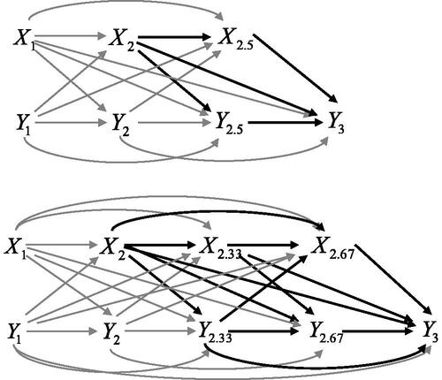Notably, a finite-dimensional parameter of a discrete-time process in a longitudinal design is a summary of the continuous-time process ${\mathbf{Z}}_t$ that can even depend on an infinite-dimensional parameter. In the following, we discuss the implications of choosing a particular longitudinal design by demonstrating that the model parameters in this design are functions of model parameters in a model with a refined grid of time points. By doing so, we clarify that the chosen time lags for defining the causal effect determine which effects (i.e., pathways) are controlled and which are part of the definition of the causal effect.

It is essential to understand that ${\mathrm{\tau }}_{{\mathcal{T}}_{X,Y},\mathrm{ACE}}$ includes all effects of $X_2$ on $Y_3$ that are transmitted via intermediated pathways between $X_2$ and $Y_3.$ This is illustrated in Figure 8 (upper panel), in which we consider the process at a refined grid of time points 1, 2, 2.5, and 3. As can be seen, the total effect of $X_2$ on $Y_3$ is transmitted via pathways ${X_2\to Y}_{2.5}\to Y_3$, ${X_2\to X}_{2.5}\to Y_3$ and $X_2\to Y_3$ (Keogh et al., 2018). More formally, the causal cross-lagged effect contains a direct effect ${\mathrm{\gamma }}_{Y_3{X}_2}$ and two indirect effects: (47) $${\mathrm{\tau }}_{{\mathcal{T}}_{X,Y},\mathrm{ACE}}={\mathrm{\gamma }}_{Y_3{X}_2}+{\mathrm{\gamma }}_{Y_3{X}_{2.5}}{\mathrm{\gamma }}_{X_{2.5}{X}_2}+{\mathrm{\gamma }}_{Y_3{Y}_{2.5}}{\mathrm{\gamma }}_{Y_{2.5}{X}_2}.$$(47)

Figure 8. Process of X_t and Y_t considered at time points 1, 2, 2.5, and 3 (upper panel), and time points 1, 2, 2.33, 2.67, and 3 (lower panel). Thick paths are included in the causal cross-lagged effect of X₂ on Y₃ (with adjustment for X₁, Y₁, and Y₂).

In most applications, the total effect ${\mathrm{\tau }}_{{\mathcal{T}}_{X,Y},\mathrm{ACE}}$ will differ from the direct effect ${\mathrm{\gamma }}_{Y_3{X}_2}$ as well as the coefficient ${\mathrm{\gamma }}_{Y_3{X}_{2.5}},$ which is based on a shorter time lag. This highlights the fact that the causal cross-lagged effect is independently defined from a particular process model, and that the causal effect of interest will not necessarily correspond to a regression coefficient in a well-fitting process model. To put it more clearly, it is not a question of model fit whether a researcher should report the total effect ${\mathrm{\tau }}_{{\mathcal{T}}_{X,Y},\mathrm{ACE}}$ from Equation (47)(46) $$Y_t={\tilde{\mathrm{\lambda }}}_{Y,{\tilde{U}}_1}{\tilde{U}}_1+{\tilde{\mathrm{\beta }}}_{YY}{Y}_{t-1}+{\tilde{\mathrm{\beta }}}_{YX}{X}_{t-1}+{\tilde{e}}_{Y_t}$$(46) (referring to $X_2\to Y_3$ with a time lag of 1) or ${\mathrm{\gamma }}_{Y_3{X}_{2.5}}$ (referring to $X_{2.5}\to Y_3$ with a time lag of 0.5).

The cross-lagged effect ${\mathrm{\tau }}_{{\mathcal{T}}_{X,Y},\mathrm{ACE}}$ can also be transmitted through pathways that include effects of $Y$ on $X.$ We also consider the process at time points 1, 2, 2.33, 2.67, and 3 (see lower panel in Figure 8). As can be seen, the indirect effect via ${X_2\to Y}_{2.33}\to {X_{2.67}\to Y}_3$ would be part of the total effect ${\mathrm{\tau }}_{{\mathcal{T}}_{X,Y},\mathrm{ACE}}.$ Thus, the cross-lagged effect at a single point in time targets the total effect that is transmitted through all (indirect and direct) paths between $X_2$ and $Y_3$ (Keogh et al., 2018).

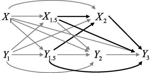
The longitudinal design also plays a crucial role when adjusting for previous exposure and outcome measures. We now consider the process at time points 1, 1.5, 2, and 3 (see Figure 9). As can be seen, with adjustment for $X_1,$ $Y_1,$ and $Y_2,$ the cross-lagged effect ${\mathrm{\tau }}_{{\mathcal{T}}_{X,Y},\mathrm{ACE}}$ includes effects of $X_{1.5}$ (i.e., $X_2\leftarrow {X_{1.5}\to Y}_3$) and $Y_{1.5}$ (i.e., $X_2\leftarrow {Y_{1.5}\to Y}_3$) if they exist. The causal effect can be calculated as (48) $${\mathrm{\tau }}_{{\mathcal{T}}_{X,Y},\mathrm{ACE}}={\mathrm{\gamma }}_{Y_3{X}_2}+{\mathrm{\gamma }}_{Y_3{X}_{1.5}}{\mathrm{\gamma }}_{X_2{X}_{1.5}}+{\mathrm{\gamma }}_{Y_3{Y}_{1.5}}{\mathrm{\gamma }}_{X_2{Y}_{1.5}}$$(48)

Figure 9. Process of X_t and Y_t considered at time points 1, 1.5, 2, and 3. Thick paths are included in the causal cross-lagged effect of X₂ on Y₃ (with adjustment for X₁, Y₁, and Y₂).

Given this reasoning, it might be tempting to adjust for additional covariates $X_{1.5}$ and $Y_{1.5};$ that is, one would utilize ${\mathcal{T}}_X=\left\{1,1.5\right\}$ and ${\mathcal{T}}_Y=\left\{1,1.5,2\right\}$ for defining an alternative causal effect. In this case, the prior levels of the exposure (i.e., $X_{1.5}$) would be treated as a confounder, and the causal effect would be ${\mathrm{\gamma }}_{Y_3{X}_2},$ which typically differs from ${\mathrm{\tau }}_{{\mathcal{T}}_{X,Y},\mathrm{ACE}}$ computed in Equation (48)(47) $${\mathrm{\tau }}_{{\mathcal{T}}_{X,Y},\mathrm{ACE}}={\mathrm{\gamma }}_{Y_3{X}_2}+{\mathrm{\gamma }}_{Y_3{X}_{2.5}}{\mathrm{\gamma }}_{X_{2.5}{X}_2}+{\mathrm{\gamma }}_{Y_3{Y}_{2.5}}{\mathrm{\gamma }}_{Y_{2.5}{X}_2}.$$(47) . As a consequence, the decision of a researcher to choosing ${\mathcal{T}}_X=\left\{1\right\}$ instead of ${\mathcal{T}}_X=\left\{1,1.5\right\}$ implies that in the former case, intermediate paths (i.e., the path $X_2\leftarrow {X_{1.5}\to Y}_3$) are also part of the causal effect of interest. Only controlling for $X_1$ does not rule out the possibility that intermediate exposures $X_u$ with 1<$u$<2 also contribute to the causal effect, where the contribution strongly depends on the correlation of $X_u$ with $X_2.$ This tradeoff in deciding whether to adjust for a previous exposure variable cannot be resolved by statistical modeling techniques (see VanderWeele et al., 2020, for a discussion of reasons to control for prior measures of $X$). For example, even in the case that a previous measure of the exposure received a statistically significant coefficient in a particular (process) model, it is still a conceptual question whether this covariate should serve as a control variable in the definition of the causal effect ${\mathrm{\tau }}_{{\mathcal{T}}_{X,Y},\mathrm{ACE}}.$

One interesting feature of Figures 8 and 9 is that the time grid can be arbitrarily refined. One may argue that this is a perfect showcase for continuous-time structural equation modeling (CTSEM; van Montfort et al., 2018), and that the challenge of selecting appropriate time points can be circumvented by using CTSEM. However, we are less convinced about the benefits of CTSEM because most of the applications discussed in the methodological literature only consider CTSEM relying on the Markov property (i.e., CTSEM without memory), which boils down to a specification of a lag-1 model with a tiny time lag. Thus, we believe that CTSEM with the Markov property cannot adequately model the dependence structure of time points and will typically be misspecified. Given these limitations, whether CTSEM offers significant advantages over discrete-time models in assessing causal cross-lagged effects can be questioned.

6. Limitations of Model Fit for Estimating Cross-Lagged Effects

In this section, we discuss whether the assessment of model fit could help to choose between the different modeling approaches for estimating cross-lagged effects. Our main argument is that the assessment of model fit is only of limited usefulness because the different modeling approaches provide almost equivalent representations of the observed covariance structure. As the residual-level and observation-level models are very similar (see section 3.4 “Relationship Between the Residual-Level and Observation-Level Approaches”), we restrict our discussion to the residual-level approach.

Under a multivariate normal distribution, only the fit of an observed covariance matrix $\mathbf{S}$ to a model-implied covariance matrix $\mathbf{\Sigma }$ is investigated. In the residual-level approach, the covariance structure of the observations at all time points, that is $\mathbf{\Sigma } = \mathrm{Var}(\mathbf{Z})$ for $\mathbf{Z}=({\mathbf{Z}}_1,\dots ,{\mathbf{Z}}_T)$ is decomposed as follows (49) $$\mathbf{\Sigma }={\mathbf{\Sigma }}_B+{\mathbf{\Sigma }}_W,$$(49) where ${\mathbf{\Sigma }}_B=\mathrm{Var}({\mathbf{Z}}^B)$ is the covariance matrix of the between-person part, that is ${\mathbf{Z}}^B = ({\mathbf{Z}}_1^B,\dots ,{\mathbf{Z}}_T^B)$ in Equation (18)(18) $${\mathbf{Z}}_t^B={{\mathbf{\Gamma }}_t\mathbf{C}+\mathbf{\Lambda }}_t\mathbf{U} \mathrm{for}\mathrm{ }t=1,\dots ,T$$(18) , and ${\mathbf{\Sigma }}_W=\mathrm{Var}({\mathbf{Z}}^W)$ of the within-person part, that is ${\mathbf{Z}}^W = ({\mathbf{Z}}_1^W,\dots ,{\mathbf{Z}}_T^W)$ in Equations (19)(19) $${\mathbf{Z}}_1^W={\mathbf{e}}_1 \text{ for }t=1$$(19) and (20)(20) $${ \mathbf{Z}}_t^W={{\mathbf{B}}_{t,t-1}\mathbf{Z}}_{t-1}^W+{\mathbf{e}}_t \text{ for }t\ge 2$$(20) . The causal cross-lagged effect is determined from the within-person part and, hence, is a parameter that affects the model-implied constrained covariance matrix ${\mathbf{\Sigma }}_W.$ For evaluating the assessment of global model fit, it is crucial that the model specification of the between-person part of the model is typically not independent of the specification of the within-person part. More specifically, a similar overall model fit for the total covariance $\mathbf{\Sigma }$ is obtained if the model for the between-person part is made more complex (e.g., by including time-varying loadings or random slopes), while the model for the within-person part is less complex (e.g., by specifying invariant lag-1 effects). If distinct freely estimated model parameters refer to ${\mathbf{\Sigma }}_B$ and ${\mathbf{\Sigma }}_W,$ then a total number of degrees of freedom $d{f}_0$ associated with the population covariance $\mathbf{\Sigma }$ can be used for modeling the between-person part (i.e., using $p_B^{}$ parameters) and the within-person part (i.e., using $p_W^{}$ parameters). The resulting degrees of freedom $df$ for the fitted residual-level model is given by (50) $$df=d{f}_0-p_B-p_W.$$(50)

Thus, if the number of parameters $p_B$ for the between-person part is increased, the number of within-person part parameters $p_W^{}$ needs to be reduced to obtain the same number of degrees of freedom $df.$³ This illustrates that the modeled complexity of one part of the model typically affects the required complexity of the other part of the model. However, the regression parameters for the within-person part will have different interpretations, depending on the specification of the model of the between-person and within-person parts, even though the overall model fit is the same for the different specifications (see Usami, Murayama, et al., 2019).

The limited usefulness of model fit was also evident in Scenario A of the simulation in which the CL2 was the true data-generating model. In this scenario, the residual-level model RL3 included stable traits with time-invariant loadings for the between-person part and assumed an AR(1) process for the within-person part. The CL2 did not model the between-person structure but assumed an AR(2) process. Both models showed a very similar fit, but the parameter estimates were very different. In such a constellation, the discussion of bias depends on how the true data-generating process is defined, and researchers cannot rely on model fit to choose between the CL2 or RL3. Consequently, the bias of a causal effect estimate from a particular model is entirely unrelated to its model fit.

It should be noted that the residual-level models contain some degrees of freedom and can be rejected based on model fit. However, in an application, researchers would modify their particular specification of the residual-level model to obtain a better-fitting model (e.g., freely estimated loadings). Successively using this model modification strategy, one will get a saturated model with a perfect fit or a non-saturated model with a model fit close to the CL2 model. Then, the modified residual-level model has (approximately) the same model fit as the CL2, but the cross-lagged effects in both models substantially differ. Hence, statistical techniques (and model fit in particular) cannot resolve how to define the causal effect of interest.

Furthermore, this reasoning does not change with the availability of (many) more measurement points. For example, the RL1 with an AR(2) process for the within-person part could be equivalent to a cross-lagged panel model with an AR(3) process. Alternatively, random slopes (e.g., growth factors) could be included in the between-person part for the RL1, while an AR(1) process is specified in the within-person part. Overall, this illustrates how different parametric assumptions in latent variable models for unmeasured confounding can result in equivalent representations of the observed covariances while producing cross-lagged effects with different interpretations.

Finally, it should be added that the limited value of model fit also applies to models that rely on the assumption of no unmeasured confounding. For example, a researcher can be interested in assessing the causal effect with a CL1 model, even in the case that the CL2 model provides a better model fit than the CL1 for modeling the process ${(X}_t,Y_t)$ for $t\ge 2.$ If the researcher believes—based on subject-matter knowledge—that adjusting for $X_{t-2}$ would result in overadjustment, the better model fit of the CL2 can be ignored, and the cross-lagged effect from the CL1 should be utilized for assessing the causal effect of interest. Similarly, the existence of stable trait factors in a process model for $X$ and $Y$ does not imply that they need to be treated as confounders in defining the causal cross-lagged effect. We believe these decisions need to rely on subject-matter knowledge and should not be grounded on model fit.

7. Concluding Remarks

In the present article, we discussed different approaches for estimating cross-lagged effects with a cross-lagged panel design. We applied a causal inference perspective and distinguished between models that assume all relevant covariates are measured (CL1 and CL2) and latent variable-type models that used parametric assumptions to adjust for the effects of unmeasured time-invariant confounding variables. This final section highlights issues that need consideration when choosing between the different approaches in a specific application.

We confirmed with simulated data the well-known fact (e.g., Finkel, 1995; Little, 2013) that the CLPM provides biased estimates of cross-lagged effects if the assumption of no unmeasured confounding is violated (i.e., included covariates are not sufficient to remove confounding). However, it is less emphasized in the methodological literature that it is often beneficial to include lag-2 effects (i.e., CL2) when estimating cross-lagged effects. The main advantage of including lag-2 effects is that allowing for these additional effects of prior measures of $X$ and $Y$ can provide a stronger control for the presence of confounding. However, if researchers believe that the prior levels of the exposure (i.e., $X_1$) would not act as a confounder but can be considered an essential part of $X_2,$ controlling for prior levels of the exposure $X$ would result in estimates of cross-lagged effects that may be overadjusted by the prior levels of the exposure and difficult to interpret (see VanderWeele et al., 2020, for a discussion of reasons to control for prior measures of $X$).

The simulations also showed that the different latent variable-type models have the potential to adjust for the effects of time-invariant unmeasured confounding by including additional latent variables in the model. However, the possibility to adjust for unmeasured confounding comes with the price of additional restrictive parametric assumptions for modeling the process of ${\mathbf{Z}}_t$ (i.e., linearity and restrictions on the dependence structure). The simulation results revealed that the performance of the different latent variable-type methods strongly depended on the parametric assumptions that were used for identifying the effects of the additional latent variables. By contrast, no modeling assumptions about the process of ${\mathbf{Z}}_t$ need to be made in the approach that relies on the assumption of no unmeasured confounding because only the treatment-effect function (i.e., the conditional expectation of the outcome given the covariates; see Equation (2)(2) $${\mathrm{\tau }}_{{\mathcal{T}}_{X,Y,L}}\left(x\right)=\mathrm{E}\left[Y_t\left(x\right)\right]=\int \mathrm{E}\left(Y_t\right|X_s=x,\mathbf{W}=\mathbf{w}\left)f_{\mathbf{W}}\right(\mathbf{w})d\mathbf{w},$$(2) ) needs to be modeled. However, as pointed out before, no unmeasured confounding is a strong assumption that is often hard to justify. On the other hand, claiming that a particular latent variable-type model controls for unmeasured confounding is frequently an equally strong assumption. Finally, the approaches that we discussed can also be applied when a causal interpretation of the estimated effect is not warranted. In this case, the cross-lagged effects can be interpreted as “adjusted associations” (Brumback, 2021), which are still valuable for many applications. We consider it a major advantage of the causal inference perspective that it forces researchers to think about the main target of inference and the role of potential confounding variables.

We need to mention that our discussion of the cross-lagged panel design has several limitations. First, as pointed out before, we focused on the causal effect of a variable at a single point in time (i.e., the effect of $X_2$ on $Y_3$). In the typical cross-lagged panel design, the variable $X$ varies across time, and it would also be possible to estimate the joint or cumulative effect of $X_1$ and $X_2$ on $Y_3.$ These cumulative effects are rarely investigated in psychological research. One of the few exceptions is VanderWeele et al. (2011), who investigated the cumulative effects of loneliness on depression using a cross-lagged panel design with five measurement waves (see also Silvey et al., 2021). However, it should be added that the assumptions for identifying the cumulative effect of a treatment trajectory over a series of time points are more demanding than for the effect at a single point in time (Hernán & Robins, 2020; Robins et al., 2000; see also Daniel et al., 2013). The main challenge is to adequately control for time-varying confounders (e.g., prior measures of the outcome $Y_2$ that may also be affected by prior measures of the exposure $X_1$). This is an active area of methodological research in longitudinal causal inference (e.g., Keogh et al., 2018; Newsome et al., 2018; Wodtke, 2020).

Second, we assumed that the variables were measured without error. In most practical applications, both $X$ and $Y$ will be affected by measurement error, resulting in biased estimates of regression coefficients. Researchers often use multiple indicators to control for measurement error (i.e., internal consistency error) if psychological constructs are measured by multiple items. Multiple indicators can be easily included in the models discussed in the present paper (e.g., Little, 2013; Mulder & Hamaker, 2021). However, internal consistency measures of reliability only focus on measurement error caused by the finite number of items on the test. It would be possible to extend the models to account for other sources of error (e.g., short-term fluctuations of the measure or transient error; McCrae, 2015) when estimating cross-lagged effects with error-prone variables (Heise, 1969; Kenny & Zautra, 1995). However, the main arguments for choosing between the different modeling approaches are independent of the issue of handling measurement error.

Finally, in practical applications, the selection of covariates can be challenging (VanderWeele, 2019). Even experts with subject-matter knowledge will often disagree on whether a specific variable should be treated as a confounder or would result in overadjustment (if included in the adjustment set). One reasonable strategy would be to juxtapose the different approaches and use their estimates (or the lower and upper bounds of the respective confidence intervals) as bounds for the true cross-lagged effect (Leamer, 1985). This would reveal how sensitive the conclusions are to different assumptions about confounding variables. Estimating cross-lagged effects under model uncertainty is an interesting topic for future research (see also Athey & Imbens, 2015; Young & Holsteen, 2017).

Notes

1 Usually, a second assumption is added (positivity assumption) which states that in the population, the density of observing any exposure level given the covariates is positive. This assumption implies that there exists sufficient overlap in the covariate distributions between the different exposure levels under consideration.

2 Allison et al. (2017, p. 3) write: “And not having to specifiy the functional form of the dependence of x on y both simplifies the estimation problem and reduces the danger of misspecification. If you are interested in the dependence of x on y, you can always specify a second dynamic panel model for y and estimate that separately.”

3 Note that this is different from multilevel structural equation modelling where the level-1 units are treated as exchangeable, and separate saturated covariance structures exist at level 1 and level 2. In this case, the number of estimated parameters at one level (e.g., level 2) does not affect the number of estimable parameters at the other level (e.g., level 1), and level-specific evaluations for ${\mathbf{\Sigma }}_B$ and ${\mathbf{\Sigma }}_W$ are possible and recommended (Ryu & West, 2009).

References

- Allison, P. D., Williams, R., & Moral-Benito, E. (2017). Maximum likelihood for cross-lagged panel models with fixed effects. Socius, 3, 237802311771057. https://doi.org/10.1177/2378023117710578
- Andersen, H. K. (2021). Equivalent approaches to dealing with unobserved heterogeneity in cross-lagged panel models? Investigating the benefits and drawbacks of the latent curve model with structured residuals and the random intercept cross-lagged panel model. Psychological Methods, Advance online publication. https://doi.org/10.1037/met0000285
- Angrist, J. D., & Pischke, J.-S. (2009). Mostly harmless econometrics: An empiricist’s companion. Princeton University Press. https://doi.org/10.1515/9781400829828
- Aronow, P. M., & Miller, B. T. (2019). Foundation of agnostic statistics. Cambridge University Press. http://dx.doi.org/10.1017/9781316831762
- Asendorpf, J. B. (2021). Modeling developmental processes. In J. R. Rauthmann (Ed.), Handbook of personality dynamics and processes (pp. 815–835). Elsevier. https://doi.org/10.1016/B978-0-12-813995-0.00031-5
- Asparouhov, T., & Muthén, B. (2021). Residual structural equation models. Retrieved from https://www.statmodel.com/download/Asparouhov_Muthen_2021a.pdf
- Athey, S., & Imbens, G. W. (2015). A measure of robustness to misspecification. American Economic Review, 105, 476–480. https://doi.org/10.1257/aer.p20151020
- Athey, S., & Imbens, G. W. (2019). Machine learning methods that economists should know about. Annual Review of Economics, 11, 685–725. https://doi.org/10.1146/annurev-economics-080217-053433
- Bai, J., & Li, K. (2014). Theory and methods of panel data models with interactive effects. The Annals of Statistics, 42, 142–170. https://doi.org/10.1214/13-AOS1183
- Bailey, D. H., Oh, Y., Farkas, G., Morgan, P., & Hillemeier, M. (2020). Reciprocal effects of reading and mathematics? Beyond the cross-lagged panel model. Developmental Psychology, 56, 912–921. https://doi.org/10.1037/dev0000902
- Berk, R. A., Brown, L., Buja, A., George, E., Pitkin, E., Zhang, K., & Zhao, L. (2014). Misspecified mean function regression: Making good use of regression models that are wrong. Sociological Methods and Research, 43, 433–451. http://dx.doi.org/10.1177/0049124114526375
- Berry, D., & Willoughby, M. T. (2017). On the practical interpretability of cross-lagged panel models: Rethinking a developmental workshose. Child Development, 88, 1186–1206. https://doi.org/10.1111/cdev.12660
- Bollen, K. A., & Brand, J. E. (2010). A general panel model with random and fixed effects: A structural equations approach. Social Forces, 89, 1–34. https://doi.org/10.1353/sof.2010.0072
- Bollen, K. A., & Curran, P. J. (2004). Autoregressive latent trajectory (ALT) models a synthesis of two traditions. Sociological Methods & Research, 32, 336–383. https://doi.org/10.1177/0049124103260222
- Brumback, B. A. (2021). Fundamentals of causal inference with R. Chapman and Hall. http://dx.doi.org/10.1201/9781003146674
- Curran, P. J., & Hancock, G. R. (2021). The challenge of modeling co-developmental processes over time. Child Development Perspectives, 15, 67–75. http://dx.doi.org/10.1111/cdep.12401
- Daniel, R. M., Cousens, S. N., De Stavola, B. L., Kenward, M. G., & Sterne, J. A. C. (2013). Methods for dealing with time-dependent confounding. Statistics in Medicine, 32, 1584–1618. https://doi.org/10.1002/sim.5686
- De Vos, I., & Everaert, G. (2021). Bias-corrected common correlated effects pooled estimation in dynamic panels. Journal of Business & Economic Statistics, 39, 294–306. https://doi.org/10.1080/07350015.2019.1654879
- Dietvorst, E., Hiemstra, M., Hillegers, M. H. J., & Keijsers, L. (2018). Adolescent perceptions of parental privacy invasion and adolescent secrecy: An illustration of Simpson’s paradox. Child Development, 89, 2081–2090. https://doi.org/10.1111/cdev.13002
- Dishop, C. R., & DeShon, R. P. (2021). A tutorial on Bollen and Brand’s approach to modeling dynamics while attending to dynamic panel bias. Psychological Methods, Advance online publication. https://doi.org/10.1037/met0000333
- Ehm, J.-H., Hasselhorn, M., & Schmiedek, F. (2019). Analyzing the developmental relation of academic self-concept and achievement in elementary school children: Alternative models point to different results. Developmental Psychology, 55, 2336–2351. https://doi.org/10.1037/dev0000796
- Finkel, S. (1995). Causal analysis with panel data. Sage. http://dx.doi.org/10.4135/9781412983594
- Gollob, H. F., & Reichardt, C. S. (1987). Taking account of time lags in causal models. Child Development, 58, 80–92. http://dx.doi.org/10.2307/1130293
- Grimm, K. J., Helm, J., Rodgers, D., & O′Rourke, H. (2021). Analyzing cross-lag effects: A comparison of different cross-lag modeling approaches. New Directions for Child and Adolescent Development, 2021, 11–33. http://dx.doi.org/10.1002/cad.20401
- Hamaker, E. L. (2005). Conditions for the equivalence of the autoregressive latent trajectory model and a latent growth curve model with autoregressive disturbances. Sociological Methods & Research, 33, 404–416. http://dx.doi.org/10.1177/0049124104270220
- Hamaker, E. L., Kuiper, R. M., & Grasman, R. P. P. P. (2015). A critique of the cross-lagged panel model. Psychological Methods, 20, 102–116. http://dx.doi.org/10.1037/a0038889
- Heise, D. R. (1969). Separating reliability and stability in test-retest correlation. American Sociological Review, 34, 93–101. http://dx.doi.org/10.2307/2092790
- Hernán, M. A., & Robins, J. M. (2020). Causal inference: What if. Chapman & Hall/CRC.
- Hirano, K., & Imbens, G. W. (2004). The propensity score with continuous treatments. In A. Gelman & X.-L. Meng (Eds.), Applied Bayesian modeling and causal inference from incomplete-data perspectives (pp. 73–84). Wiley. http://dx.doi.org/10.1002/0470090456.ch7
- Hsiao, C. (2014). Analysis of panel data (3rd ed.). Cambridge University Press. http://dx.doi.org/10.1017/CBO9781139839327
- Imbens, G. W. (2004). Nonparametric estimation of average treatment effects under exogeneity: A review. Review of Economics and Statistics, 86, 4–29. http://dx.doi.org/10.1162/003465304323023651
- Imbens, G. W., & Rubin, D. B. (2015). Causal inference for statistics, social, and biomedical sciences. Cambridge University Press. https://doi.org/10.1017/CBO9781139025751
- Kenny, D. A., & Zautra, A. (1995). The trait-state-error model for multiwave data. Journal of Consulting and Clinical Psychology, 63, 52–59. http://dx.doi.org/10.1037/0022-006X.63.1.52
- Keogh, R. H., Daniel, R. M., VanderWeele, T. J., & Vansteelandt, S. (2018). Analysis of longitudinal studies with repeated outcome measures: Adjusting for time-dependent confounding using conventional methods. American Journal of Epidemiology, 187, 1085–1092. http://dx.doi.org/10.1093/aje/kwx311
- Kessler, R. C., & Greenberg, D. F. (1981). Linear panel analysis: Models of quantitative change. Academic Press.
- Leamer, E. E. (1985). Sensitivity analysis would help. The American Economic Review, 75, 308–313.
- Little, T. D. (2013). Longitudinal structural equation modeling. Guilford Press.
- Littlefield, A. K., King, K. M., Acuff, S. F., Foster, K. T., Murphy, J. G., & Witkiewitz, K. (2021). Limitations of cross-lagged panel models in addiction research and alternative models: An empirical example using project MATCH. Psychology of Addictive Behaviors, Advance online publication. https://doi.org/10.1037/adb0000750
- Lucas, R. E. (2022). It’s time to abandon the cross-lagged panel model. PsyArXiv Preprints, https://doi.org/10.31234/osf.io/pkec7
- Marsh, H. W., Pekrun, R., Murayama, K., Arens, A. K., Parker, P. D., Guo, J., & Dicke, T. (2018). An integrated model of academic self-concept development: Academic self-concept, grades, test scores, and tracking over 6 years. Developmental Psychology, 54, 263–280. http://dx.doi.org/10.1037/dev0000393
- Marsh, H. W., Trautwein, U., Lüdtke, O., Köller, O., & Baumert, J. (2005). Academic self-concept, interest, grades, and standardized test scores: Reciprocal effects models of causal ordering. Child Development, 76, 397–416. http://dx.doi.org/10.1111/j.1467-8624.2005.00853.x
- Maxwell, S. E., & Delaney, H. D. (2004). Designing experiments and analyzing data: A model comparison perspective. Erlbaum. http://dx.doi.org/10.4324/9781410609243
- McCrae, R. R. (2015). A more nuanced review of reliability: Specificity in the trait hierarchy. Personality and Social Psychology Review, 19, 97–112. http://dx.doi.org/10.1177/1088868314541857
- Moral-Benito, E. (2013). Likelihood-based estimation of dynamic panels with predetermined regressors. Journal of Business & Economic Statistics, 31, 451–472. http://dx.doi.org/10.1080/07350015.2013.818003
- Morgan, S. L., & Winship, C. (2015). Counterfactuals and causal inference: Methods and principles for social research (2nd ed.). University Press. https://doi.org/10.1017/CBO9781107587991
- Mulder, J. D., & Hamaker, E. L. (2021). Three extensions of the random intercept cross-lagged panel model. Structural Equation Modeling, 28, 638–648. http://dx.doi.org/10.1080/10705511.2020.1784738
- Mund, M., & Nestler, S. (2019). Beyond the cross-lagged panel model: Next-generation tools for analyzing interdependencies across the life course. Advances in Life Course Research, 41, 100249. http://dx.doi.org/10.1016/j.alcr.2018.10.002
- Newsom, J. T. (2015). Longitudinal structural equation modeling: A comprehensive introduction. Routledge.
- Newsome, S. J., Keogh, R. H., & Daniel, R. M. (2018). Estimating long-term treatment effects in observational data: A comparison of the performance of different methods under real-world uncertainty. Statistics in Medicine, 37, 2367–2390. http://dx.doi.org/10.1002/sim.7664
- Núñez-Regueiro, F., Juhel, J., Bressoux, P., & Nurra, C. (2021). Identifying reciprocities in school motivation research: A review of issues and solutions associated with cross-lagged effects models. Journal of Educational Psychology, Advance online publication. http://dx.doi.org/10.1037/edu0000700
- Oh, Y., Greenberg, M. T., & Willoughby, M. T. (2020). Examining longitudinal associations between externalizing and internalizing behavior problems at within- and between-child levels. Journal of Abnormal Child Psychology, 48, 467–480. http://dx.doi.org/10.1007/s10802-019-00614-6.
- Orth, U., Clark, D. A., Donnellan, M. B., & Robins, R. W. (2021). Testing prospective effects in longitudinal research: Comparing seven competing cross-lagged models. Journal of Personality and Social Psychology, 120, 1013–1034. http://dx.doi.org/10.1037/pspp0000358
- Plewis, I. (1985). Analysing change: Methods for the measurement and explanation of change in the social sciences. Wiley.
- Reichardt, C. S. (2019). Quasi-Experimentation: A guide to design and analysis. Guilford Press.
- Robins, J. M., Hernán, M. A., & Brumback, B. (2000). Marginal structural models and causal inference in epidemiology. Epidemiology, 11, 550–560. http://dx.doi.org/10.1097/00001648-200009000-00011.
- Rosseel, Y. (2012). Lavaan: An R package for structural equation modeling. Journal of Statistical Software, 48, 1–36. Retrieved from http://www.jstatsoft.org/v48/i02/ https://doi.org/10.18637/jss.v048.i02
- Ruzek, E. A., & Schenke, K. (2019). The tenuous link between classroom perceptions and motivation: A within-person longitudinal study. Journal of Educational Psychology, 111, 903–917. http://dx.doi.org/10.1037/edu0000323
- Ryu, E., & West, S. G. (2009). Level-specific evaluation of model fit in multilevel structural equation modeling. Structural Equation Modeling, 16, 583–601. http://dx.doi.org/10.1080/10705510903203466
- Shamsollahi, A., Zyphur, M. J., & Ozkok, O. (2021). Long-run effects in dynamic systems: New tools for cross-lagged panel models. Organizational Research Methods, 2021, 109442812199322. https://doi.org/10.1177/1094428121993228
- Silvey, C., Demir-Lira, Ö. E., Goldin-Meadow, S., & Raudenbush, S. W. (2021). Effects of time-varying parent input on children’s language outcomes differ for vocabulary and syntax. Psychological Science, 32, 536–548. http://dx.doi.org/10.1177/0956797620970559
- Usami, S. (2021). On the differences between general cross-lagged panel model and random-intercept cross-lagged panel model: Interpretation of cross-lagged parameters and model choice. Structural Equation Modeling, 28, 331–344. http://dx.doi.org/10.1080/10705511.2020.1821690
- Usami, S., Murayama, K., & Hamaker, E. L. (2019). A unified framework of longitudinal models to examine reciprocal relations. Psychological Methods, 24, 637–657. http://dx.doi.org/10.1037/met0000210
- Usami, S., Todo, N., & Murayama, K. (2019). Modeling reciprocal effects in medical research: Critical discussion on the current practices and potential alternative models. PLoS One, 14, e0209133. http://dx.doi.org/10.1371/journal.pone.0209133
- Van der Laan, M. J., & Rose, S. (2018). Targeted learning in data science: Causal inference for complex longitudinal studies. Springer. https://doi.org/10.1007/978-3-319-65304-4
- van Montfort, K., Oud, J. H. L., & Voelkle, M. C. (Eds.). (2018). Continuous time modeling in the behavioral and related sciences. Springer Nature. http://dx.doi.org/10.1007/978-3-319-77219-6
- VanderWeele, T. J. (2015). Explanation in causal inference: Methods for mediation and interaction. Oxford University Press.
- VanderWeele, T. J. (2019). Principles of confounder selection. European Journal of Epidemiology, 34, 211–219. http://dx.doi.org/10.1007/s10654-019-00494-6.
- VanderWeele, T. J. (2021). Causal inference with time-varying exposures. In T. L. Lash, T. J. VanderWeele, S. Haneuse, & K. J. Rothman (Eds.), Modern epidemiology (pp. 605–618). Wolters Kluwer.
- VanderWeele, T. J., Hawkley, L. C., Thisted, R. A., & Cacioppo, J. T. (2011). A marginal structural model analysis for loneliness: Implications for intervention trials and clinical practice. Journal of Consulting and Clinical Psychology, 79, 225–235. http://dx.doi.org/10.1037/a0022610
- VanderWeele, T. J., Jackson, J. W., & Li, S. (2016). Causal inference and longitudinal data: A case study of religion and mental health. Social Psychiatry and Psychiatric Epidemiology, 51, 1457–1466. http://dx.doi.org/10.1007/s00127-016-1281-9
- VanderWeele, T. J., Mathur, M. B., & Chen, Y. (2020). Outcome-wide longitudinal designs for causal inference: A new template for empirical studies. Statistical Science, 35, 437–466. http://dx.doi.org/10.1214/19-STS728
- Vegetabile, B. G., Griffin, B. A., Coffman, D. L., Cefalu, M., Robbins, M. W., & McCaffrey, D. F. (2021). Nonparametric estimation of population average dose-response curves using entropy balancing weights for continuous exposures. Health Services & Outcomes Research Methodology, 21, 69–110. http://dx.doi.org/10.1007/s10742-020-00236-2.
- Williams, R., Allison, P. D., & Moral-Benito, E. (2018). Linear dynamic panel-data estimation using maximum likelihood and structural equation modeling. The Stata Journal, 18, 293–326. http://dx.doi.org/10.1177/1536867X1801800201
- Wodtke, G. T. (2020). Regression-based adjustment for time-varying confounders. Sociological Methods & Research, 49, 906–946. http://dx.doi.org/10.1177/0049124118769087
- Wooldridge, J. M. (2010). Econometric analysis of cross section and panel data. MIT Press.
- Young, C., & Holsteen, K. (2017). Model uncertainty and robustness: A computational framework for multimodel analysis. Sociological Methods & Research, 46, 3–40. http://dx.doi.org/10.1177/0049124115610347
- Zhou, N., Cao, H., Liu, F., Wu, L., Liang, Y., Xu, J., Meng, H., Zang, N., Hao, R., An, Y., Ma, S., Fang, X., & Zhang, J. (2020). A four-wave, cross-lagged model of problematic internet use and mental health among Chinese college students: Disaggregation of within-person and between-person effects. Developmental Psychology, 56, 1009–1021. http://dx.doi.org/10.1037/dev0000907.
- Zyphur, M. J., Allison, P. D., Tay, L., Voelkle, M. C., Preacher, K. J., Zhang, Z., Hamaker, E. L., Shamsollahi, A., Pierides, D. C., Koval, P., & Diener, E. (2020). From data to causes I: Building a general cross-lagged panel model (GCLM). Organizational Research Methods, 23, 651–687. http://dx.doi.org/10.1177/1094428119847278