Three-Step Latent Class Analysis with Inverse Propensity Weighting in the Presence of Differential Item Functioning

Abstract

The integration of causal inference techniques such as inverse propensity weighting (IPW) with latent class analysis (LCA) allows for estimating the effect of a treatment on class membership even with observational data. In this article, we present an extension of the bias-adjusted three-step LCA with IPW, which allows accounting for differential item function (DIF) caused by the treatment or exposure variable. Following the approach by Vermunt and Magidson, we propose including treatment with its direct effect on the class indicators in the step-one model. In the step-three model we include the IPW and account for the fact that the classification errors differ across treatment groups. DIF caused by the confounders used to create the propensity scores turns out to be less problematic. Our newly proposed approach is illustrated using a synthetic and a real-life data example and is implemented in the program Latent GOLD.

Keywords:

• Causal inference
• differential item functioning
• latent class analysis
• measurement non-invariance
• propensity score
• three-step modelling

1. Introduction

The causal relation between a treatment or an exposure and an outcome of interest is often the target of a statistical analysis. Randomized controlled trials are regarded as the gold standard for identifying such causal relations (Greenland et al., 1999; Twisk et al., 2018). When participants are randomized into treatment and control groups, these groups will be, at baseline, balanced on possible confounders, regardless of whether these confounders were measured or not. Randomization, thus, allows for the estimation of average treatment effects (ATE) since differences in the outcome can only be attributed to differences in the treatment allocation (Greenland et al., 1999). However, randomization into treatment and control groups is often not possible due to practical or ethical reasons or there is an active choice for an observational study design. In such a situation, several causal inference techniques allow for the identification of ATEs under the identifiability conditions discussed by Hernán and Robins (2006). For instance, confounders can be added as control variables in a regression analysis to estimate conditional treatment effects. Another widely popular option is to estimate marginal treatment effects on the observational data after this data has been manipulated to resemble data that comes from a randomized design. One example of such a manipulation is inverse propensity weighting (IPW; Austin, 2011; Hernán & Robins, 2006). In a first step, the propensity score model is constructed to estimate an individual’s probability of receiving the treatment. Next, individual weights based on the inverse of these propensity scores are constructed and used in the subsequent analysis. Using such weights creates an artificial sample in which individuals who are unlikely to receive a certain treatment but, nevertheless, did receive that treatment are up-weighted. As in the case of a randomized design, the treatment and non-treatment groups will now be balanced on their (measured) confounders at baseline and the marginal treatment effect can be obtained in a straightforward manner (Austin, 2011).

A complication to this causal inference problem arises if the outcome of interest is not directly observed but rather measured through several indicators. For instance, the multidimensionality of health-related quality of life is often assessed with patient-reported outcome measures (PROMs; Clouth et al., 2021), or drug-use patterns are measured by self-reported consumption of alcohol, smoking, marijuana, and crack/cocaine (Lanza et al., 2013). Such PROMs are increasingly used to assess the achievement of health-care goals or quality of care, which requires the use of causal inference. However, to analyze these constructs, additionally, a measurement model is needed for which latent class analysis (LCA; Collins & Lanza, 2010; Goodman, 1974; Lazarsfeld & Henry, 1968) has been widely used. A latent class model can be broken down into two distinct parts, the measurement model and the structural model. In the measurement part, item response probabilities define how the latent classes are related to the observed indicators (Collins & Lanza, 2010). Based on these item-response probabilities, individuals can be classified into the latent classes, i.e., into the class for which they have the highest probability conditional on their responses on the indicators. Importantly, the number of latent classes or categories of the latent variable are often unknown and need to be determined. The structural model describes the relationship between the latent classes and auxiliary variables, which will typically be either covariates in a logistic regression model to predict class membership or an outcome variable predicted by the latent classes, i.e., LCA with distal outcomes (Bakk & Vermunt, 2016; Bolck et al., 2004; Vermunt, 2010). LCA heavily relies on the assumption of local independence (or conditional independence), that is, conditional on the latent variable, the observed indicators are assumed to be independent from each other and to be independent from the auxiliary variables.

As is the case for situations where no measurement model is needed, there are several ways to estimate ATEs in LCA. One option is to use regression adjustment, which involves including all measured confounders additional to the treatment as covariates in the structural part of the latent class model. This allows for the estimation of conditional treatment effects and is widely used because its implementation is straightforward. However, the use of causal inference techniques such as IPW to estimate marginal treatment effects in LCA has recently received more attention. More specifically, Lanza et al. (2013) proposed a one-step method where a latent class model with treatment as the only covariate is estimated on a data set that has been weighted with the inverse of the propensity score. This approach has been extended for longitudinal settings (Bartolucci et al., 2016; Tullio & Bartolucci, 2019, 2022) and for LCA with distal outcomes (Bray et al., 2019; Schuler et al., 2014; Yamaguchi, 2015). Recently, Clouth et al. (2022) proposed a three-step approach where the measurement model is estimated on the unweighted data and IPW is introduced in the third step in which the treatment effect is estimated. In this study, it was shown that all three approaches perform well when all confounders are known and the model for the propensity scores is correctly specified (Clouth et al., 2022). However, for both the regression adjustment method and the IPW methods, correctly specifying the model can be challenging. Unobserved confounding, insufficient overlap between exposure or treatment groups, or misspecification of the functional form of the adjustment, e.g., not accounting for nonlinearity, interaction effects, or omitting relevant confounders, can prevent correct estimation of the ATE (Austin, 2011). Conceptually, IPW methods have a clear advantage over regression adjustment methods because explicitly detaching the specification of the propensity model from the estimation of the ATE allows for checking the identifying assumptions without the necessity of estimating the ATE first (Austin, 2011).

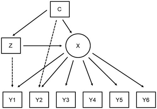
All three approaches, that is, the regression adjustment as well as the one-step and three-step IPW approaches, account for the scenario depicted in Figure 1 where the treatment effect Z on the latent Variable X is confounded by C. Note that in this setting, the observed indicators Y are unaffected by the treatment or the confounders conditional on the latent variable (local independence). That is, all differences in the observed indicators that are caused by either the treatment or the confounders are captured in the latent classes. While this is a crucial assumption when using latent class analysis, this is often not the case in reality (Masyn, 2017; Vermunt & Magidson, 2021a). As depicted in Figure 2, there are scenarios where not all these differences in the observed indicators are captured in the latent classes. Here, the treatment, (some or all of) the confounders, or both have direct effects on some of the observed indicators even after introducing the latent classes. This situation where auxiliary variables have direct effects on the observed indicators is also called measurement non-invariance (MNI) or differential item functioning (DIF; Masyn, 2017). In the remainder of this study, we will use the terms MNI and DIF interchangeably. As an example of DIF, let’s consider the study about college enrollment and substance use presented in Lanza et al. (2013). Substance use was assessed by self-reported drinking behavior, use of cigarettes, marijuana, and crack/cocaine, and two classes labeled by the authors as “low-level users” and “heavy drinkers” were identified. However, the “heavy drinker” class also showed higher levels of cigarette and marijuana use and could alternatively be labeled “higher-level users.” We re-analyzed this data following Lanza and colleagues’ analysis strategy and replicated a large ATE. Attending college leads to a higher probability of belonging to the low-level users’ class (87.7% vs. 51.4%) and to a lower probability of belonging to the higher-level users’ class (12.3% vs. 48.6%). Alternatively, the ATE could be expressed in an odds ratio of 0.15, meaning that if all individuals in the population were to attend college, the overall odds of membership in the low-level users’ class is 6.7 times more likely than if all individuals were not to attend college (Lanza et al., 2013). However, upon closer examination of the results, we identified high bivariate residuals (BVR) for college enrollment and some of the indicators that are signs for the presence of DIF (Vermunt & Magidson, 2021a). By not taking into account this DIF, the strength of the ATE in this example has been drastically overestimated. In essence, the measurement models for the two groups (college attendees and college non-attendees) are not identical and the estimation of the measurement model can therefore not be separated from the estimation of the structural model. To allow these differences in the measurement model, the direct effects of the auxiliary variables on the indicators need to be explicitly modeled in the measurement model (Vermunt & Magidson, 2021a). Both the one-step analysis strategy by Lanza et al. (2013) and the three-step analysis strategy by Clouth et al. (2022) do not account for these direct effects.

Figure 1. Latent class model with confounded treatment effect.

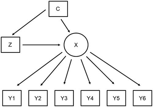
Figure 2. Latent class model with confounded treatment effect where both treatment and the confounders have direct effects on some observed indicators.

Consequences of not accounting for such direct effects are well established (Asparouhov & Muthén, 2014; Di Mari & Bakk, 2018; Janssen et al., 2019; Masyn, 2017; Vermunt & Magidson, 2021a). In short, these authors show that if a covariate has direct effects on (some) indicator variables and this is neglected, the effect of that covariate on the latent variable will be estimated with a bias. This bias depends on the effect size of the direct effects, the sample size, and on how many indicators a covariate has direct effects (Janssen et al., 2019). Vermunt and Magidson (2021a) find that mainly the estimate of the covariate with direct effects is biased, but covariates without direct effects seem to be unaffected even if other direct effects in the model are neglected. Direct effects can be directly included when the model is estimated in one step (Asparouhov & Muthén, 2014). However, when using the three-step approach, Vermunt and Magidson (2021a) show that some additional considerations need to be made. The three steps of their approach contain:

1. The measurement model is estimated including the direct effects and the effects of the covariate on the latent variable. Covariates without direct effect are not included in the model in this step.

2. The classifications are obtained as in a standard three-step LC model; however, because of the modified step one, they now also depend on the values of the covariates with direct effects.

3. In the last step, all covariates, that is, the covariates that were already included in step one and new covariates without direct effects, are included in the structural model. Crucially, this improved approach by Vermunt and Magidson (2021a) also allows the matrix containing the classification error corrections, also referred to as the D matrix, to differ over the values of the covariates with direct effects.

This article offers three main contributions to the existing literature.

• We propose an analysis strategy that extends the approach by Clouth et al. (2022) with the additional modeling steps proposed by Vermunt and Magidson (2021a) to correctly account for DIF.

• We present a strategy for detecting DIF caused by the treatment or confounding variables.

• We investigate the performance of our newly proposed analysis strategy when DIF is present in the data and compare it to the approaches by Lanza et al. (2013) and Clouth et al. (2022).

In the next section, we will formally derive latent class models that correctly incorporate direct effects when using the regression adjustment approach, the one-step IPW, and the three-step IPW approach. Next, we will demonstrate that ignoring these direct effects indeed causes a biased estimate of the ATE and investigate how the three approaches perform on simulated data. We will then re-analyze the data from the National Longitudinal Survey of Youth data set (Lanza et al., 2013) on substance use. We end with a discussion and conclusion section. All code used for the simulated data example and the real-life data example is available in the Appendix and on GitHub, https://github.com/felixclouth/LCA-with-IPW-in-the-presence-of-DIF.

2. The Latent Class Model with Treatment Effects

Figure 1 depicts a latent class model where class membership (the latent variable X) is explained by treatment Z, and this treatment effect is confounded by a set of confounders C. This model can be broken down into three parts.

First, the treatment allocation model $P\left(Z_i\right|{\mathit{C}}_{\mathit{i}})$ deals with the problem of confounding that occurs in observational data. $P\left(Z_i\right|{\mathit{C}}_{\mathit{i}})$ can be explicitly modeled, e.g., by means of logistic regression, and yields the propensity score. When properly specified, the propensity score (PS) entails all the information needed to solve the confounding problem, that is, the probability of receiving treatment conditional on the (measured) confounders (Austin, 2011). In consecutive analyses, the propensity score can be used as a control variable in a regression model, to perform matching, or to construct inverse propensity weights (Austin, 2011).

Second, the structural model $P\left(X\right|Z_i,{\mathit{C}}_{\mathit{i}})$ describes the relationship of treatment and the confounders with the latent variable X (Vermunt & Magidson, 2004). The probability of being classified into one of the latent classes is conditional on treatment and the confounders. It is the researcher’s choice how to model the average treatment effect ATE, i.e., the treatment effect conditional on the set of confounders $P\left(X\right|Z_i,{\mathit{C}}_{\mathit{i}})$ or the marginal treatment effect $P\left(X\right|Z_i)$ after performing matching or IPW (Austin, 2011). In fact, when estimating the conditional treatment effect, it is not necessary to explicitly model treatment allocation $P\left(Z_i\right|{\mathit{C}}_{\mathit{i}}).$

Third, the latent classes X affect the individual responses or observed indicators ${\mathit{Y}}_{\mathit{i}}$ through the measurement model $P\left({\mathit{Y}}_{\mathit{i}}\right|X).$ One crucial assumption of LCA is local independence, which states that the indicators ${\mathit{Y}}_{\mathit{i}}$ are conditional only on the latent classes X, implying that (1) the indicators are independent from each other conditional on X and (2), more importantly in this case, that the indicators are independent from treatment and the confounders conditional on X.

Combining these three parts, the full model can then be described as: (1) $$\begin{array}{c}P\left({\mathit{Y}}_{\mathit{i}},{X,Z}_i\right|{\mathit{C}}_{\mathit{i}})= P(Z_i\left|{\mathit{C}}_{\mathit{i}}\right) P\left(X\right|Z_i,{\mathit{C}}_{\mathit{i}}\left)P\right({\mathit{Y}}_{\mathit{i}}\left|X\right).\end{array}$$(1)

In the scenario depicted in Figure 2, DIF is caused by treatment and/or the confounders because they affect the indicators directly, that is, local independence does not hold anymore. This means that instead of measurement model $P\left({\mathit{Y}}_{\mathit{i}}\right|X)$ we have $P\left({\mathit{Y}}_{\mathit{i}}\right|X,Z_i),$ $P\left({\mathit{Y}}_{\mathit{i}}\right|X,{\mathit{C}}_{\mathit{i}}),$ or $P\left({\mathit{Y}}_{\mathit{i}}\right|X,{Z_i,\mathit{C}}_{\mathit{i}}).$ In the remainder of this study, we will focus on the case where DIF is caused by either the treatment or the confounders but not both. The specification of the full model then changes to: (2) $$\begin{array}{c}P\left({\mathit{Y}}_{\mathit{i}},{X,Z}_i\right|{\mathit{C}}_{\mathit{i}})= P(Z_i\left|{\mathit{C}}_{\mathit{i}}\right) P\left(X\right|Z_i,{\mathit{C}}_{\mathit{i}}\left)P\right({\mathit{Y}}_{\mathit{i}}\left|X,Z_i\right)\end{array}$$(2)

or (3) $$\begin{array}{c}P\left({\mathit{Y}}_{\mathit{i}},{X,Z}_i\right|{\mathit{C}}_{\mathit{i}})= P(Z_i\left|{\mathit{C}}_{\mathit{i}}\right) P\left(X\right|Z_i,{\mathit{C}}_{\mathit{i}}\left)P\right({\mathit{Y}}_{\mathit{i}}\left|X,{\mathit{C}}_{\mathit{i}}\right). \end{array}$$(3)

While solutions to estimate the model under Equation (1)(1) $$\begin{array}{c}P\left({\mathit{Y}}_{\mathit{i}},{X,Z}_i\right|{\mathit{C}}_{\mathit{i}})= P(Z_i\left|{\mathit{C}}_{\mathit{i}}\right) P\left(X\right|Z_i,{\mathit{C}}_{\mathit{i}}\left)P\right({\mathit{Y}}_{\mathit{i}}\left|X\right).\end{array}$$(1) (corresponding to Figure 1) have been previously proposed (Clouth et al., 2022; Lanza et al., 2013), so far, there is no solution on how to estimate Equation (2)(2) $$\begin{array}{c}P\left({\mathit{Y}}_{\mathit{i}},{X,Z}_i\right|{\mathit{C}}_{\mathit{i}})= P(Z_i\left|{\mathit{C}}_{\mathit{i}}\right) P\left(X\right|Z_i,{\mathit{C}}_{\mathit{i}}\left)P\right({\mathit{Y}}_{\mathit{i}}\left|X,Z_i\right)\end{array}$$(2) or Equation (3)(3) $$\begin{array}{c}P\left({\mathit{Y}}_{\mathit{i}},{X,Z}_i\right|{\mathit{C}}_{\mathit{i}})= P(Z_i\left|{\mathit{C}}_{\mathit{i}}\right) P\left(X\right|Z_i,{\mathit{C}}_{\mathit{i}}\left)P\right({\mathit{Y}}_{\mathit{i}}\left|X,{\mathit{C}}_{\mathit{i}}\right). \end{array}$$(3) (corresponding to Figure 2) in a causal inference setting. In the following section, we describe in detail how these models can be estimated using the regression adjustment approach, the one-step approach, and the three-step approach.

2.1. Approach 1: LC Analysis with Regression Adjustment

This approach combines the treatment-allocation model, the structural model, and the measurement model into one analysis. In fact, the treatment allocation model for $P\left(Z_i\right|{\mathit{C}}_{\mathit{i}})$ can be ignored, and both the treatment Z and the confounders C are included in the LC model directly as covariates. This results in estimating the joint probability of the indicators and latent class conditional on treatment and the confounders: (4) $$\begin{array}{c}P\left({\mathit{Y}}_{\mathit{i}},X\right|Z_i,{\mathit{C}}_{\mathit{i}})= P(X\left|Z_i,{\mathit{C}}_{\mathit{i}}\right)P\left({\mathit{Y}}_{\mathit{i}}\right|X). \end{array}$$(4)

Measurement non-invariance is dealt with by including the direct effects of confounders and/or treatment in the model, which involves replacing $P\left({\mathit{Y}}_{\mathit{i}}\right|X)$ by $P\left({\mathit{Y}}_{\mathit{i}}\right|X,{\mathit{C}}_{\mathit{i}})$ or $P\left({\mathit{Y}}_{\mathit{i}}\right|X,Z_i).$

For detecting DIF, the correct model-building strategy is crucial. As shown by Nylund-Gibson and Masyn (2016), model selection should be performed on the measurement model without including any covariates to prevent the risk of overestimating the number of classes. Note that this step might involve relaxing the assumption of local independence by including direct effects between the indicators. After selecting the correct measurement model, the model should be re-estimated with the treatment variable and the confounders included in the model. Next, local dependencies between the auxiliary variables and the indicators need to be detected. This can be done using score tests or by inspecting the bivariate residuals (BVR;(Masyn, 2017; Oberski et al., 2013; Visser & Depaoli, 2022). These local dependencies should be addressed step by step by including direct effects until settling on a final model that does not show high bivariate residuals anymore.

2.2. Approach 2: One-Step LC Analysis with IPWs

With this approach, first proposed by Lanza and colleagues (Lanza et al., 2013), the treatment-allocation problem is dealt with separately, while the structural model and the measurement model are estimated simultaneously. $P\left(Z_i\right|{\mathit{C}}_{\mathit{i}})$ can be estimated in various ways but logit and probit regression are widely used choices. The advantage of the propensity score (typically denoted as $\pi$) is that it combines all the information provided by the (measured) confounders into one single score, which easily facilitates successive analyses (Austin, 2011). For instance, weights based on the inverse of the propensity score can be constructed. To estimate the ATE for the entire population, weights for IPW are constructed as ${\mathit{ipw}}_i=1/{\widehat{\pi }}_i$ for individuals that received treatment and ${\mathit{ipw}}_i=1/(1-{\widehat{\pi }}_i)$ for individuals that did not receive treatment (Austin, 2011). However, alternative weights to estimate the treatment effect among the treated (ATT) are also possible. IPW is used to achieve balance on the measured confounders at baseline between the treatment group and the control group. With this balancing property we generate a synthetic data set that emulates data from a randomized controlled trial and, therefore, allow for the estimation of causal marginal treatment effects (Austin, 2011). Note that, for a valid causal interpretation of the ATE, important assumptions need to be met that are discussed elsewhere (Hernán & Robins, 2006).

Next, the LC model for $P\left({\mathit{Y}}_{\mathit{i}},X\right|Z_i)$—thus, excluding the confounders—can be estimated on the balanced data set (Lanza et al., 2013). The LC model has the following form: (5) $$\begin{array}{c}P\left({\mathit{Y}}_{\mathit{i}},X\right|Z_i)= P(X\left|Z_i\right)P\left({\mathit{Y}}_{\mathit{i}}\right|X). \end{array}$$(5)

While the confounders ${\mathit{C}}_{\mathit{i}}$ do not appear anymore in Equation (5)(5) $$\begin{array}{c}P\left({\mathit{Y}}_{\mathit{i}},X\right|Z_i)= P(X\left|Z_i\right)P\left({\mathit{Y}}_{\mathit{i}}\right|X). \end{array}$$(5) , they are controlled for through the weighting. Note that this approach easily facilitates the use of other causal inference techniques to estimate the marginal treatment effect such as matching or stratification.

In case of DIF related to treatment, we can include direct effects of treatment in the LC measurement model, that is, replace $P\left({\mathit{Y}}_{\mathit{i}}\right|X)$ by $P\left({\mathit{Y}}_{\mathit{i}}\right|X,Z).$ However, it is unclear how to deal with DIF related to confounders because they do not appear in the estimated-LC model. It is possible to include only the covariates related to DIF in the LC model; however, it is unclear if these confounders should then also be included in the propensity-score model. In case they would be included, this would, in fact, relate to a situation similar to estimating (partly) doubly robust estimators (Robins et al., 1994). However, such an analysis strategy has not been investigated before and it is unclear how this approach would perform.

2.3. Approach 3: Three-Step LC Analysis with IPWs

Here, the treatment-allocation problem, the structural model, and the measurement model are dealt with separately (Clouth et al., 2022). The propensity-score model and the construction of the weights are done exactly the same way as in approach 2.

In a first step, an LC model for $P\left(X,{\mathit{Y}}_{\mathit{i}}\right)$ is estimated on the original, unweighted data: (6) $$\begin{array}{c}P\left(X,{\mathit{Y}}_{\mathit{i}}\right)= P\left(X\right)P\left({\mathit{Y}}_{\mathit{i}}\right|X).\end{array}$$(6)

To estimate the measurement model without the inclusion of covariates or weighting has several conceptual advantages regarding interpretation or class enumeration that are discussed in more detail, amongst others, by Clouth et al. (2022), Nylund-Gibson et al. (2014), and Vermunt (2010). In a second step, class assignments $W_i$ are obtained either using modal assignment, that is, the individual is assigned to the class for which their posterior class membership probabilities $P(X|{\mathit{Y}}_{\mathit{i}})$ are highest, or proportional assignment, that is, a soft partitioning where $W_i$ equals $P(X|{\mathit{Y}}_{\mathit{i}})$ for each respective class. Additionally, the classification errors $P\left(W_i\right|X)$ are computed (Vermunt, 2010). Step three in this approach involves estimating a model for $P\left(X,W_i\right|Z_i)$ using the IPWs based on $P\left(Z_i\right|{\mathit{C}}_{\mathit{i}})$ as weights while accounting for the fact that the class assignments $W_i$ contain classification errors using $P\left(W_i\right|X)$ as fixed probabilities (Clouth et al., 2022). This third-step structural model has the following form: (7) $$\begin{array}{c}P\left(X,W_i\right|Z_i)=P(X\left|Z_i\right)P\left(W_i\right|X). \end{array}$$(7)

For DIF caused by treatment we can make use of the work by Vermunt and Magidson (2021a). Key is that the variable causing DIF, here the treatment, should be included in the step one model; that is, we specify a model for $P\left(X,{\mathit{Y}}_{\mathit{i}}\right|Z_i)$ with $P\left({\mathit{Y}}_{\mathit{i}}\right|X)$ replaced by $P\left({\mathit{Y}}_{\mathit{i}}\right|X,Z_i).$ As shown by Vermunt and Magidson (2021a), crucially, also the classification errors $P\left(W_i\right|X)$—sometimes referred to as the D-matrix—now depend on treatment, resulting in $P\left(W_i\right|{X,Z}_i).$ The third step again consists of estimating Equation (7)(7) $$\begin{array}{c}P\left(X,W_i\right|Z_i)=P(X\left|Z_i\right)P\left(W_i\right|X). \end{array}$$(7) on the weighted data where $P\left(W_i\right|X)$ is substituted for $P\left(W_i\right|{X,Z}_i).$ The same problem as described in approach two appears if DIF is related to the confounders. Theoretically, it is possible to include ${\mathit{C}}_{\mathit{i}}$ in the first step and obtain classification errors $P\left(W_i\right|{X,\mathit{C}}_{\mathit{i}}).$¹ However, if these confounders are also included in the propensity-score model, the ATE is essentially estimated by a partly doubly robust method with unknown properties.

3. A Demonstration Using a Simulated Data Example

For this demonstration, we simulated one synthetic data set for each condition that is exactly in agreement with the population. This can be done using the “write exemplary” option in Latent Gold 6.0 (Vermunt & Magidson, 2021b). Our data-generating models closely resemble the setting in Vermunt and Magidson (2021a) and are similar to the one depicted in Figure 2. We investigated the bias of the ATE for the regression adjustment method, the one-step IPW method, and the three-step IPW method (1) when the direct effects are ignored and (2) when the direct effects are correctly modeled as illustrated above.

3.1. Method

In detail, the true model consists of three latent classes, six dichotomous indicators (high/low), one treatment variable Z (0 = control, 1 = treatment), and two categorical confounders (–.5; .5 for C₁ and −2; −1; 0; 1; 2 for C₂). In class 1, the item response probabilities for a high response were 0.8 for all items; in class 2, these probabilities were 0.8 for the first three items and 0.2 for the last three items; and in class 3, they were 0.2 for all items. This setup resembles moderate class separation and was also used by Vermunt (2010) and Clouth et al. (2022). These probabilities for a high response correspond to logit values of 1.3863 and −1.3863, respectively. The covariate effects on the classes were modeled using multivariate logistic regression with class 1 as the reference class and logit parameters of [–1, −1, 1, 1] (including the first parameter for the intercept) for class 2 and [–2, 1, −1, ${\gamma }_Z$] for class 3 where ${\gamma }_Z$ was varied with [1, 2] for the effect of treatment. The effect of the confounders on the treatment assignment, thus, the propensity-score model, was modeled using binary logistic regression with logit parameters of [0, ${\beta }_1,$ 1] with ${\beta }_1$ [1, 2]. Furthermore, there are two main scenarios to be considered. In scenario 1, Z has direct effects on the indicators three and six and in scenario 2, C₁ has direct effects on the indicators three and six with the logits for these direct effects set to 1. Table 1 gives an overview of the resulting scenarios from varying these parameters.

Table 1. Bias of the estimate of the ATE.

DIF variable	Z				C1
${\gamma }_Z$	1		2		1		2
${\beta }_1$	1	2	1	2	1	2	1	2
Regression adjusted	0.069	0.068	0.049	0.050	–0.002	–0.003	–0.003	–0.004
One-step IPW	0.073	0.073	0.049	0.049	–0.001	–0.001	–0.002	–0.002
Three-step IPW	0.066	0.065	0.054	0.054	–0.001	–0.001	–0.003	–0.002
Regression adjusted with DIF	0.000	0.000	0.000	0.000	0.000	0.000	0.000	0.000
One-step IPW with DIF	0.000	0.000	0.000	0.000	0.000	0.000	0.000	0.000
Three-step IPW with DIF	0.000	0.000	0.000	0.000	0.000	0.000	–0.001	–0.001

Note. These results are based on the analysis of synthetic data sets that were generated to be exactly in agreement with the population values. The data sets resemble a sample size of 1,000.

Generally, it is up to the researcher to define the ATE when using LCA in this context. For instance, there might be a class for which class membership might be unfavorable, such as a poor quality of life class or a high substance-use class. The ATE can then be defined as the difference in class membership probability under treatment option A compared to treatment option B for the unfavorable class concerned.² In our simulated data example, we arbitrarily chose to define the ATE to be the difference in class membership probability for class three.

3.2. Results

Table 1 reports the bias of the estimate of the ATE for the regression adjustment approach, the one-step IPW approach, and the three-step IPW approach where for all approaches direct effects have either been ignored or correctly modeled. Results are presented for varying levels of effect sizes for the true ATE and the true confounding effect where either treatment or a confounding variable causes DIF. As can be seen, all three approaches reproduce the true ATE perfectly when direct effects are modeled correctly. When DIF is ignored, all three approaches estimate the ATE with a severe bias if treatment has the direct effects on the indicators. The bias decreases for stronger effects of the treatment on the classes but is unaffected by the strength of confounding. Here, the parameters were overestimated. However, the direction of the bias depends on the direction of the direct effects and on which classes are compared. If DIF is caused by a confounding variable, the ATE seems to be mostly unaffected even when DIF is ignored.

4. A Real-Life Example Using Data from the National Longitudinal Survey of Youth 1979

In this example, we re-analyze data from the National Longitudinal Survey of Youth 1979 (NLSY79) that was used as a motivating example by Lanza et al. (2013). The NLSY79 cohort is a representative sample of the American youth born between 1957 and 1964. Annual interviews were conducted between 1979 and 1994 (Center for Human Resource Research, 1997).

Lanza et al. (2013) investigated substance use by a sample of participants that was approximately 33 years old in 1994. They used LCA to construct classes of substance use indicated by drinking behavior, smoking, use of marijuana, and use of crack/cocaine. Furthermore, they investigated the effect of college attendance on class membership, hypothesizing that college attendance serves as a protective measure against substance use at a later stage of life. The analysis was adjusted for factors related to selection effects of college enrollment using IPW. These confounding variables were measured in the first round in 1979, one year before potential college enrollment.

4.1. Method

In detail, identified as confounding variables were gender, race/ethnicity, household income, if the household was a single-parent household, residential crowding, years of maternal education, maternal age, metropolitan status, the language spoken at home, educational aspirations of the adolescent and the parent(s), and type of high school (vocational, commercial, general program, college preparatory; Lanza et al., 2013). One year later in round two, full-time college enrollment was assessed. Finally, in round 16 (1994), substance use was assessed. Drinking behavior was coded with “0” representing “no use in the past month,” “1” representing “alcohol use but no binge drinking in the last month,” and “2” representing “binge drinking, having six or more drinks at one time in the last month.” Cigarette use, marijuana use, and a composite item of either crack or cocaine use were coded as “0” reflecting “no use” and “1” reflecting “any use.”

In the following list, we describe step by step the analysis strategy we followed.

1. Model selection for the measurement model. First, we estimated an LC model based on the four indicators alcohol use, cigarette use, marijuana use, and crack or cocaine use. The BIC indicated that a two-class model fits the data best. However, as indicated by a large bivariate residual (BVR), there was still a local dependency between the indicators marijuana use and crack/cocaine use. Instead of choosing a three-class model for which no local dependencies could be detected, we chose to select the two-class model while allowing for this local dependency. We believe that this was not done by Lanza et al. (2013). Our results (Table 2) are therefore not directly comparable; however, our classes still have the same interpretation with class 1 being a no-to-low usage class and class 2 being a heavy usage/heavy drinker class.

2. Detecting DIF. Next, we re-estimated this LC model including college attendance as our treatment in the model (one-step LCA). This is primarily done to check if there are local dependencies between our treatment variable and the indicators (as indicated by large BVRs). Such local dependencies would indicate DIF thus, that not all of the effect of the treatment on the observed indicators goes through the latent classes. Note that the parameter estimate of treatment in this step does not reflect the ATE and is therefore not of interest because confounding is not (yet) accounted for. In our example, two dependencies, college–alcohol use and college–cigarette use, were detected. We re-estimated the LC model including these dependencies and saved the classifications and posterior class-membership probabilities. Note that in this step also local dependencies between indicator variables can show. While dependencies are introduced by the treatment variable, the maximum likelihood solution only picks up that there are dependencies in the model and allocates them in a sort of tradeoff between dependencies between the treatment and the indicators and between the indicators themselves. However, because we already accounted for local dependencies between indicators in step one, we know that accounting for the dependencies between the treatment and the indicators will also diminish the detected dependencies between the indicator variables.³

3. Multiple imputation. In this step, missing values on the confounders were imputed. We conducted multiple imputation using the MICE package in R (Van Buuren & Groothuis-Oudshoorn, 2011). Note that, again, this step is slightly different to the analysis by Lanza et al. (2013). For this multiple imputation step, two open questions remain. First, should college attendance as our treatment variable be imputed because it functions as both, a dependent variable (in the propensity score model) and an independent variable (when estimating the ATE)? Here, we chose to impute college attendance to keep the same sample size as in Lanza and colleagues. Second, it is unknown if the indicator variables, the class assignments, or both should be included as predictors for imputation. Here, we included the observed indicators.

4. Propensity scores and IPW. After imputing missing values, the model for the propensity scores can be estimated. We used logistic regression with college attendance as outcome and before-mentioned confounders as predictor variables. After obtaining the propensity scores ${\widehat{\pi }}_i,$ the weights were constructed using the inverse of the propensity scores, that is, $1/{\widehat{\pi }}_i$ for individuals who received the treatment and $1/1-{\widehat{\pi }}_i$ for individuals who did not receive the treatment. Additionally, manipulations to the weights, such as truncating or construction of stabilized weights (Robins et al., 2000), can be performed in this step. Furthermore, the use of IPW requires checking several assumptions that are needed for causal inference (Hernán & Robins, 2006). In this example, there was sufficient overlap of the propensity scores (see Figure 3) and weighting achieved good balance (see Table 3) between the treatment and non-treatment group as indicated by standardized mean differences (SDM) <.2 and p-values <.05 (Austin, 2009). Note that all steps described here have to be done for each imputed data set separately.

5. Estimating the ATE. In the last step, the classifications and classification errors obtained in step two are used in the third step of a bias-adjusted three-step LCA (Vermunt, 2010) to estimate the ATE, and thus, the effect of college attendance on the classes weighted with the IPW (i.e., see Equation (7)(7) $$\begin{array}{c}P\left(X,W_i\right|Z_i)=P(X\left|Z_i\right)P\left(W_i\right|X). \end{array}$$(7) ). Importantly, the correction for the classification errors that serve as a weight in the three-step LCA need to be allowed to vary between treatment groups (Vermunt & Magidson, 2021a). This fifth step is performed separately for each imputed data set and results are pooled using Rubin’s rule.

Figure 3. Overlap of the propensity scores.

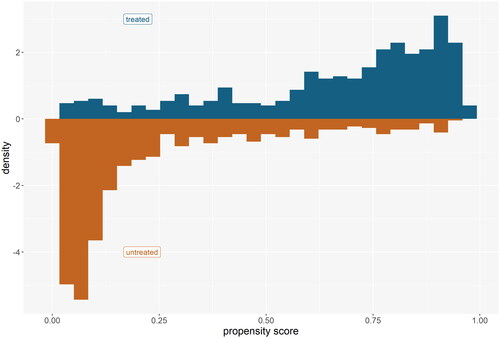
Table 2. Profiles of the two identified classes.

	Lanza et al.		Three-step
	Class 1	Class 2	Class 1	Class 2
	0.70	0.30	0.68	0.32
Alcohol
No use	0.57	0.18	0.55	0.05
Light use	0.29	0.35	0.38	0.33
Binge	0.14	0.47	0.07	0.62
Cigarette
No use	0.91	0.47	0.82	0.53
Use	0.09	0.53	0.18	0.47
Marijuana
No use	0.99	0.83	0.99	0.79
Use	0.01	0.17	0.01	0.21
Crack/Cocaine
No use	1.00	0.94	1.00	0.95
Use	0.00	0.06	0.00	0.05

Note. These parameter estimates result from estimating the first step, i.e., the measurement model without the inclusion of covariates. Note that the first step of the three-step analysis includes direct effects between college-alcohol use and college-cigarette use, while the analysis by Lanza et al. (2013) does not.

Table 3. Balance of the college enrolled vs. not enrolled group before and after IPW.

	No weights				Inverse propensity weights
	Not enrolled	Enrolled	p-value	SMD	Not enrolled	Enrolled	p-value	SMD
N	651	441			1086.3	1119.9
Age (mean, SD)	17.7 (0.8)	17.4 (0.6)	<0.001	0.415	17.6 (0.7)	17.6 (0.8)	0.578	0.078
Gender (female)	312 (47.9%)	247 (56.0%)	0.009	0.162	545.8 (50.2%)	543.8 (48.6%)	0.746	0.034
Race			0.048	0.154			0.623	0.101
White	413 (63.4%)	310 (70.3%)			677.3 (62.4%)	642.7 (57.4%)
Black	210 (32.3%)	119 (27.0%)			365.8 (33.7%)	427.8 (38.2%)
Other	28 (4.3%)	12 (2.7%)			43.1 (4.0%)	49.4 (4.4%)
Household income (mean, SD)	16055 (11323)	22855 (15214)	<0.001	0.507	17661 (11868)	18116 (13185)	0.695	0.036
Nr. siblings			<0.001	0.416			0.948	0.222
0	19 (2.9%)	12 (2.7%)			30.0 (2.8%)	24.3 (2.2%)
1	62 (9.5%)	87 (19.7%)			136.6 (12.6%)	165.4 (14.8%)
2	121 (8.6%)	109 (24.7%)			235.6 (21.7%)	230.7 (20.6%)
3	155 (23.8%)	78 (17.7%)			248.9 (22.9%)	253.5 (22.6%)
4	88 (13.5%)	56 (12.7%)			134.0 (12.3%)	96.6 (8.6%)
5	68 (10.4%)	37 (8.4%)			95.5 (8.8%)	115.7 (10.3%)
6 or more	138 (21.2%)	62 (14.0%)			205.9 (18.9%)	233.6 (21.0%)
Language			0.911	0.027			0.186	0.216
English	538 (82.6%)	360 (81.6%)			865.0 (79.6%)	828.2 (74.0%)
Spanish	80 (12.3%)	57 (12.9%)			150.6 (13.9%)	147.9 (13.2%)
Other	33 (5.1%)	24 (5.4%)			70.7 (6.5%)	143.7 (12.8%)
Maternal education (mean, SD)	10.5 (2.8)	11.9 (3.1)	<0.001	0.491	11.1 (2.9)	11.07 (3.34)	0.970	0.004
Education aspiration years (mean, SD)	13.2 (1.7)	15.7 (1.6)	<0.001	1.578	14.1 (2.1)	14.2 (2.0)	0.795	0.029
Education aspiration (yes)	138 (21.2%)	205 (46.5%)	<0.001	0.555	365.0 (33.6%)	440.1 (39.3%)	0.284	0.119
Parent figure (both)	512 (78.6%)	387 (87.8%)	<0.001	0.245	868.9 (80.0%)	841.9 (75.2%)	0.364	0.115
Metropolitan status (urban)	478 (73.4%)	367 (83.2%)	<0.001	0.239	852.1 (78.4%)	924.3 (82.5%)	0.260	0.103
College preparation program			<0.001	0.817			0.924	0.065
Vocational	161 (24.7%)	44 (10.0%)			202.8 (18.7%)	204.3 (18.2%)
Commercial	21 (3.2%)	15 (3.4%)			30.1 (2.8%)	34.6 (3.1%)
College preparatory	122 (18.7%)	239 (54.2%)			358.6 (33.0%)	400.3 (35.7%)
General program	347 (53.3%)	143 (32.4%)			494.7 (45.5%)	480.7 (42.9%)

Note. SMD <0.2 and p-values > 0.05 indicate good balance between the groups.

4.2. Results

The results of this last step are presented in Table 4. Attending college leads to a reduced probability of class membership in the high-usage class (0.25 [0.21; 0.30] vs. 0.35 [0.33; 0.36]; ATE = −0.09 [–0.14; −0.04]). Alternatively, the ATE can be expressed as an OR of 0.64 [0.49; 0.83]. Consequently, if all individuals attended college, the overall odds of class membership in the high-usage class would be 1.56 times higher than if all individuals did not attend college. Parameter estimates for the direct effects of college attendance on alcohol use and cigarette use are reported in Tables 5 and 6, respectively. Comparing these results to the OR of 0.15 [0.11; 0.20] reproduced from Lanza et al. (2013), the strength of the ATE seems to be drastically overestimated when not accounting for DIF.

Table 4. Class membership probabilities estimated in the last step of our newly proposed analysis strategy.

College	Class 1	Class 2
No	0.65	0.35
Yes	0.75	0.25

Note. The ATE can be depicted in an odds ratio of 0.64 compared to an odds ratio of 0.16 reported by Lanza et al. (2013).

Table 5. Direct effects between college and alcohol use.

		Alcohol
College		No use	Light use	Binge
No	Class 1	0.60	0.33	0.08
No	Class 2	0.05	0.28	0.66
Yes	Class 1	0.50	0.44	0.06
Yes	Class 2	0.05	0.40	0.55

Note. These direct effects are estimated without weighting in our proposed analysis strategy.

Table 6. Conditional response probabilities for cigarette use per treatment group.

		Cigarette
College		No use	Use
No	Class 1	0.77	0.23
No	Class 2	0.45	0.55
Yes	Class 1	0.90	0.10
Yes	Class 2	0.68	0.32

Note. These direct effects are estimated without weighting in our proposed analysis strategy.

In addition to this analysis, we followed the analysis strategy proposed by Lanza et al. (2013) while also accounting for direct effects. For this, we first performed multiple imputation to estimate the propensity-score model. For each imputed set, we followed with conducting the weighting and estimating the LC model without college attendance. Before including the treatment variable in the model, we allowed for direct effects to account for dependencies between the indicator variables. After settling on the final measurement model, we included college attendance in the model and allowed for direct effects between college attendance and indicator variables where local dependencies showed. Eventually, results were pooled over the imputed sets. Results for the ATE are presented in Table 7 and the direct effects between college–cigarette use and college–marijuana use are presented in Table 8. With an OR of 0.44 [0.35; 0.51], the ATE is estimated to be a bit stronger than following the three-step approach. However, it still clearly shows that the strength of the ATE is overestimated when direct effects are not accounted for.

Table 7. Class membership probabilities estimated with the modified analysis strategy based on Lanza et al. (2013).

College	Class 1	Class 2
No	0.58	0.42
Yes	0.76	0.24

Note. The ATE can be depicted in an odds ratio of 0.44.

Table 8. Conditional response probabilities for cigarette use, marijuana use, and crack/cocaine use estimated using the modified analysis strategy based on Lanza et al. (2013).

		Cigarette
		No use				Use
		Marijuana
		No use		Use		No use		Use
		Crack/Cocaine
College		No use	Use	No use	Use	No use	Use	No use	Use
No	Class 1	0.74	0.00	0.00	0.00	0.25	0.00	0.00	0.00
No	Class 2	0.45	0.01	0.08	0.01	0.36	0.02	0.06	0.02
Yes	Class 1	0.90	0.00	0.00	0.00	0.09	0.00	0.00	0.00
Yes	Class 2	0.66	0.01	0.12	0.01	0.16	0.01	0.03	0.01

Note that there is an important difference in the direct effects between college attendance and the indicators in this modified one-step approach compared to our three-step approach. While in the modified one-step approach these direct effects are estimated on a weighted data set, they are estimated on an unweighted data set in the three-step approach. Because of this, the three-step approach does not allow for the inclusion of these direct effects in the definition of the ATE.

5. Discussion

In this article, we present an analysis strategy and a modification to the three-step LCA with IPW (Clouth et al., 2022) to correctly account for the scenario where a treatment or exposure causes DIF. When there is DIF caused by the treatment variable and the direct effects on the indicators are not modeled, the ATE estimates will be biased. However, results from the simulated data example also showed that DIF caused by the confounding variables does not affect the estimate of the ATE. This is an important finding because there is often a large number of confounders, and detecting and modeling each direct effect can be tedious or even infeasible.

The examples presented in this article also highlight the importance of a correct model-building strategy. First, we construct the correct measurement model, where class enumeration is done on a model including only the indicators, and potential local dependencies among indicators are modeled by direct effects between these indicators. Crucially, the final measurement model stays untouched in the consecutive steps. This prevents the detection of spurious classes due to dependencies introduced by auxiliary variables and allows for the interpretation of the classes based on the indicators only. Next, the treatment variable is included in this one-step model to detect DIF, which can be done by inspecting the residual associations (e.g., the BVRs). This step can be confusing because there might not only be high BVRs for the treatment and indicator variables but also between the indicators themselves. Note, however, that the correct measurement model has already been selected in the first step. Therefore, all dependencies that show in this step can be removed by introducing direct effects between the treatment and the indicators only. The third step now consists of re-estimating the structural model using IPW. As shown by Vermunt and Magidson (2021a), it is crucial that the matrix containing the classification-error corrections (D Matrix) is now allowed to vary over values of the treatment variable. This analysis strategy differs from the approach used in Lanza et al. (2013) and our modification of their approach, resulting in different measurement models. Consequently, the difference in ATEs resulting from these approaches do not reflect differences in the effect of treatment on the latent variable but differences in the measurement model, and thus, differences in the construction of the latent variable.

The difference of these results highlights the importance of explicitly defining the ATE. When accounting for DIF as proposed here, there are not only effects of the treatment on class membership but also the direct effects on indicators. We do not regard these direct effects as ATEs because they only reflect the fact that the meaning of certain indicators is different across treated and non-treated. That is, we are interested in the effect of treatment on what the indicators have in common. In certain cases, however, one might want to treat these direct effects as additional ATEs. If this can be done is a rather conceptual question and is probably related to the status of the indicators. That is, are these arbitrary indicators that could be replaced by other indicators to define the latent construct? Or are they rather specific indicators and the goal is to predict them, preferably via the classes for parsimony but if not possible, partially also through direct effects? Note that, regardless of the definition of the ATE, DIF always needs to be accounted for when present because the estimate of the ATE will otherwise be biased. Unfortunately, testing for DIF seems to be an uncommon practice (D’Urso et al., 2022).

There are some limitations to our study worth mentioning. The propensity-score model was specified perfectly in our simulated data example. However, for real-life data, the propensity-score model will likely be mis-specified to some extent. E.g., there might be unobserved confounding or the functional form of the model might be mis-specified because quadradic terms or interaction effects are not accounted for. How a mis-specified propensity-score model affects the estimate of the ATE for latent outcome classes is unknown and further research is needed. Furthermore, we only considered uniform DIF in this analysis. It is possible that, even after accounting for uniform DIF as done in this analysis, not all local dependencies are accounted for. In this case, it might be necessary to consider nonuniform DIF and allow the direct effects to vary between the latent classes. Lastly, we did not consider the problem of missing values. As shown by Alagöz and Vermunt (2022), if missing values of the indicators depend on values of auxiliary variables, the missing-values mechanism is missing at random in a one-step analysis but becomes missing not at random in a three-step analysis. In this situation, parameter estimates can be biased, which will likely also affect the analysis strategy proposed in this study.

Because the presented stepwise approach is particularly practical when resampling methods are being used, possible future extension of this work could investigate the use of multiple imputation for missing data or the use of the g-formula for time-varying treatment or causal mediation analysis.

6. Concluding Remarks

In this article, we propose a new analysis strategy to estimate ATEs for latent outcome classes in the presence of DIF. We extended previous work by Lanza et al. (2013) and Clouth et al. (2022) by incorporating the modified analysis steps proposed by Vermunt and Magidson (2021a) to correctly account for DIF. DIF caused by the confounding variables seems to not affect the ATE. However, when DIF caused by the treatment variable is not accounted for, the estimate of the ATE will be biased. As has been shown, this can be prevented by following the correct model-building strategy.

Acknowledgements

We would like to thank Dr. Stephanie Lanza for making code available to us facilitating the replication of the results in Lanza et al. (2013).

Disclosure Statement

No potential conflict of interest was reported by the author(s).

Additional information

Funding

This work was funded by The Netherlands Organisation for Scientific Research (NWO), Grant 628.001.030, “Helping cancer patients to choose the best treatment: Data-driven shared decisionmaking on cancer treatment for individual patients”.

Notes

1 The classification errors should only depend on C if C is also included as a covariate in step three. However, it is unclear if this is necessary or if after including C in step one and in the propensity model, step three should be estimated excluding C.

2 Alternatively, the ATE could be defined as a risk ratio or odds ratio.

3 We trust our simulation results that DIF of the confounders does not affect the estimate of the ATE substantially. Therefore, we do not check for local dependencies between the confounders and the indicators. While this could be done in this step, it quickly becomes infeasible with a larger number of confounders.

Appendix

Latent GOLD syntax for our newly proposed three-step IPW method accounting for DIF caused by the treatment as used in the real-life data example. The full code including the estimation of the propensity score model is available on GitHub.

Measurement model:

model

title FinalMeasurementModel;

options

maxthreads = all;

algorithm

 tolerance = 1e-008 emtolerance = 0.01 emiterations = 250 nriterations = 50;

startvalues

 seed = 0 sets = 16 tolerance = 1e-005 iterations = 50;

bayes

 categorical = 1 variances = 1 latent = 1 poisson = 1;

montecarlo

 seed = 0 sets = 0 replicates = 500 tolerance = 1e-008;

quadrature nodes = 10;

missing includeall;

output

 parameters = effect betaopts = wl standarderrors profile probmeans = posterior

 loadings bivariateresiduals estimatedvalues = model reorderclasses marchi2;

outfile “FinalMeasurementModel.sav”

 classification = posterior  keep id, Age, Gender, Race_ethnicity, Household_income,

  Number_Sib, Language_home, Maternal_education, Education_aspiration_1,

  Education_aspiration_2, Parent_figure, Metropolitan_status, College_Prep,

  Cigarette, Cocaine, Crack, PS, IPW;

variables

imputationid imp;

dependent Alcohol nominal, CigaretteDummy nominal, Marijuana nominal,

 CrackCocaine nominal;

independent college_enroll nominal;

latent

 Cluster nominal 2;

equations

Cluster <- 1 + college_enroll;

Alcohol <- 1 + Cluster + college_enroll;

CigaretteDummy <- 1 + Cluster + college_enroll;

Marijuana <- 1 + Cluster;

CrackCocaine <- 1 + Cluster;

Marijuana <-> CrackCocaine;

end model

Structural model:

model

title FinalStructuralModel;

options

maxthreads = all;

algorithm

 tolerance = 1e-008 emtolerance = 0.01 emiterations = 250 nriterations = 50;

startvalues

 seed = 0 sets = 16 tolerance = 1e-005 iterations = 50;

bayes

 categorical = 1 variances = 1 latent = 1 poisson = 1;

montecarlo

 seed = 0 sets = 0 replicates = 500 tolerance = 1e-008;

quadrature nodes = 10;

missing includeall;

step3 modal ml;

output

 parameters = first betaopts = wl standarderrors = robust profile = posterior

 probmeans = posterior estimatedvalues = model reorderclasses marginaleffects;

variables

imputationid imp;

samplingweight IPW rescale ipw;

independent college_enroll nominal;

latent Cluster nominal posterior = (Cluster#1 Cluster#2) dif = college_enroll;

equations

Cluster <- 1 + college_enroll;

end model.

References

- Alagöz, Ö. E. C., & Vermunt, J. K. (2022). Stepwise latent class analysis in the presence of missing values on the class indicators. Structural Equation Modeling, 29, 784–790. https://doi.org/10.1080/10705511.2022.2030743
- Asparouhov, T., & Muthén, B. (2014). Auxiliary variables in mixture modeling: Three-step approaches using Mplus. Structural Equation Modeling, 21, 329–341. https://doi.org/10.1080/10705511.2014.915181
- Austin, P. C. (2009). Balance diagnostics for comparing the distribution of baseline covariates between treatment groups in propensity-score matched samples. Statistics in Medicine, 28, 3083–3107. https://doi.org/10.1002/sim.3697
- Austin, P. C. (2011). An introduction to propensity score methods for reducing the effects of confounding in observational studies. Multivariate Behavioral Research, 46, 399–424. https://doi.org/10.1080/00273171.2011.568786
- Bakk, Z., & Vermunt, J. K. (2016). Robustness of stepwise latent class modeling with continuous distal outcomes. Structural Equation Modeling, 23, 20–31. https://doi.org/10.1080/10705511.2014.955104
- Bartolucci, F., Pennoni, F., & Vittadini, G. (2016). Causal Latent Markov Model for the comparison of multiple treatments in observational longitudinal studies. Journal of Educational and Behavioral Statistics, 41, 146–179. https://doi.org/10.3102/1076998615622234
- Bolck, A., Croon, M., & Hagenaars, J. (2004). Estimating latent structure models with categorical variables: One-step versus three-step estimators. Political Analysis, 12, 3–27. https://doi.org/10.1093/pan/mph001
- Bray, B. C., Dziak, J. J., Patrick, M. E., & Lanza, S. T. (2019). Inverse propensity score weighting with a latent class exposure: Estimating the causal effect of reported reasons for alcohol use on problem alcohol use 16 years later. Prevention Science, 20, 394–406. https://doi.org/10.1007/s11121-018-0883-8
- Center for Human Resource Research. (1997). National Longitudinal Survey of Youth (1997). Center for Human Resource Research.
- Clouth, F. J., Moncada-Torres, A., Geleijnse, G., Mols, F., van Erning, F. N., de Hingh, I. H. J. T., Pauws, S. C., van de Poll-Franse, L. V., & Vermunt, J. K. (2021). Heterogeneity in quality of life of long-term colon cancer survivors: A Latent Class analysis of the population-based PROFILES Registry. The Oncologist, 26, e492–e499. https://doi.org/10.1002/onco.13655
- Clouth, F. J., Pauws, S., Mols, F., & Vermunt, J. K. (2022). A new three-step method for using inverse propensity weighting with latent class analysis. Advances in Data Analysis and Classification, 16, 351–371. https://doi.org/10.1007/s11634-021-00456-5
- Collins, L. M., & Lanza, S. T. (2010). Latent class and latent transition analysis: With applications in the social, behavioral, and health sciences. Wiley.
- D’Urso, E. D., Maassen, E., Van Assen, M. A. L. M., Nuijten, M. B., De Roover, K., Wicherts, J. M. (2022). The Dire Disregard of measurement invariance testing in psychological science. PsyArXiv. https://osf.io/j72t4/?view_only=83cf802a792543419841d36cc885c702.
- Di Mari, R., & Bakk, Z. (2018). Mostly harmless direct effects: A comparison of different latent markov modeling approaches. Structural Equation Modeling, 25, 467–483. https://doi.org/10.1080/10705511.2017.1387860
- Goodman, L. A. (1974). Exploratory latent structure analysis using both identifiable and unidentifiable models. Biometrika, 61, 215–231. https://doi.org/10.1093/biomet/61.2.215
- Greenland, S., Pearl, J., & Robins, J. M. (1999). Causal diagrams for epidemiologic research. Epidemiology, 10, 37–48.
- Hernán, M. A., & Robins, J. M. (2006). Estimating causal effects from epidemiological data. Journal of Epidemiology and Community Health, 60, 578–586. https://doi.org/10.1136/jech.2004.029496
- Janssen, J. H. M., van Laar, S., de Rooij, M. J., Kuha, J., & Bakk, Z. (2019). The detection and modeling of direct effects in Latent Class Analysis. Structural Equation Modeling, 26, 280–290. https://doi.org/10.1080/10705511.2018.1541745
- Lanza, S. T., Coffman, D. L., & Xu, S. (2013). Causal inference in Latent Class analysis. Structural Equation Modeling, 20, 361–383. https://doi.org/10.1080/10705511.2013.797816
- Lazarsfeld, P. F., & Henry, N. W. (1968). Latent structure analysis. Houghton Mifflin.
- Masyn, K. E. (2017). Measurement invariance and differential item functioning in latent class analysis with stepwise multiple indicator multiple cause modeling. Structural Equation Modeling, 24, 180–197. https://doi.org/10.1080/10705511.2016.1254049
- Nylund-Gibson, K., Grimm, R., Quirk, M., & Furlong, M. (2014). A latent transition mixture model using the three-step specification. Structural Equation Modeling, 21, 439–454. https://doi.org/10.1080/10705511.2014.915375
- Nylund-Gibson, K., & Masyn, K. E. (2016). Covariates and mixture modeling: Results of a simulation study exploring the impact of misspecified effects on class enumeration. Structural Equation Modeling, 23, 782–797. https://doi.org/10.1080/10705511.2016.1221313
- Oberski, D. L., van Kollenburg, G. H., & Vermunt, J. K. (2013). A Monte Carlo evaluation of three methods to detect local dependence in binary data latent class models. Advances in Data Analysis and Classification, 7, 267–279. https://doi.org/10.1007/s11634-013-0146-2
- Robins, J. M., Hernán, M., & Brumback, B. (2000). Marginal structural models and causal inference in epidemiology. Epidemiology, 11, 550–560. https://doi.org/10.1097/00001648-200009000-00011
- Robins, J. M., Rotnitzky, A., & Zhao, L. P. (1994). Estimation of regression coefficients when some regressors are not always observed. Journal of the American Statistical Association, 89, 846–866. https://doi.org/10.1080/01621459.1994.10476818
- Schuler, M. S., Leoutsakos, J. S., & Stuart, E. A. (2014). Addressing confounding when estimating the effects of latent classes on a distal outcome. Health Services & Outcomes Research Methodology, 14, 232–254. https://doi.org/10.1007/s10742-014-0122-0
- Tullio, F., & Bartolucci, F. (2019). Evaluating time-varying treatment effects in latent Markov models: An application to the effect of remittances on poverty dynamics. Munich Personal RePEc Archive.
- Tullio, F., & Bartolucci, F. (2022). Causal Inference for time-varying treatments in latent markov models: An application to the effects of remittances on poverty dynamics. Annals of Applied Statistics, 16, 1962–1985. https://doi.org/10.1214/21-AOAS1578
- Twisk, J., Bosman, L., Hoekstra, T., Rijnhart, J., Welten, M., & Heymans, M. (2018). Different ways to estimate treatment effects in randomised controlled trials. Contemporary Clinical Trials Communications, 10, 80–85. https://doi.org/10.1016/j.conctc.2018.03.008
- Van Buuren, S., & Groothuis-Oudshoorn, K. (2011). Mice: Multivariate Imputation by Chained Equations in R. Journal of Statistical Software, 45, 1–67. http://www.jstatsoft.org/ https://doi.org/10.18637/jss.v045.i03
- Vermunt, J. K. (2010). Latent class modeling with covariates: Two improved three-step approaches. Political Analysis, 18, 450–469. https://doi.org/10.1093/pan/mpq025
- Vermunt, J. K., & Magidson, J. (2004). Latent class analysis. In The Sage handbook of quantitative methodology for the social sciences (pp. 175–198). Sage Publications.
- Vermunt, J. K., & Magidson, J. (2021a). How to perform three-step latent class analysis in the presence of measurement non-invariance or differential item functioning. Structural Equation Modeling, 28, 356–364. https://doi.org/10.1080/10705511.2020.1818084
- Vermunt, J. K., Magidson, J. (2021b). LG-Syntax User’s Guide: Manual for Latent GOLD Syntax Module Version 6.0. http://www.statisticalinnovations.comorcontactusat
- Visser, M., & Depaoli, S. (2022). A guide to detecting and modeling local dependence in latent class analysis models. Structural Equation Modeling, 29, 971–982. https://doi.org/10.1080/10705511.2022.2033622
- Yamaguchi, K. (2015). Extensions of Rubin’s causal model for a latent-class treatment variable: An analysis of the effects of employers’ work-life balance policies on women’s income attainment in Japan (RIETI Discussion Paper Series 15-E-090, Issue.