The regDIF R Package: Evaluating Complex Sources of Measurement Bias Using Regularized Differential Item Functioning

Abstract

Measurement bias (MB), or differences in the measurement properties of a latent variable, is often evaluated for a single categorical background variable (e.g., gender). However, recent statistical advances now allow MB to be simultaneously evaluated across multiple continuous and categorical background variables (e.g., gender, age, culture). Regularization has also shown promising results for selecting true differential item functioning (DIF) effects in high-dimensional measurement models. Despite this progress, current software tools make it difficult for applied researchers to implement regularized DIF (Reg-DIF). The regDIF R package is thus introduced and shown to be a relatively fast and flexible implementation of the Reg-DIF method. Namely, regDIF allows for simultaneous modeling of multiple background variables, a variety of different item response functions, and multiple types of penalty methods, among other possibilities. This article demonstrates these features using simulated and real data and provides example code for researchers to use in their own work.

Keywords:

• Differential item functioning
• measurement bias
• R statistical software
• regularization

Measurement bias (MB), or individual differences in the measurement properties of a latent variable (e.g., English language proficiency), is a threat to the validity of social and behavioral science research. In particular, MB can adversely affect inferences about factor scoring (e.g., scoring a test of English proficiency), mean differences (e.g., systematic cultural differences in English proficiency), and other causal relationships (e.g., cultural differences in English proficiency varying as a function of age).

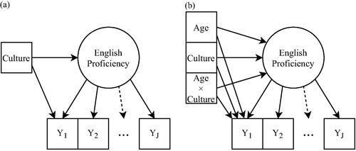
To evaluate MB, researchers often test for group differences (e.g., men vs. women) in item difficulty (intercept) and discrimination (factor loading) parameters, while controlling for differences in the latent variable distribution (Millsap, 2011). When one or more differences in the item parameters are statistically significant, this is often referred to as differential item functioning (DIF).¹ Figure 1a shows an example of this classical case, which is generally referred to as simple measurement bias. Common methods of evaluating simple MB include the use of modification indices/score tests with multiple-group confirmatory factor analysis (MG-CFA) models (Byrne et al., 1989), as well as likelihood ratio tests (Thissen et al., 1993) or Wald tests (Lord, 1977) with multiple-group item response theory (MG-IRT) models. In recent years, however, more flexible statistical methods have been developed to evaluate MB not only for a single categorical background variable at a time (e.g., culture), but also across multiple continuous and categorical variables simultaneously (e.g., culture, age, gender, socioeconomic status) as well as other complex relationships between background variables (e.g., age × culture). In particular, the moderated nonlinear factor analysis (MNLFA) model (Bauer & Hussong, 2009; Bauer, 2017) is a generalized latent variable approach (De Boeck & Wilson, 2004; Skrondal & Rabe-Hesketh, 2004) for evaluating multiple sources of MB on both item intercepts and factor loadings. Figure 1b shows an example of this modern case, which is referred to as complex measurement bias.

Figure 1. Two cases of measurement bias. (a) Simple measurement bias, where the group (e.g., cultural group) is the unit of analysis. (b) Complex measurement bias, where the individual (e.g., different ages across cultures) is the unit of analysis.

Until recently, the MNLFA approach faced a number of challenges that prevented researchers from taking advantage of its flexibility. The first major challenge was to accurately identify DIF among many potential background variable effects. A solution we proposed was to use a machine learning method commonly known as regularization, which demonstrated clear advantages of selecting DIF effects (i.e., fewer Type I errors) compared to traditional testing procedures (Bauer et al., 2020; Belzak & Bauer, 2020), particularly in larger sample sizes. The second major challenge for MNLFA was to efficiently estimate a large number of model parameters, as previous implementations became intractable with many item responses, background characteristics, and sample observations. We developed an alternative estimation approach, namely, a penalized expectation-maximization (EM) algorithm that more efficiently estimates a larger number of parameters in the MNLFA model (Belzak & Bauer, under review).

This paper addresses a third challenge—namely, a lack of didactic material and available software for using regularization to identify DIF in the MNLFA model. Thus, background information on measurement bias, the MNLFA model, and regularized DIF is provided in the following lines. The regDIF R package (Belzak, 2021) is then introduced, along with a tutorial using empirical examples and R code.

1. Background

1.1. Measurement/Item Bias

MB is formally defined as $f(\mathbf{y}|\theta )\ne f(\mathbf{y}|\theta ,\mathbf{x}),$ or the multivariate distribution of item responses, y, depends not only on the target latent variable, θ, but also on one or more exogenous variables, x (Meredith & Millsap, 1992; Millsap, 2011). All measurement models in this paper are assumed to be unidimensional—only one latent variable affects the item responses. Conversely, measurement invariance (MI) is defined as $f(\mathbf{y}|\theta )=f(\mathbf{y}|\theta ,\mathbf{x}),$ such that the item responses are independent of all exogenous variables after accounting for individual differences in the latent variable. Of course, there may be systematic differences in the latent variable as a function of the exogenous variables. This is referred to as impact and defined as $f(\theta )\ne f(\theta |\mathbf{x}).$ One goal of evaluating MB is to ensure that impact is valid.

Whereas MB and MI refer to the measure as a whole, DIF/item bias refers to a particular item. DIF is defined as $f({\mathbf{y}}_j|\theta )\ne f({\mathbf{y}}_j|\theta ,\mathbf{x}),$ with ${\mathbf{y}}_j$ referring to the responses for item j. MB implies that DIF is present for at least one item. However, DIF does not necessarily imply that MB occurs. In fact, the positive and negative effects of DIF could balance out across items, leading to MI. Differential test functioning (DTF; Chalmers et al., 2016) is one approach for evaluating this possibility.

Lastly, simple MB is distinguished from complex MB as the difference in the number of potential sources of bias. Akin to simple linear regression, simple MB is defined with respect to a single source of bias.² The evaluation of simple MB has been the predominant approach to DIF testing, which includes the MG-CFA and MG-IRT approaches. Conversely, complex MB is defined with respect to multiple sources of bias. This not only includes multiple conditional effects of background variables, but also interaction effects, mediation effects, and other causal relationships. MNLFA allows for the evaluation of both simple and complex MB. The latter is the focus below.

1.2. Model Specification

The MNLFA model (Bauer & Hussong, 2009) is specified using a formulation of the generalized linear model (GLM; McCullagh & Nelder, 2019). First, a linear predictor³ is defined: (1) $${\eta }_{ij}=({\nu }_{0j}+{\mathbf{x}}_i^T{\mathit{\nu }}_{1j})+({\lambda }_{0j}+{\mathbf{x}}_i^T{\mathbf{\lambda }}_{1j}){\theta }_i,$$(1) where ${\nu }_{0j}$ and ${\lambda }_{0j}$ represent the baseline intercept and slope, respectively, for item j when the background characteristics, ${\mathbf{x}}_i,$ for individual i equal 0. Conversely, ${\mathit{\nu }}_{1j}$ and ${\mathit{\lambda }}_{1j}$ represent individual differences in the intercept and slope relative to the baseline when one or more background characteristics are nonzero. In other words, ${\mathit{\nu }}_{1j}$ and ${\mathit{\lambda }}_{1j}$ are intercept and slope DIF effects (on item j) respectively. The latent score, θ_i, for individual i is also specified as a function of the background variables and assumed to be normally distributed: (2) $${\theta }_i\sim \mathcal{N}({\alpha }_i,{\psi }_i)$$(2) such that the latent mean, α_i, and latent variance, ψ_i, are defined: (3) $$\begin{array}{cc}{\alpha }_i\hfill & ={\alpha }_0+{\mathbf{x}}_i^T{\mathbf{\alpha }}_1,\hfill \\ {\psi }_i\hfill & ={\psi }_0\hspace{0.17em}\exp \hspace{0.17em}({\mathbf{x}}_i^T{\mathbf{\psi }}_1)\hfill \end{array}$$(3)

The baseline mean and variance parameters, α₀ and ψ₀ respectively, are fixed to 0 and 1 in the regDIF package to identify the model. Similar to (1), ${\mathit{\alpha }}_1$ and ${\mathit{\psi }}_1$ represent individual differences in the latent mean and variance as a function of the background variables, otherwise known as impact.

Secondly, a link function transforms the linear predictor into appropriate values of the item response, depending on how the response is distributed. For instance, if the item response, y_ij, is binary (e.g., yes/no, correct/incorrect), then $y_{ij}\sim \text{Bernoulli}({\mu }_{ij}),$ where μ_ij is the expected probability of individual i endorsing or correctly responding to item j. Then, a logistic function can link the expected probability to the linear predictor: (4) $${\mu }_{ij}=P(y_{ij}=1|{\eta }_{ij})=\frac{1}{1+\hspace{0.17em}\exp \hspace{0.17em}(-{\eta }_{ij})}.$$(4)

Other item responses may have different linear predictor(s) and link functions depending on the response distribution. For example, an ordinal item response (e.g., Likert-scaled) with C response categories has C − 1 linear predictors: (5) $$\begin{array}{cc}{\eta }_{0ij}\hfill & =({\nu }_{0j}+{\mathbf{x}}_i^T{\mathit{\nu }}_{1j})+({\lambda }_{0j}+{\mathbf{x}}_i^T{\mathbf{\lambda }}_{1j}){\theta }_i,\hfill \\ {\eta }_{1ij}\hfill & =({\nu }_{0j}+{\tau }_1+{\mathbf{x}}_i^T{\mathit{\nu }}_{1j})+({\lambda }_{0j}+{\mathbf{x}}_i^T{\mathbf{\lambda }}_{1j}){\theta }_i,\hfill \\ \hfill & ⋮\hfill \\ {\eta }_{(C-1)ij}\hfill & =({\nu }_{0j}+{\tau }_{(C-2)}+{\mathbf{x}}_i^T{\mathit{\nu }}_{1j})+({\lambda }_{0j}+{\mathbf{x}}_i^T{\mathbf{\lambda }}_{1j}){\theta }_i,\hfill \end{array}$$(5) which, in this parameterization, include C − 2 threshold parameters, τ₁, $\cdots ,{\tau }_{(C-2)},$ as well as a single baseline intercept, ${\nu }_{0j},$ present in all linear predictors.⁴ This assumes that DIF occurs in the intercept but not the threshold parameters, meaning that each linear predictor is shifted by an equal amount. In other words, there is only one set of DIF effects (intercept and slope) for each background characteristic.

The distribution of an ordinal item response is assumed $y_{ij}\sim \text{Categorical}({\mathit{\mu }}_{ij}),$ where ${\mathit{\mu }}_{ij}=\text{vec}({\mu }_{1ij},{\mu }_{2ij},\dots ,{\mu }_{\mathit{Cij}}).$ The link function can then be defined: (6) $${\mu }_{\mathit{cij}}=P(y_{ij}=c|{\eta }_{\mathit{cij}},{\eta }_{(c+1)ij})=\frac{1}{1+\hspace{0.17em}\exp \hspace{0.17em}(-{\eta }_{\mathit{cij}})}-\frac{1}{1+\hspace{0.17em}\exp \hspace{0.17em}(-{\eta }_{(c+1)ij})},$$(6) where c is the observed item response. Equation (6)(6) $${\mu }_{\mathit{cij}}=P(y_{ij}=c|{\eta }_{\mathit{cij}},{\eta }_{(c+1)ij})=\frac{1}{1+\hspace{0.17em}\exp \hspace{0.17em}(-{\eta }_{\mathit{cij}})}-\frac{1}{1+\hspace{0.17em}\exp \hspace{0.17em}(-{\eta }_{(c+1)ij})},$$(6) is Samejima’s (1969) graded response model.

Finally, for continuous item responses, the linear predictor is defined identically to (1), with the response distribution assumed $y_{ij}\sim \mathcal{N}({\mu }_{ij},{\sigma }_{ij}^2).$ This implies an identity link function, such that ${\mu }_{ij}={\eta }_{ij}.$ The response variance is ${\sigma }_{ij}^2={\sigma }_{0j}\hspace{0.17em}\exp \hspace{0.17em}({\mathbf{x}}_i^T{\sigma }_{1j}).$

Given that complex MB may be specified with the MNLFA model, the next step is to effectively distinguish real DIF effects from spurious DIF effects, the latter of which can appear due to sampling variability and model misspecification. Below, regularization is used to detect DIF among many potential sources of bias.

1.3. Regularized Differential Item Functioning

Regularization is a machine learning, data-driven method typically used to perform variable selection, and involves a penalty being appended to the model-fitting (likelihood/loss) function. In the MNLFA modeling framework, the penalty is applied to the DIF effects—${\mathit{\nu }}_{1j}$ and ${\mathit{\lambda }}_{1j}$—and works by shrinking all DIF effects towards zero as the value of a tuning parameter (shown in the next section) increases. Ultimately, a subset of DIF effects will shrink completely to zero as they fail to contribute to the model fit, thus removing these parameters and their corresponding background variables from the model. The goal of regularized differential item functioning (Reg-DIF) is to identify the optimal degree of penalization—that is, where DIF occurs in the measurement model and where it does not.

For DIF analysis, regularization is incorporated into the model-fitting function as such: (7) $$L_r({\varpi }_j|\theta ,\mathbf{x},{\mathbf{y}}_j)=L({\varpi }_j|\theta ,\mathbf{x},{\mathbf{y}}_j)-P({\mathit{\nu }}_{1j},{\mathbf{\lambda }}_{1j}|\tau ),$$(7) where $L_r({\varpi }_j|\theta ,\mathbf{x},{\mathbf{y}}_j)$ is the regularized model-fitting function for item j, which is maximized with respect to the item parameters, ${\varpi }_j=\text{vec}({\nu }_{0j},{\lambda }_{0j},{\mathit{\nu }}_{1j},{\mathit{\lambda }}_{1j}),$ conditional on the latent data, θ, and observed data, ${\mathbf{y}}_j$ and x; $L({\varpi }_j|\theta ,\mathbf{x},{\mathbf{y}}_j)$ is the model-fitting function without penalization; and $P({\mathit{\nu }}_{1j},{\mathit{\lambda }}_{1j}|\tau )$ is a general penalty function that depends on at least one tuning parameter, τ, although multiple tuning parameters are also possible.

The regularization procedure refers to the process of running multiple MNLFA models with varying levels of the tuning parameter or different magnitudes of penalization. Typically, a sequence of 100 values of τ is specified, with the largest value of τ corresponding to the model where all DIF effects are set to zero or removed from the model. There are a number of methods for selecting τ, including cross-validation (e.g., k-fold) and information criteria (e.g., Bayesian Information Criterion, BIC). We have found BIC to perform best in simulation studies (Bauer et al., 2020; Belzak & Bauer, 2020), particularly as the number of item responses, background variables, and sample observations grow large. Furthermore, there are a number of penalty functions that can be used for DIF analysis. These are illustrated below.

1.3.1. Least Absolute Shrinkage and Selection Operator

A notable penalty function is the LASSO (Tibshirani, 1996), or the least absolute shrinkage and selection operator. LASSO provides an efficient mechanism for selecting (background) variables by setting their corresponding parameter estimates (i.e., a subset of ${\mathit{\nu }}_{1j}$ and ${\mathit{\lambda }}_{1j}$) to zero during the regularization procedure. LASSO also aims to produce a sparse model, in which far fewer effects remain than what was initially considered. For DIF analysis, LASSO is written (8) $$P({\mathit{\nu }}_{1j},{\mathbf{\lambda }}_{1j};\tau )=\tau (|\left|{\mathit{\nu }}_{1j}\right|{|}_1+\left|\right|{\mathbf{\lambda }}_{1j}|{|}_1),$$(8) where τ denotes a tuning parameter that, when varied, augments the strength of penalization on the DIF effects, and $\left|\right|·|{|}_1$ is the L₁ norm, which takes the absolute value of each DIF effect and sums across all effects. Compared to classical approaches of DIF analysis (e.g., likelihood ratio testing, Thissen et al., 1993), LASSO has exhibited better recovery of DIF in a variety of conditions (Bauer et al., 2020; Belzak & Bauer, 2020). In particular, LASSO showed better control of Type I error (i.e., incorrectly identifying DIF) in larger sample sizes and scales with more pervasive DIF, while maintaining similar power to detect true DIF effects. LASSO is the default penalty method in regDIF.

1.3.2. Elastic Net

The elastic net penalty (Zou & Hastie, 2005) combines LASSO with the ridge penalty, the latter of which penalizes correlated predictors in tandem. The ridge penalty, by itself, is useful for dealing with model under-identification, particularly when highly correlated predictors are included together in a model. In contrast to LASSO, however, the ridge penalty (by itself) does not accomplish DIF selection. By combining LASSO with ridge, the elastic net thus achieves the advantages of both penalty methods by using a second tuning parameter, α, that controls the ratio of LASSO to ridge penalties. This is written (9) $$P({\mathit{\nu }}_{1j},{\mathbf{\lambda }}_{1j};\tau ,\alpha )=\tau [\alpha (\left|\right|{\mathit{\nu }}_{1j}|{|}_1+|\left|{\mathbf{\lambda }}_{1j}\right|{|}_1)+(1-\alpha )(\left|\right|{\mathit{\nu }}_{1j}|{|}_2+|\left|{\mathbf{\lambda }}_{1j}\right|{|}_2)],$$(9) where $\left|\right|·|{|}_2$ is the L₂ norm, which squares each DIF effect and sums across all effects. When α = 1, the elastic net penalty simplifies to the LASSO, and when α = 0, the elastic net simplifies to the ridge penalty. With two tuning parameters, τ and α, there is now a two-dimensional grid to search over for the optimal amount of penalization. To reduce the number of fitted models, researchers may first evaluate the grid in large increments of τ and α, and once a general region exhibits better fit, a second grid search can be done in smaller increments of the tuning parameters.

1.3.3. Minimax Concave Penalty

There is a bias-variance trade off when using LASSO and the elastic net (Friedman et al., 2010). Namely, these penalties introduce estimation bias as a means to reduce variance by a larger amount, thereby achieving lower mean squared error (i.e., ↓MSE = ↑bias${}^2+\downarrow$ variance). The Minimax Concave Penalty (MCP; Zhang, 2010) is an alternative to LASSO which aims to reduce bias while maintaining low variance. This is done using a second tuning parameter, denoted γ. For notational convenience, MCP is defined below with a single DIF parameter.⁵ This is written (10) $$P({\nu }_{1jk};\tau ,\gamma )=\{\begin{array}{cc}\tau \left|{\nu }_{1jk}\right|-\frac{{\nu }_{1jk}^2}{2\gamma },\hfill & \text{if}\left|{\nu }_{1jk}\right|\le \gamma \tau ;\hfill \\ \frac{1}{2}\gamma {\tau }^2,\hfill & \text{if}\left|{\nu }_{1jk}\right|>\gamma \tau ,\hfill \end{array}$$(10) where ${\nu }_{1jk}$ is the intercept DIF effect corresponding to the k-th background variable, and $\gamma >1$ is required. As $\gamma \to \infty ,$ MCP transforms into LASSO. Conversely, as $\gamma \to 1,$ MCP tapers the amount of bias induced by LASSO. In effect, MCP can be thought of as a scaling of LASSO. Despite the advantages of MCP, there is a trade off between larger values of γ (a more LASSO-like penalty) and smaller values of γ (more tapering of the LASSO penalty). Specifically, MCP runs into estimation issues where, in certain regions of optimizing the model-fitting function, the parameter estimates may no longer be unique.⁶ This leads to instability in parameter estimation. As such, researchers typically opt for a larger value of γ, such as γ = 3 (Breheny & Huang, 2011), and use different starting values to ensure the parameter estimates are unique. Both approaches are implemented in regDIF.

1.3.4. Group Penalties

Group penalty functions are used when sets of predictors are conceptually or quantitatively related and thus should be penalized (or kept) together in the model. This includes main effects with interactions and dummy-coded categorical variables. For DIF analysis, the intercept and slope DIF effects for each background variable is considered a group of predictors. Two group penalties implemented in regDIF are the group LASSO (Meier et al., 2008) and group MCP (Breheny & Huang, 2015). Although the math is beyond the scope of this paper (for details, see Belzak & Bauer, under review), the group MCP function is illustrated below using the regDIF package and empirical data.

In Table 1, the four types of penalty functions are compared.

Table 1. Comparison of penalty functions.

	LASSO^a	Elastic Net^b	MCP^c	Group
Description	Uses the L1 norm to penalize/select DIF effects; τ controls the magnitude of penalization	Uses a combination of the L1 and L2 norms to penalize/select DIF effects; τ controls the magnitude of penalization and α controls the degree of using a LASSO (L1) vs. Ridge (L2) penalty	Provides a continuum between the L0 “norm” and L1 norm to penalize/select DIF effects; τ controls the magnitude of penalization and γ controls the amount of estimation bias	Uses an extension of the LASSO/MCP functions
Benefits	Provides stable estimation of DIF effects; Only a single tuning parameter to toggle and select	Penalizes highly correlated predictors together; allows for more predictors than observations when α < 1	Provides less estimation bias; a default value of γ typically works well (e.g., γ = 3)	Selects groups of effects that are theoretically related (intercept and slope DIF effects of the same background variable)
Costs	Produces greater estimation bias in selected DIF effects; No options to reduce bias	Multiple tuning parameters to toggle and select	Can lead to unstable estimation of DIF effects with smaller γ (closer to L0 “norm”); Multiple tuning parameters to toggle and select	May require larger sample sizes to identify groups of intercept and slope DIF effects because slope DIF (interaction effect) is more difficult to identify

^aThe L₁ norm is the sum of absolute values of the DIF effects. ^bThe L₂ norm is the sum of squared values of the DIF effects. ^cThe L₀ “norm” is the number of non-zero DIF effects. “norm” is in quotation marks to indicate that it is not a proper norm, e.g., scaling the vector of DIF effects by a positive constant does not change the norm.

2. Software Implementation

regDIF (Belzak, 2021) is a package in the R statistical computing environment that provides a flexible implementation of Reg-DIF.⁷ The main function, regDIF(), allows for a variety of modeling possibilities, which include:

1. Multiple continuous and categorical background variables for DIF evaluation;

2. DIF evaluation without anchor items;

3. Binary, ordinal, and continuous item response functions;

4. LASSO, Elastic Net, Ridge, MCP, and group penalty functions; and

5. Observed proxy data in place of latent score estimation.

Each of these options are demonstrated below.

2.1. Getting Started with regDIF

First, regDIF can be installed and loaded into R with

install.packages(”regDIF”)

library(regDIF)

A simulated data set, ida, is available to users and generated to be consistent with Integrative Data Analysis (IDA; Curran & Hussong, 2009), where data are pooled across multiple independent studies. The first few rows of the data set can be viewed using

head(ida, 3)

Table

item1	item2	item3	item4	item5	item6	age	gender	study
0	0	0	0	0	0	-2	-1	-1
0	0	0	0	0	0	0	-1	-1
0	0	0	0	0	0	3	-1	-1

Specifically, 6 binary item responses (item1-item6) are outcomes of a normally-distributed latent variable, and DIF occurs between studies (study, effect-coded, on item 5) as well as within studies (age, mean-centered, on item 4; gender, effect-coded, on item 5). To accommodate the specification of regDIF(), the item response data should be separated from the predictor data (background variables):

item.data<- ida[, 1:6]

pred.data<- ida[, 7:9]

Second, it can be helpful to fit a model with all items designated as anchor items (i.e., DIF effects fixed to 0). This helps to examine the measurement model without accounting for DIF, taking note of the baseline item parameters and impact effect sizes. It also helps to gauge the speed of model estimation. Model estimation takes longer with more item responses, response options per item, background variables, and sample observations. The initial analysis is shown as

fit_initial<- regDIF(item.data,

                         pred.data,

                         tau = 0,

                         anchor = 1:ncol(item.data))

where the tuning parameter, tau, has been set to 0 (i.e., no penalization), and all items are designated as anchors. Note that regDIF() defaults to using the lasso penalty method. regDIF() also standardizes the predictors by default, a common recommendation in the regularization literature, such that all predictors are given equal weight during penalization. After estimation has finished, we can confirm that all DIF effects have been removed using the summary() method:

summary(fit_initial)

which shows, in order: (a) the function call, or the arguments given to the function; (b) the optimal model fit, corresponding to the value of tau; and (c) the non-zero DIF effects. As expected, no DIF effects remain in the model with all items as anchors. The model estimates can be viewed using the coef() method:

coef(fit_initial)

The output includes impact estimates, base(line) item estimates, and DIF estimates for each value of tau fit to the data. More specifically, the mean and variance impact estimates correspond to the values of ${\mathit{\alpha }}_1$ and ${\mathit{\psi }}_1$ in (3) respectively. The mean impact estimate of age, for example, can be interpreted as a .706 increase in the latent mean for every 1 SD increase in age, controlling for gender and study. The variance impact estimate of age can be interpreted as a .436 increase in the log of the latent variance for every 1 SD increase in age, controlling for gender and study. In addition, the base intercept (int) and slope (slp) item estimates correspond to the values of ${\nu }_{0j}$ and ${\lambda }_{0j}$ in (1) respectively, whereas the intercept and slope DIF effects correspond to the values of ${\mathit{\nu }}_{1j}$ and ${\mathit{\lambda }}_{1j}.$ Slope and intercept DIF effects are interpreted below.

Finally, the full regularization procedure can be fit to the data using

fit<- regDIF(item.data, pred.data)

which defaults to running 100 values of tau in varying increments (see num.tau argument in ?regDIF()). In particular, the procedure first identifies the minimum value of tau which removes all DIF from the model, then gradually reduces tau by increasingly smaller increments, and finally stops estimation once the model would become unidentified with too many DIF effects. Out of 100 models, the best-fitting model (according to BIC) is

summary(fit)

where four intercept DIF effects and two slope DIF effects were identified on items 4 and 5. Of the 6 effects identified, item5.int.age and item4.slp.study were misidentified (i.e., false positives), whereas the other four were correctly identified. Slope DIF for items 4 (age) and 5 (gender) were generated but unidentified (i.e., false negatives). The non-zero DIF effects can be interpreted as the following. Based on (1), for example, the intercept DIF effect of age on item 4 represents a .2153 increase in the log-odds of endorsing item 4 (binary response) for a 1 SD increase in age, controlling for gender and study. Conversely, the gender DIF effect of study on item 5 is an interaction between the latent variable (θ) and gender, such that the effect of θ on the log-odds of endorsing item 4 (i.e., the base slope) decreases by .1764 for a 1 SD increase in gender, controlling for age and study.

2.2. DIF Evaluation without Anchor Items

By starting the regularization procedure without DIF and allowing DIF effects to gradually enter the model with smaller degrees of penalization, anchor items are no longer required to evaluate DIF. This is a key advantage of Reg-DIF over classical testing procedures such as using likelihood ratio tests with MG-IRT (Thissen et al., 1993) or modification indices with MG-CFA (Byrne et al., 1989). In fact, Reg-DIF shows much better control of Type I error rates because it does not require anchor items (Bauer et al., 2020; Belzak & Bauer, 2020).

More specifically, as DIF effects enter the model and the value of tau decreases, regDIF() monitors the number of DIF effects that are present in the model. The model becomes unidentified when, for at least one background variable, there are as many intercept and/or slope DIF effects present in the model as there are item responses. With the ida data set, for instance, the model would be unidentified if intercept DIF for the age covariate was present for all 6 item responses. The regDIF() function automatically prevents this from happening by stopping the procedure. This results in NA values. What one hopes to see is that the best-fitting model (i.e., minimum value of BIC) occurs well before the model would have been unidentified. For the ida example above, this is viewed by plotting the values of BIC by the model number:

# Remove missing models.

bic_noNA<- fit$bic[!is.na(fit$bic)]

model_min_bic<- which.min(bic_noNA)

min_bic<- min(bic_noNA)

plot(bic_noNA,

     type=”l”,

     main=”Reg-DIF Path”, xlab=”Model Number”, ylab=”BIC”)

points(x = model_min_bic, y = min_bic,

        type=”b”, col=”red”, pch = 19)

Indeed, the minimum value of BIC (i.e., best-fitting model) occurs well before the model would have been unidentified.

2.3. Item Response Functions

In addition to binary item responses, regDIF() also supports ordinal and continuous item responses. Examples of both are shown using mental test scores of middle-school students across two different schools (Holzinger & Swineford, 1939). These data are available in the lavaan R package (Rosseel, 2012) and can be downloaded and organized with

# install.packages(lavaan)

item.data.hs<- lavaan::HolzingerSwineford1939[, 7:12]

pred.data.hs<- lavaan::HolzingerSwineford1939[, 2:6]

# Get total age, make grade a factor variable, and recode school

pred.data.hs$age<- pred.data.hs$ageyr + pred.data.hs$agemo / 12

pred.data.hs$grade<- as.factor(pred.data.hs$grade)

pred.data.hs$school<- ifelse(pred.data.hs$ school==”Pasteur”, 1, 0)

# Remove ageyr and agemo variables.

pred.data.hs$ageyr<- pred.data.hs$agemo<- NULL

Only the item responses corresponding to the “textual” and “visual” factors (i.e., first 6 items in Holzinger & Swineford, 1939) are examined together for DIF. These items showed higher inter-item correlation than the items corresponding to the “speed” factor (i.e., last 3 items in Holzinger & Swineford, 1939).

First, an MG-CFA is fit by treating the item responses as continuous and underlying a single latent variable (i.e. unidimensional), while using school as the grouping background variable. This is shown as

fit_hs_simple<- regDIF(item.data.hs, pred.data.hs$school,

                             item.type=”cfa”)

summary(fit_hs_simple)

where item.type =“cfa” specifies continuous responses. The model results show evidence of intercept DIF in items 1 and 3.

Second, to determine whether school is the main source of bias after controlling for other background variables, the model is ran using multiple predictors. This is shown

fit_hs_complex<- regDIF(item.data.hs, pred.data.hs, item.type=”cfa”)

summary(fit_hs_complex)

Indeed, school remains in the final model when controlling for sex, age, and grade. For continuous response data, summary() excludes residual DIF effects, which are never penalized and therefore always present during the regularization procedure.

Ordinal item responses can also be fit with regDIF(). One way to show this is by artificially cutting the continuous item responses into four equal quantiles:

item.data.hs.cat<-

 apply(item.data.hs, 2,

        function(x) {

          as.numeric(

            cut(x, breaks = summary(x)[-4], # Remove mean from break pts

                 include.lowest = T)

          )

       })

fit_hs_cat<- regDIF(item.data.hs.cat, pred.data.hs,

                         item.type=”graded”)

summary(fit_hs_cat)

Fewer DIF effects are selected for the final model, presumably because information has been lost by artificially categorizing the item responses. Note that there is only one intercept DIF effect for each background variable on item 3. This is a consequence of having a single baseline intercept for each background variable.

2.4. Penalty Methods

In addition to LASSO, there are a variety of other penalty methods implemented in regDIF(), including the elastic net and ridge penalties, MCP, and the group LASSO and group MCP functions. Examples of some are shown below using vocabulary data from the Duolingo English Test (DET; see technical manual, pp. 12–13, Cardwell et al., 2021).

The DET vocabulary data consisted of J = 18 words, some of which are real (e.g., “velvet”), and others which are fake but morphologically consistent with English (e.g., “vitalion”). N = 1586 test-takers were tasked with selecting the real English words. In effect, this constituted 18 binary item responses, corresponding to correct (1) and incorrect (0) responses. 6 of the 18 items were excluded from the analysis because more than 90% of the responses were correct, leaving 12 items in the final data set. Three background characteristics of test-takers were evaluated for DIF: gender, computer operating system, and age. A preview of these data are shown as

head(vocab_final, 3)

First, the elastic net penalty is demonstrated, where alpha in regDIF() controls the ratio of LASSO to ridge penalty functions. This is shown as

fit_net<- regDIF(vocab_final[, 1:12], vocab_final[, 13:15],

                     alpha=.5, control = list(maxit = 200))

summary(fit_net)

Intercept DIF in favor of females is identified for “velvet” and “disputning,” and in favor of males for “ruthless.” Age DIF is also identified in favor of older test-takers for “velvet,” “paradoxical,” and “materialism.” In the control argument, a maximum number of EM iterations is specified with maxit = 200. This prevents regDIF() from fitting models that would have been unidentified without the ridge penalty (embedded within the elastic net penalty).

Next, the MCP function is applied to the DET test data using pen.type = “mcp.” The default of gamma = 3 does not need to be explicitly specified as long as pen.type = “mcp.” This is shown as

fit_mcp<- regDIF(vocab_final[, 1:12], vocab_final[, 13:15],

                     pen.type=”mcp”)

summary(fit_mcp)

The same DIF effects identified with the elastic net model were also identified using MCP, in addition to intercept DIF in favor of older test-takers for “vitalion” and “ruthless,” and slope DIF in favor of younger test-takers for “materialism.” MCP produces larger magnitudes of DIF due to the tapering of tau via gamma. The plot() function shows how MCP removes the majority of DIF effects from the model while maintaining some DIF effects with less bias:

plot(fit_mcp)

That is, each line in the plot corresponds to an intercept or slope DIF effect. Viewing the plot from left to right, as the value of log(tau) decreases (i.e., less penalization), more DIF effects enter the model. The vertical dashed line corresponds to the value of log(tau) where BIC is at its minimum. Any effects that are non-zero at this point are considered to be DIF (dashed, colored lines), whereas the effects that remain zero are not considered to be DIF (gray lines). Finally, the jagged regions towards the right side of the figure show where the DIF estimates would be non-unique and unstable. Thus, it is important to visually examine the regularization path to ensure that the best-fitting model (i.e., model corresponding to the minimum value of BIC) does not occur in a region with heavy jagging.

Lastly, the group MCP function is demonstrated with

fit_mcpgroup<- regDIF(vocab_final[, 1:12], vocab_final[, 13:15],

                           pen.type=”grp.mcp”)

summary(fit_mcpgroup)

although no DIF effects were identified. Note that intercept and slope DIF will either be present or not in the model when using either the group MCP function or the group LASSO penalty (pen.type = “grp.lasso”).

2.5. Observed Data as Proxy to the Latent Variable

Due to the complexity of the model-fitting procedure, regDIF() can sometimes take a long time to finish running. For example, the simulated data example (6 binary items with 3 predictors) took approximately 9 minutes to fit all 100 values of tau on the regularization path. As the number of item responses, background characteristics, and sample observations increases, model estimation can become even slower. Therefore, a faster approach may be required for these types of applications. In particular, regDIF() allows for observed scores to be used as a proxy for latent scores. This simplifies the procedure to estimating a multivariate regression model, where the item responses are regressed on both the proxy data and background variables, and the proxy data are simultaneously regressed on the background variables. With proxy data, the time to fit a full regularization path decreases considerably; e.g., it took approximately 15 s to complete model-fitting. However, to the extent that the observed proxy has measurement error or is heavily affected by MB, this approach may lead to inaccurate DIF results. This is true for all observed methods of DIF identification, including logistic regression (Swaminathan & Rogers, 1990) and the Mantel-Haenszel method (Holland & Thayer, 1986).

An example using the DET vocabulary data is shown next, where the overall DET scores of test-takers serve as a proxy to the latent variable scores. DET scores are a linear combination of multiple types of reading, writing, listening, and speaking tasks (see Table 7 in Cardwell et al., 2021). Above, gender, age, and operating system were evaluated for DIF. Here, DIF is also examined as a function of 20 country-by-native-language categories. This includes Chinese test-takers whose native language is Mandarin Chinese, Indian test-takers whose native language is Hindi, and so on. The country-by-native-language categories were sum-coded, such that the effect of each category is defined as the difference between the average country-by-native-language effect. The LASSO penalty approach is specified with proxy data as

fit_proxy<- regDIF(vocab_final[, 1:12], vocab_final[, 13:35],

                        prox.data = det_score)

summary(fit_proxy)

Of the 23 background variables × 12 item responses × 2 intercept and slope effects, equaling 552 total DIF parameters, 16 DIF effects were ultimately identified with Reg-DIF. 11 of the 16 DIF effects are real English words, whereas the remaining effects are fake words. It is plausible that more DIF appears for real English words because the semantic content may tap into other aspects of a test-taker’s background (i.e., gender, culture, etc.). The fake words that show DIF may be close to real words (e.g., “disputning” is close to “disputing”), thus creating systematic distractions for some test-takers over others.

2.6. Additional Features

In addition to the key features of the regDIF package as illustrated above, there are other modeling possibilities available to the user. These include estimation of Expected a Posteriori (EAP) scores for the latent variable, comparing the effects of DIF on impact, and additional control over the model-fitting process. For instance, EAP scores and standard deviations can be recovered from the model-fit object using: fit$eap$scores and fit$eap$sd, where fit is the model-fit object. The effect of DIF on impact can be examined by comparing impact estimates obtained from the first model (all DIF has been set to zero) with impact estimates from the best-fitting model. This is achieved with: fit$impact[, which.min(fit$bic)] - fit$impact[, 1]. Finally, the control argument within the regDIF() function provides additional flexibility for specifying the Reg-DIF procedure. For example, different sets of predictors may be specified as effects of the latent variable (i.e., impact) using: control = list(impact.mean.data = pred.data2, impact.var.data = pred.data2), where pred.data2 is assumed to be a matrix of background variables that may or may not be a subset of the background variables that affect the item responses (i.e., DIF). Alternative optimization parameters may also be explicitly specified, such as smaller/larger convergence criteria, e.g., control = list(tol = 10^-7); the maximum number of EM iterations, e.g., control = list(maxit = 1,000); the number of quadrature points used to approximate the latent variable distribution, e.g., control = list(num.quad = 51); and the type of maximization technique, e.g., control = list(optim.method =“CD”), or coordinate descent optimization. Other options that are available can be viewed using? regDIF().

3. Concluding Remarks

The primary objectives of this paper were to (1) explain how a variety of regularization approaches can identify multiple sources of DIF within the MNLFA model, and to (2) demonstrate how these methods are implemented in the regDIF R package through empirical examples and code. This paper contributes to a growing literature of didactic material on using novel psychometric methods with open source software.

3.1. Limitations

It is important to point out that the regDIF package is in a constant state of development. The developmental version can be downloaded with: install.packages(devtools); devtools::install_github(“wbelzak/regDIF”). Some features that are currently in development are standard error estimation, multidimensional latent variable modeling, and count item response functions. Work is also underway to improve the speed of EM estimation. Slow model estimation is the main limitation of the regDIF R package. Namely, the regDIF() function can take tens of minutes and sometimes hours to fit larger data sets and models. Although better optimization of the source code can improve estimation speed, there may be an inherent limitation to how fast the EM algorithm can fit complex item response theory models. Other estimation approaches, such as a fine-tuned MCMC algorithm or limited-information estimators, may be better suited for fitting Reg-DIF models.

Another limitation of the Reg-DIF method is with respect to small sample sizes. Previous research has shown that Reg-DIF exhibits lower sensitivity (true positive rates) in small samples compared to other methods like likelihood ratio tests (Bauer et al., 2020). This implies that Reg-DIF is a large sample method. It also implies that where Reg-DIF performs best (in large samples) is also where model estimation takes the longest. Therefore, it is important that more research is done to improve the efficiency of Reg-DIF estimation. Future research should also evaluate the recovery of DIF while using proxy scores, especially since using proxy scores results in fast model estimation.

3.2. Recommendations

The goals of any DIF analysis should dictate which method of DIF detection to use. Based on the limitations noted above, the Reg-DIF method and the corresponding regDIF R package are most effective when large sample sizes are available and specificity (low false positives) is desirable. Conversely, if only small sample sizes are available and sensitivity is more desirable (high true positives), then the Reg-DIF method and regDIF package may not be the best approach. Alternatively, likelihood ratio tests are more powerful at identifying DIF in smaller sample sizes (Bauer et al., 2020).

If Reg-DIF is deemed an appropriate method for identifying DIF, evaluating the impact of DIF using the regDIF package is fairly straightforward. One approach is to first fit a model with all items designated as anchor items and collect the impact estimates, baseline item estimates, and EAP scores. Then, with the regDIF() function, identify the optimal amount of penalization and resultant DIF effects, and collect the impact estimates, baseline item estimates, and EAP scores from this DIF model. Any differences in the impact estimates, baseline item estimates, and EAP scores between the DIF model and anchor-item model can be interpreted as the effects of DIF. The advantage of this approach is that it avoids arbitrarily delineating meaningful effects from non-meaningful effects. Rather, the practitioner can examine the effect of DIF on different aspects of the model (e.g., item estimates, factor scores, etc.) to determine whether DIF is meaningful or not in the context of their data and research.

Taken together, the Reg-DIF method and the regDIF R package are novel psychometric tools for researchers who not only want to evaluate a single categorical background variable for measurement bias/invariance using regularization, but more importantly, who want to evaluate measurement bias across multiple sources of bias (i.e., referred to as complex measurement bias in the current article). Of course, there is more theoretical and computational work required to evaluate multiple sources of measurement bias in any given application. Nevertheless, the Reg-DIF method as implemented in the regDIF package is one step forward in the pursuit of better understanding the sources of measurement bias.

Notes

1 In theory, DIF does not depend on statistical significance, but rather on whether the conditional item response distribution varies as a function of a background characteristic, controlling for the latent variable.

2 Technically, simple MB has two predictors that affect the item responses: θ (latent variable) and x (exogenous variable). Simple MB refers to a single observed variable that is evaluated for bias.

3 A linear predictor is a linear combination of coefficients and covariates used to predict an outcome variable. Linear predictors are integral to the generalized linear modeling framework, where a variety of outcome types (e.g., continuous, binary, categorical, etc.) can all be specified using a linear predictor, a link function, and a distribution for the outcome.

4 By combining the baseline intercept with each threshold, we obtain C − 1 location parameters; the first location parameter is ${\nu }_{0j};$ the second is ${\nu }_{0j}-{\tau }_1;$ the third is ${\nu }_{0j}-{\tau }_2;$ and so on.

5 The multivariate extension applies the MCP penalty to each DIF effect simultaneously.

6 The likelihood function with MCP is not concave in some regions of the regularization path.

7 Reg-DIF refers to the method of using regularization to identify DIF across one or more sources of bias. regDIF refers to the R package that implements Reg-DIF. regDIF() refers to the main function in the regDIF R package.

References

- Bauer, D. J. (2017). A more general model for testing measurement invariance and differential item functioning. Psychological Methods, 22, 507–526. https://doi.org/10.1037/met0000077
- Bauer, D. J., Belzak, W. C. M., & Cole, V. T. (2020). Simplifying the assessment of measurement invariance over multiple background variables: Using regularized moderated nonlinear factor analysis to detect differential item functioning. Structural Equation Modeling, 27, 43–55.
- Bauer, D. J., & Hussong, A. M. (2009). Psychometric approaches for developing commensurate measures across independent studies: Traditional and new models. Psychological Methods, 14, 101–125.
- Belzak, W. C. M. (2021). regDIF: Regularized differential item functioning. Duolingo. R, version 1.1.0.
- Belzak, W. C. M., & Bauer, D. J. (2020). Improving the assessment of measurement invariance: Using regularization to select anchor items and identify differential item functioning. Psychological Methods, 25, 673–690. https://doi.org/10.1037/met0000253
- Belzak, W. C. M., & Bauer, D. J. (under review) Using regularization to identify measurement bias across multiple background characteristics: A penalized expectation-maximization algorithm.
- Breheny, P., & Huang, J. (2011). Coordinate descent algorithms for nonconvex penalized regression, with applications to biological feature selection. The Annals of Applied Statistics, 5, 232–253. https://doi.org/10.1214/10-AOAS388
- Breheny, P., & Huang, J. (2015). Group descent algorithms for nonconvex penalized linear and logistic regression models with grouped predictors. Statistics and Computing, 25, 173–187. https://doi.org/10.1007/s11222-013-9424-2
- Byrne, B. M., Shavelson, R. J., & Muthén, B. (1989). Testing for the equivalence of factor covariance and mean structures: The issue of partial measurement invariance. Psychological Bulletin, 105, 456.
- Cardwell, R., LaFlair, G. T., & Settles, B. (2021). Duolingo English Test: Technical manual. Duolingo Research Report, 1–37. https://duolingo-papers.s3.amazonaws.com/other/det-technical-manual-current.pdf
- Chalmers, R. P., Counsell, A., & Flora, D. B. (2016). It might not make a big dif: Improved differential test functioning statistics that account for sampling variability. Educational and Psychological Measurement, 76, 114–140.
- Curran, P. J., & Hussong, A. M. (2009). Integrative data analysis: The simultaneous analysis of multiple data sets. Psychological Methods, 14, 81–100. https://doi.org/10.1037/a0015914
- De Boeck, P., & Wilson, M. (2004). Explanatory item response models: A generalized linear and nonlinear approach. Spring-Verlag.
- Friedman, J., Hastie, T., & Tibshirani, R. (2010). Regularization paths for generalized linear models via coordinate descent. Journal of Statistical Software, 33, 1–22.
- Holland, P. W., & Thayer, D. T. (1986). Differential item functioning and the mantel-haenszel procedure. ETS Research Report Series, 1986, i–24. https://doi.org/10.1002/j.2330-8516.1986.tb00186.x
- Holzinger, K. J., & Swineford, F. (1939). A study in factor analysis: The stability of a bi-factor solution. Supplementary Educational Monographs.
- Lord, F. (1977). A study of item bias, using item characteristic curve theory. In Y. H. Poortinga (Ed.), Basic problems in cross-cultural psychology. Swets and Zeitlinger.
- McCullagh, P., & Nelder, J. A. (2019). Generalized linear models. Routledge.
- Meier, L., Van De Geer, S., & Bühlmann, P. (2008). The group lasso for logistic regression. Journal of the Royal Statistical Society: Series B (Statistical Methodology), 70, 53–71.
- Meredith, W., & Millsap, R. E. (1992). On the misuse of manifest variables in the detection of measurement bias. Psychometrika, 57, 289–311.
- Millsap, R. E. (2011). Statistical approaches to measurement invariance. Taylor & Francis Group.
- Rosseel, Y. (2012). Lavaan: An r package for structural equation modeling and more. Version 0.5–12 (beta). Journal of Statistical Software, 48, 1–36.
- Skrondal, A., & Rabe-Hesketh, S. (2004). Generalized latent variable modeling: Multilevel, longitudinal, and structural equation models. CRC Press.
- Swaminathan, H., & Rogers, H. J. (1990). Detecting differential item functioning using logistic regression procedures. Journal of Educational Measurement, 27, 361–370.
- Thissen, D., Steinberg, L., & Wainer, H. (1993). Detection of differential item functioning using the parameters of item response models. Lawrence Erlbaum Associates, Inc.
- Tibshirani, R. (1996). Regression shrinkage and selection via the lasso. Journal of the Royal Statistical Society: Series B (Methodological), 58, 267–288.
- Zhang, C.-H. (2010). Nearly unbiased variable selection under minimax concave penalty. The Annals of Statistics, 38, 894–942. https://doi.org/10.1214/09-AOS729
- Zou, H., & Hastie, T. (2005). Regularization and variable selection via the elastic net. Journal of the Royal Statistical Society: Series B (Statistical Methodology), 67, 301–320.