An Evaluation of Non-Iterative Estimators in Confirmatory Factor Analysis

Abstract

In confirmatory factor analysis (CFA), model parameters are usually estimated by iteratively minimizing the Maximum Likelihood (ML) fit function. In optimal circumstances, the ML estimator yields the desirable statistical properties of asymptotic unbiasedness, efficiency, normality, and consistency. In practice, however, real-life data tend to be far from optimal, making the algorithm prone to convergence failure, inadmissible solutions, and bias. In this study, we revisited some old, yet largely neglected non-iterative alternatives and compared their performance to more recently proposed procedures in an extensive simulation study. We conclude that closed-form expressions may serve as viable alternatives for ML, with the Multiple Group Method – the oldest method under consideration – showing favorable results across all settings.

Keywords:

• Confirmatory factor analysis
• maximum likelihood
• non-iterative estimation

1. Introduction

Confirmatory Factor Analysis (CFA) is a widely used multivariate analysis technique intended to account for relationships among a set of manifest variables. Since the early days of factor-analytic theory, items of psychological and educational test batteries are among the most frequently encountered variables of interest (see, for instance, Spearman’s seminal paper back in 1904 on the existence of a general intelligence factor). Applicability of factor-analytic models does, however, easily extend to other scientific disciplines such as criminology (e.g., Lussier et al., 2005), genomics (e.g., Yu et al., 2019) or medicine (e.g., Boyer et al., 2018).

Irrespective of the field of study, the aim of CFA models is to account for the $p(p+1)/2$ variances and covariances among p observed variables (i.e., indicators) by postulating the existence of two types of factors: (a) common factors that may affect more than one indicator, and (b) residual factors, which are indicator-specific. In a confirmatory setting, both the number of factors and the allocation of indicators to the factors draw upon subject matter theory and/or prior empirical results. Once the model is hypothesized, the unknown model parameters need to be estimated. For continuous (complete) data, this optimization problem is typically solved by minimizing the normal Maximum Likelihood (ML) discrepancy function. Some of the key characteristics of the resulting estimator are that, provided some assumptions, it is consistent, asymptotically unbiased, asymptotically efficient, and asymptotically normally distributed (Bollen, 1989; Silvey, 2017). Another noteworthy characteristic of the estimation procedure is that, except for very special cases, the minimum of the fit function cannot be obtained in closed form. Therefore, the search for ML estimates typically proceeds in an iterative manner.

Although the attractive statistical properties of the gold standard appear to avert the need for alternative estimators, ML yields its own challenges. When the validity of the underlying assumptions breaks down, for instance, the theoretical properties may no longer hold in practice. Especially in small to moderate samples, ML estimates are often systematically biased w.r.t. the true parameter value (Boomsma, 1985). Although it is guaranteed that this bias diminishes as the sample size moves to infinity, sample sizes in applied research are often (far) too small for asymptotic properties to hold. Other, more noticeable issues arise when the optimizer renders theoretically inadmissible solutions, or even no solution at all. The latter issue is known as non-convergence, which occurs when the iterative procedure fails to land on a stable solution.

Over the course of the previous century, a number of alternative estimation procedures have been proposed, such as the multiple group method (Guttman, 1944; 1952; Holzinger, 1944, Thurstone, 1945), FActor Analysis By INstrumental variables (FABIN, Hägglund, 1982), and the non-iterative CFA approach by Bentler (1982). Despite marked differences in underlying theory and implementation, all three methods have in common that they are non-iterative in nature. By transforming the complex optimization problem into a series of closed-form expressions, non-iterative methods obviate the need for complex iterative algorithms. Their simplicity leads to various attractive features, as they (a) cannot run into convergence issues, and (b) substantially reduce the computational burden. Because of these properties, their prime utility appears to be located at both ends of the data spectrum: in small samples (where they avoid frequently occurring convergence issues), as well as in big data with lots of indicators (where they substantially decrease computing time). Additionally, they can be implemented in such a way that they only allow for admissible solutions.

Notably, in spite of their intuitive appeal, studies looking into their performance are scarce, and present-day applied research using them presumably non-existent. Although at least one of them is currently being used under the hood (i.e., FABIN estimates operate as starting values for ML in several software programs), their apparent potential as self-contained estimation procedures remains largely untapped. Yet, from the handful of empirical evaluations that have been conducted (e.g., Hägglund, 1982, 1985; Stuive, 2007; Takane & Hwang, 2018), it appears that the fact that non-iterative methods have remained a somewhat neglected area in the field has little to do with their performance. From his Monte Carlo evaluation of the FABIN approaches, for instance, Hägglund (1985) concludes that in terms of parameter recovery, advantages for ML are usually small, and perhaps even negligible in practice. Similarly, Stuive (2007) reports promising results for the Multiple Group method, identifying the lack of implementation in common statistical software as its most important drawback.

As uncertainty prevails with respect to the relative merit of the aforementioned procedures, we set out to empirically evaluate their performance (convergence, admissibility of solutions, MSE) in an extensive Monte Carlo simulation study. Whereas it can be expected that ML will be undefeatable in ideal circumstances (e.g., large sample, normally distributed data, correctly specified model), non-iterative methods may well be sensible alternatives in settings where ML tends to perish and/or computational speed is desired. Aiming for a thorough comparison of both old and recent proposals, we revisit each of the aforementioned methods and compare their performance to ML (the default), ML using data-driven bounds (De Jonckere & Rosseel, 2022), and two other non-iterative alternatives: the more extensively researched Model-Implied Instrumental Variables via Two-Stage Least Squares (MIIV-2SLS, Bollen, 1996) and a recently proposed James–Stein type shrinkage estimator (Burghgraeve et al., 2021).

In what follows, we briefly describe each of the methods of interest (for detailed explanations, we kindly refer the reader to the original papers). Then, we report the design and results of our simulation study. We end with a summary of the results, along with a discussion of perceived opportunities and limitations.

2. The CFA Model

With p mean-centered indicators and k common factors, the factor-analytic model can be expressed by the following equation: (1) $$\mathit{y}=\mathbf{\Lambda }\mathit{\eta }+\mathit{ϵ}.$$(1)

Here, y is the $p\times 1$ random vector of indicators, $\mathbf{\Lambda }$ is the p × k matrix of factor loadings, $\mathit{\eta }$ is the $k\times 1$ vector of common factors, and $\mathit{ϵ}$ is the $p\times 1$ random vector of residuals. The k × k and p × p covariance matrices of $\mathit{\eta }$ and $\mathit{ϵ}$ are denoted $\mathbf{\Psi }$ and $\mathbf{\Theta },$ respectively. It is assumed that $\mathit{cov}(\mathit{\eta },\mathit{ϵ})=\mathit{0}.$ The model-implied variance-covariance matrix $\mathbf{\Sigma }$ is a function of all model parameters, gathered in a single vector of unknowns, $\mathit{\theta },$ and can be expressed as follows: (2) $$\mathbf{\Sigma }(\mathit{\theta })=\mathbf{\Lambda }\mathbf{\Psi }{\mathbf{\Lambda }}^T+\mathbf{\Theta }.$$(2)

3. Maximum Likelihood Estimation

The principle of ML is to find estimates for $\mathit{\theta }$ such that the likelihood of observing the sampled data is maximized. Under the assumption of multivariate normality, it can be shown that the values that maximize the likelihood of the data are the values that minimize the normal ML fit function: (3) $$F_{ML}(\mathit{\theta })=ln\left|\mathbf{\Sigma }\right|+tr(\mathit{S}{\mathbf{\Sigma }}^{-1})-ln\left|\mathit{S}\right|-p,$$(3) with $\mathbf{\Sigma }$ = $\mathbf{\Sigma }(\mathit{\theta })$ the model implied variance-covariance matrix, S the observed variance-covariance matrix, and p the number of indicators. Larger values of this function indicate a large discrepancy between the observed and model-implied covariance matrix, and hence, a poor model fit. In most cases, iterative methods are used to minimize the fit function (e.g., Gauss-Newton or quasi-Newton algorithms, see, for instance, Kochenderfer & Wheeler, 2019). This implies that some initial starting values are updated at every iteration until a predefined convergence criterion is reached. As recently proposed by De Jonckere and Rosseel (2022), this iterative process can be facilitated by imposing data-driven lower and upper bounds on the parameters.

4. Non-Iterative Estimation Procedures

4.1. Multiple Group Method

The first non-iterative method we will consider is the multiple group method as described in Guttman (1952, Section 5; not to be confused with Multiple Group CFA). Note, however, that an exhaustive overview of the development of this method would be incomplete without mentioning earlier work by Horst (1937), Holzinger (1944), Thurstone (1945), and Guttman (1944) – see Harman (1954, 1976).

The starting point for the analysis is the covariance matrix, S, where the diagonal elements are replaced by estimated communalities. In our implementations, we use the method from Spearman (1904) as described in Harman (1976, p. 115) to estimate these values per factor. For a given indicator y_i, the communality can be estimated as $$h_i^2=\frac{\sum _{j,k=1}^p\hspace{0.17em}{s}_{ij}{s}_{ik}}{\sum _{j,k=1}^p\hspace{0.17em}{s}_{jk}}$$ under the restrictions that $i\ne j,\hspace{0.17em}i\ne k,$ and $j<k.$ Note, however, that various alternative communality estimators exist; see, for instance, the numerous methods described in Harman (1976, Chapter 5) or the uniqueness estimator in Ihara and Kano (1986) and Cudeck (1991). Once the diagonal elements in S have been replaced by the estimated communalities, the resulting matrix is denoted by ${\mathit{S}}^{\mathit{*}}.$

In view of the hypothesized number of factors, we then divide the indicators in ${\mathit{S}}^{\mathit{*}}$ into k groups (hence the name “multiple group method”), and obtain two new matrices by summing specific elements. First, a k × p matrix ${\mathit{L}}_{\mathit{0}}$ is obtained by taking column-wise sums per group (i.e., for each indicator, we sum the elements within each group, the communality included). Then, a k × k matrix ${\mathit{P}}_{\mathit{0}}$ is obtained by taking row-wise sums in ${\mathit{L}}_{\mathit{0}},$ again for each group separately. Computationally, this can be achieved as follows: (4) $${\mathit{L}}_{\mathit{0}}={\mathit{X}}^{\mathit{T}}{\mathit{S}}^{\mathit{*}}$$(4) (5) $${\mathit{P}}_{\mathit{0}}={\mathit{X}}^{\mathit{T}}{\mathit{S}}^{\mathit{*}}\mathit{X},$$(5) where X is a p × k pattern matrix with binary elements reflecting the hypothesized grouping of indicators (i.e., a value of 1 whenever the indicator is assumed to reflect the underlying factor and zero elsewhere). After multiplication by the appropriate scaling factors, we obtain the factor structure matrix, L, and the factor correlation matrix, P: (6) $$\mathit{L}={\mathit{L}}_{\mathit{0}}{\mathit{D}}^{\mathit{-1/2}}$$(6) (7) $$\mathit{P}={\mathit{D}}^{\mathit{-1/2}}{\mathit{P}}_{\mathit{0}}{\mathit{D}}^{\mathit{-1/2}},$$(7) where D denotes a diagonal matrix with the same diagonal as ${\mathit{P}}_{\mathit{0}}.$ From L, we arrive at the (unconstrained) factor loadings by multiplying by the inverse of P: (8) $${\mathbf{\Lambda }}^{*}=\mathit{L}{\mathit{P}}^{\mathit{-1}}$$(8)

In order to enforce simple structure on the loadings, constrained methods can be used to solve (8). In our implementations, we translated the estimator in a constrained quadratic program. Final estimates of $\mathbf{\Lambda }$ and $\mathbf{\Psi }$ are obtained by (9) $$\mathbf{\Psi }=\mathit{MPM}$$(9) (10) $$\mathbf{\Lambda }={\mathbf{\Lambda }}^{*}{\mathit{M}}^{\mathit{-1}},$$(10) where M is a k × k diagonal matrix with the loadings of the scaling indicators as its diagonal elements. Post-multiplying ${\mathbf{\Lambda }}^{*}$ with the inverse of this matrix ensures that the scaling indicators now have unit loading on their respective factors.

4.2. Hägglund’s Instrumental Variable Approach

Almost two decades after Madansky (1964) coined the idea of using instrumental variables in estimating factor analytic models, Hägglund (1982) introduced three alternative Factor Analysis By INstrumental variables (FABIN) procedures: FABIN1, FABIN2, and FABIN3. The central idea of these procedures is that the model in Equation (1)(1) $$\mathit{y}=\mathbf{\Lambda }\mathit{\eta }+\mathit{ϵ}.$$(1) can be rewritten as a system of linear equations with errors in variables. Assuming that $p\ge 3k,$ we partition the indicators into three sets with k indicators in the first, q indicators in the second, and r indicators in the third: (11) $$\underset{k\times 1}{\underbrace{{\mathit{y}}_{\mathit{1}}}}=\underset{k\times k}{\underbrace{{\mathbf{\Lambda }}_{\mathbf{1}}}}\underset{k\times 1}{\underbrace{\mathit{\eta }}}+\underset{k\times 1}{\underbrace{{\mathit{ϵ}}_{\mathit{1}}}}$$(11) (12) $$\underset{q\times 1}{\underbrace{{\mathit{y}}_{\mathit{2}}}}=\underset{q\times k}{\underbrace{{\mathbf{\Lambda }}_{\mathbf{2}}}}\underset{k\times 1}{\underbrace{\mathit{\eta }}}+\underset{q\times 1}{\underbrace{{\mathit{ϵ}}_{\mathit{2}}}}$$(12) (13) $$\underset{r\times 1}{\underbrace{{\mathit{y}}_{\mathit{3}}}}=\underset{r\times k}{\underbrace{{\mathbf{\Lambda }}_{\mathbf{3}}}}\underset{k\times 1}{\underbrace{\mathit{\eta }}}+\underset{r\times 1}{\underbrace{{\mathit{ϵ}}_{\mathit{3}}}}.$$(13)

With the variables in ${\mathit{y}}_{\mathit{1}}$ serving as scaling indicators, we set ${\mathbf{\Lambda }}_{\mathbf{1}}$ to identity. Solving (11) for $\mathit{\eta }$ then gives us $\mathit{\eta }={\mathit{y}}_{\mathit{1}}-{\mathit{ϵ}}_{\mathit{1}}.$ This expression can now be substituted into (12): (14) $$\begin{array}{c}{\mathit{y}}_{\mathit{2}}={\mathbf{\Lambda }}_{\mathbf{2}}({\mathit{y}}_{\mathit{1}}-{\mathit{ϵ}}_{\mathit{1}})+{\mathit{ϵ}}_{\mathit{2}}\\ \hspace{1em}\hspace{1em}={\mathbf{\Lambda }}_{\mathbf{2}}{\mathit{y}}_{\mathit{1}}+{\mathit{ϵ}}_{\mathit{2}}-{\mathbf{\Lambda }}_{\mathbf{2}}{\mathit{ϵ}}_{\mathit{1}}.\end{array}$$(14)

The estimation problem now resembles conventional linear regression with the variables in ${\mathit{y}}_{\mathit{1}}$ as explanatory variables and $\widetilde{\mathit{ϵ}}={\mathit{ϵ}}_{\mathit{2}}-{\mathbf{\Lambda }}_{\mathbf{2}}{\mathit{ϵ}}_{\mathit{1}}$ representing a composite error term. Note, however, that since ${\mathit{y}}_{\mathit{1}}$ is correlated with ${\mathit{ϵ}}_{\mathit{1}},$ the explanatory variables in this equation are no longer uncorrelated with the error term $\widetilde{\mathit{ϵ}}.$ As this violates the zero conditional mean assumption, Least Squares cannot be used to estimate the remaining unknowns. It is here that instrumental variables come into play: as the variables in ${\mathit{y}}_{\mathit{3}}$ are correlated with the endogenous variables but uncorrelated with the error term, they can serve as instruments in determining ${\mathbf{\Lambda }}_{\mathbf{2}}.$ Because algebraic manipulation of (14) gives us ${\mathit{ϵ}}_{\mathit{2}}-{\mathbf{\Lambda }}_{\mathbf{2}}{\mathit{ϵ}}_{\mathit{1}}={\mathit{y}}_{\mathit{2}}-{\mathbf{\Lambda }}_{\mathbf{2}}{\mathit{y}}_{\mathit{1}},$ it must hold that (15) $$E[{\mathit{y}}_{\mathit{3}}({\mathit{y}}_{\mathit{2}}-{\mathbf{\Lambda }}_{\mathbf{2}}{\mathit{y}}_{\mathit{1}})\prime ]=\mathit{0}.$$(15)

With ${\mathbf{\Sigma }}_{ij}=E[{\mathit{y}}_{\mathit{i}}\mathit{y}{\prime }_{\mathit{j}}],$ this leads to ${\mathbf{\Sigma }}_{\mathbf{32}}={\mathbf{\Sigma }}_{\mathbf{31}}{\mathbf{\Lambda }}_{\mathbf{2}},$ or equivalently, ${\mathbf{\Sigma }}_{\mathbf{23}}={\mathbf{\Lambda }}_{\mathbf{2}}{\mathbf{\Sigma }}_{\mathbf{13}}.$ After postmultiplication by ${\mathbf{\Sigma }}_{\mathbf{31}}$ we get ${\mathbf{\Sigma }}_{\mathbf{23}}{\mathbf{\Sigma }}_{\mathbf{31}}={\mathbf{\Lambda }}_{\mathbf{2}}{\mathbf{\Sigma }}_{\mathbf{13}}{\mathbf{\Sigma }}_{\mathbf{31}}.$ Replacing the covariance submatrices by their sample counterparts, we obtain the FABIN1 estimator: (16) $${\stackrel{\mathbf{⁁}}{\mathbf{\Lambda }}}_{\mathbf{2}}=\hspace{0.17em}{\mathit{S}}_{\mathbf{23}}{\mathit{S}}_{\mathbf{31}}{({\mathit{S}}_{\mathbf{13}}{\mathit{S}}_{\mathbf{31}})}^{-1}.$$(16)

The usual zero restrictions in a confirmatory case can be induced by restricting the dimensions of the matrices involved (i.e., omitting indicators in ${\mathbf{y}}_{\mathbf{1}}$ that serve as scaling indicators for factors on which the indicator in ${\mathbf{y}}_{\mathbf{2}}$ does not load; see Hägglund, 1985). Estimates for ${\mathbf{\Lambda }}_{\mathbf{3}}$ can be obtained in a similar fashion, using the indicators in ${\mathit{y}}_{\mathbf{2}}$ as instruments.

Although FABIN1 yields consistent estimates, the choice of variables in each set may present substantial difficulties. A modified estimator, FABIN2, resolves this issue by restricting q to equal 1 (i.e., allowing only one variable in the second set) and using all $p-k-1$ variables in ${\mathit{y}}_{\mathbf{3}}$ as instruments. The resulting expression for FABIN2 is highly similar to (16) with the submatrix ${\mathit{S}}_{\mathbf{23}}$ now being a row vector of covariances: (17) $${\stackrel{\mathbf{⁁}}{\mathbf{\Lambda }}}_{\mathbf{2}}=\hspace{0.17em}{\mathit{s}}_{\mathbf{23}}{\mathit{S}}_{\mathbf{31}}{({\mathit{S}}_{\mathbf{13}}{\mathit{S}}_{\mathbf{31}})}^{-1}.$$(17)

By alternating the variables in ${\mathit{y}}_{\mathit{2}}$ (each time using the remaining $p-k-1$ variables in ${\mathit{y}}_{\mathit{3}}$), factor loading estimates are obtained in a successive manner. With this modified estimator, the only subjective decision left is the choice of reference variables in ${\mathit{y}}_{\mathbf{1}}.$

A final modification of the estimation procedure leads to a Weighted Least Squares (LS) solution, called FABIN3: (18) $${\stackrel{\mathbf{⁁}}{\mathbf{\Lambda }}}_{\mathbf{2}}=\hspace{0.17em}{\mathit{s}}_{\mathbf{23}}{\mathit{S}}_{\mathbf{33}}^{-\mathit{1}}{\mathit{S}}_{\mathbf{31}}{({\mathit{S}}_{\mathbf{13}}{\mathit{S}}_{\mathbf{33}}^{-\mathbf{1}}{\mathit{S}}_{\mathbf{31}})}^{-1}.$$(18)

FABIN3 is called a Two-Stage Least Squares (2SLS) estimator since it may be obtained from (14) by regressing the endogenous variables on the instruments in a first stage, and then regressing ${\mathit{y}}_{\mathit{2}}$ on the predictions ${\widehat{\mathit{y}}}_{\mathit{1}}$ instead of ${\mathit{y}}_{\mathit{1}}$ in a second stage. Given the estimates for the loadings, estimates for $\mathbf{\Psi }$ and $\mathbf{\Theta }$ can be found by minimizing $Q=tr({\mathit{A}}^2)$ with $\mathit{A}=\mathit{S}-\stackrel{\mathbf{⁁}}{\mathbf{\Lambda }}\mathbf{\Psi }{\stackrel{\mathbf{⁁}}{\mathbf{\Lambda }}}^T-\mathbf{\Theta }$ according to the Least Squares principle (see Hägglund, 1982; Section 4 for derivations). Alternatively, as advocated by Jennrich (1987), a Weighted LS version (Browne, 1974) can be used using ${\mathit{S}}^{\mathit{-1}}$ as a weight matrix. Although the FABIN estimators assume that $\mathbf{\Theta }$ is diagonal, they can be adapted to allow for correlated errors by a more stringent selection of instrumental variables in ${\mathit{y}}_{\mathit{3}}$ (Bollen, 1989, 1996; see infra).

4.3. Bentler’s Non-Iterative Estimation Procedure

Shortly after Hägglund introduced FABIN, Bentler (1982) proposed yet another non-iterative procedure that draws upon the partitioning of the covariance matrix. We again divide the indicators into different sets: a first set (${\mathit{y}}_{\mathit{1}}$) with k scaling indicators, and a second set (${\mathit{y}}_{\mathit{2}}$) with the remaining p – k indicators. With the variables in ${\mathit{y}}_{\mathit{1}}$ having unit loadings on their respective factors, we obtain the following expressions: (19) $${\mathit{y}}_{\mathit{1}}={\mathbf{\Lambda }}_{\mathbf{1}}\mathit{\eta }+{\mathit{ϵ}}_{\mathit{1}}$$(19) (20) $${\mathit{y}}_{\mathit{2}}={\mathbf{\Lambda }}_{\mathbf{2}}\mathit{\eta }+{\mathit{ϵ}}_{\mathit{2}},$$(20) where ${\mathbf{\Lambda }}_{\mathbf{1}}$ equals the identity matrix. These expressions lead to the following decomposition of covariances: (21) $${\mathbf{\Sigma }}_{\mathbf{11}}=\mathbf{\Psi }+{\mathbf{\Theta }}_{\mathbf{1}}$$(21) (22) $${\mathbf{\Sigma }}_{\mathbf{21}}={\mathbf{\Lambda }}_{\mathbf{2}}\mathbf{\Psi }$$(22) (23) $${\mathbf{\Sigma }}_{\mathbf{22}}={\mathbf{\Lambda }}_{\mathbf{2}}\mathbf{\Psi }{\mathbf{\Lambda }}_{\mathbf{2}}^{\prime }+{\mathbf{\Theta }}_{\mathbf{2}}.$$(23)

Given (22), we can rewrite (23) as follows: (24) $${\mathbf{\Sigma }}_{\mathbf{22}}={\mathbf{\Sigma }}_{\mathbf{21}}{\mathbf{\Psi }}^{-1}{\mathbf{\Sigma }}_{\mathbf{21}}^{\prime }+{\mathbf{\Theta }}_{\mathbf{2}}.$$(24)

The key of the method is that by replacing ${\mathbf{\Sigma }}_{\mathbf{21}}$ by its sample counterpart ${\mathit{S}}_{\mathit{21}},$ the estimation problem in (24) is reduced to a linear function of the remaining parameters. As a result, we can now use Unweighted or Weighted LS to obtain estimates for ${\mathbf{\Psi }}^{-\mathbf{1}}$ and ${\mathbf{\Theta }}_{\mathbf{2}}.$ Once these are found, ${\mathbf{\Theta }}_{\mathbf{1}}$ and ${\mathbf{\Lambda }}_{\mathbf{2}}$ can be estimated as follows: (25) $${\stackrel{\mathbf{⁁}}{\mathbf{\Theta }}}_{\mathbf{1}}=\hspace{0.17em}\hspace{0.17em}{\mathit{S}}_{\mathit{11}}-\stackrel{\mathbf{⁁}}{\mathbf{\Psi }}$$(25) (26) $${\stackrel{\mathbf{⁁}}{\mathbf{\Lambda }}}_{\mathbf{2}}=\hspace{0.17em}\hspace{0.17em}{\mathit{S}}_{\mathit{21}}{\stackrel{\mathbf{⁁}}{\mathbf{\Psi }}}^{-\mathbf{1}}$$(26)

In a confirmatory setting, constrained methods can be used to set certain elements of ${\stackrel{\mathbf{⁁}}{\mathbf{\Lambda }}}_{\mathbf{2}}$ to zero (Bentler, 1982; p. 419). In our implementations, we translated the LS estimator in (26) into a constrained quadratic program to satisfy the hypothesized constraints on the loadings.

4.4. Bollen’s MIIV-2SLS

Whereas the previously discussed non-iterative approaches were all concerned with the estimation of CFA models, the Model-Implied Instrumental Variables via Two-Stage Least Square (MIIV-2SLS) approach proposed by Bollen (1996) is more generally applicable to full Structural Equation Models (SEMs) that do not only specify the relationships between indicators and their underlying factors, but also relationships between these factors themselves. Contrary to the other approaches, MIIV-2SLS is also more conveniently accessible to applied users as a dedicated software package is available in R (MIIVsem; Fisher et al., 2021). Merely focusing on the factor loadings in the measurement model, the estimation procedure is closely related to Hägglund’s FABIN3 estimator in (18). Differences between the methods present themselves in terms of the indicators that are being used as instruments. In contrast to FABIN, MIIV-2SLS allows the off-diagonal elements of $\mathbf{\Theta }$ to be non-zero. This implies that some of the previously eligible instruments may no longer be uncorrelated with the composite error term (Bollen, 1989; p. 415). As such, the set of instruments needs to be pruned to accommodate the correlated error matrix. In addition, whereas Hägglund searches for instruments in the $p-k-1$ indicators (thereby excluding all k scaling indicators to serve as instruments in other equations), MIIVsem does allow scaling indicators to be used as instruments when appropriate. Using a different set of instruments inevitably leads to (small) differences in point estimates, especially for smaller models where the number of possible instruments is already small.

Another difference between the methods concerns the steps that are being taken once $\mathbf{\Lambda }$ is estimated. More specifically, MIIVsem does not provide estimates for $\mathbf{\Psi }$ and $\mathbf{\Theta }$ unless it is explicitly asked to do so via the “var.cov” argument. If set to TRUE, point estimates for the variance parameters are obtained by optimizing the ML fit function with the estimated loadings considered fixed (cf. Bollen, 1996; p. 117).

4.5. James-Stein Type Shrinkage Estimator

Recently, Burghgraeve et al. (2021) proposed an alternative procedure to estimate SEMs non-iteratively. Similar to FABIN and MIIV-2SLS, the spirit of the method is to replace the latent variable by an estimable quantity that is uncorrelated with the error term. However, instead of replacing the latent variable by the scaling indicator minus its error and using instruments to resolve the resulting endogeneity issue, the authors propose to replace the latent variable by its conditional expectation given the scaling indicator. With y_ij being the j^th indicator of the i^th latent variable, and $y_{i1}$ denoting the scaling indicator, the model can be rewritten as (27) $$y_{ij}={\lambda }_{ij}\mathbb{E}({\eta }_i|y_{i1})+{\overline{ϵ}}_{ij},$$(27) where ${\overline{ϵ}}_{ij}={\lambda }_{ij}({\eta }_i-\mathbb{E}({\eta }_i|y_{i1}))+{ϵ}_{ij}.$ The conditional expectation can be expressed as (28) $$\mathbb{E}({\eta }_i|y_{i1})=R_i{y}_{i1}+(1-R_i)\mathbb{E}({\eta }_i),$$(28) where R_i denotes the reliability of $y_{i1}.$ It can be estimated by plugging in the sample mean of $y_{i1}$ as an estimator for $\mathbb{E}({\eta }_i),$ and estimating $(1-R_i)$ as (29) $$\widehat{1-R_i}\frac{(n-3)\hspace{0.17em}\widehat{\mathit{var}\left({ϵ}_{i1}\right)}}{(n-1)\hspace{0.17em}\widehat{\mathit{var}(y_{i1})}},$$(29) where $\widehat{\mathit{var}(y_{i1})}$ and $\widehat{\mathit{var}({ϵ}_{i1})}$ denote the unbiased sample variance and the residual variance of the scaling indicator. The authors propose that the latter quantity can be estimated via the method described in Harman (1976; Section 7.2) based on Spearman (1904, 1927). Note that Equation (28)(28) $$\mathbb{E}({\eta }_i|y_{i1})=R_i{y}_{i1}+(1-R_i)\mathbb{E}({\eta }_i),$$(28) is a shrinkage estimator as it shrinks $\widehat{\mathbb{E}({\eta }_i|y_{i1})}$ from the observed values in $y_{i1}$ towards their mean as the reliability of the scaling indicator decreases. Once the conditional expectation is estimated, the remaining parameters in (27) can be estimated using conventional LS.

Conditioning on the scaling indicator, the aforementioned estimator is referred to as the scaling James-Stein. An alternative estimator, referred to as aggregated James-Stein, makes better use of all available data as it conditions on a data-driven aggregation of the indicators, $y_i^{\mathit{agg}}={\mathit{w}}_{\mathit{i}}^{\prime }{\mathit{y}}_{\mathit{i}},$ where ${\mathit{y}}_{\mathit{i}}$ comprises all indicators for that factor except for the one whose loading we wish to estimate, and the weight vector ${\mathit{w}}_{\mathit{i}}$ is chosen to maximize the estimated reliability of $y_i^{\mathit{agg}}.$

4.6. Potential Challenges for Non-Iterative Methods

Thus far, we have implicitly assumed that a complete data set is at our disposal. Yet, in practice, researchers often have to deal with missing entries. Different solutions exist when this is the case (see, for instance, Enders, 2001). The most straightforward approach is to omit all incomplete cases (i.e., listwise deletion), and perform all further computations on the covariance matrix for the remaining cases. Although applicable for all estimation procedures, discarding part of the data results in a loss of precision, as well as biased estimates when the missing-data mechanism is not MCAR (Missing Completely At Random; see Little & Rubin, 2019 for a classification of missingness mechanisms). For ML, a well-known alternative is known as Full Information ML (FIML), which permits to use also partially available data by computing casewise likelihoods, each time using only those variables that are observed for a particular case. This approach is more appealing from a statistical perspective, as it is characterized by higher power and unbiasedness under both MAR (Missing At Random) and MCAR missingness. Optimizing an accumulated likelihood function, it is evident that FIML does not pertain to the aforementioned closed-form expressions. A potential concern might therefore be how non-iterative procedures are able to deal with missing data. In this regard, we would like to remind the reader that there are also other ways to tackle missing data. A first alternative is to adopt a two-step procedure where we first estimate the covariance matrix via an Expectation-Maximization (EM) algorithm (step 1), which can then be used as input for the usual complete-data procedures (step 2). A second alternative, known as multiple imputation (Rubin, 1987), creates different imputed versions of the data. Each of these versions will yield different parameter estimates, which can then be averaged to produce a single set of (pooled) results. Similar to FIML, both the two-step approach and multiple imputation have the advantage of also being unbiased under MAR, although it is important to note that standard errors and test statistics need to be corrected to account for the additional uncertainty that arises from estimating the covariance matrix (Newman, 2014; Savalei & Bentler, 2009; Savalei & Falk, 2014) or imputing the missing entries (Rubin, 1987).

A second conceivable concern is how equality constraints can be imposed on certain parameters in the model. When computing Cronbach’s alpha (Cronbach, 1951), for example, it is assumed that all indicators have the same relationship with the underlying factor (i.e., tau equivalence). Put differently, it is assumed that the factor loadings are equal. In order to establish a tau equivalent measurement model, loadings would need to be estimated (like any other free parameters) but should be constrained such that they can only take on one common value. Although the details of possible implementations are beyond the scope of this article, we would like to point out that even though equality constraints evoke some additional complications, they do not necessarily impede the use of the non-iterative estimators; see, for instance, Bentler (1982), Nestler (2014), and Toyoda (1997).

A final apparent drawback of stepping outside the Maximum Likelihood framework is that one can no longer use the usual ML standard errors and goodness-of-fit measures. Yet, this does not imply that the use of non-iterative procedures is limited to point estimation. For the instrumental variable approaches (Bollen, 1989; Hägglund, 1982), for instance, analytic expressions are available to estimate the respective standard errors. Alternatively, an empirical estimate of the variability of the estimator can be obtained by use of resampling procedures. To evaluate whether the model actually fits the observed data, various alternative fit measures can be considered. Within the MIIV-2SLS framework, local fit measures (Kirby & Bollen, 2009; Sargan, 1958) already belong to the standard output of this analysis. For global fit measures (e.g., the chi-square test statistic, CFI, RMSEA,…), a possible avenue is to compute the model-implied summary statistics from the individual estimates, and use these to obtain “pseudo” versions of the traditional indices (see, for instance, Devlieger et al., 2019, for an extensive evaluation in the context of factor score regression).

4.7. Numerical Example

To illustrate how estimates from different estimation procedures can either coincide or diverge depending on the circumstances, we gathered estimates for two randomly simulated datasets with either a very large or a very small sample size ($n=100000,n=10$), in otherwise good conditions (i.e., no misspecification, normal data). Population values of the model are found in the Appendix A; R code for these and all further analyses can be found in our OSF repository via the following link: https://osf.io/ufqsc/. Part of the estimated values are shown in Table 1. In the large sample setting, all estimates are close to the population values, and hence also close to one another. This does not hold for the small sample setting, where large discrepancies between methods emerge, and some estimators approach the data generating values better than others. Given that elaborate evaluations of most of the non-iterative methods are scarce, it is yet to be determined how the relative ranking of methods in this example would generalize across data sets, and by extension, across circumstances (e.g., in the presence of structural and/or distributional misspecifications).

Table 1. Numerical example with simulated data showing how different estimation procedures can yield very similar results in optimal conditions (here: very large sample size), but also very different results in suboptimal conditions (here: very small sample size).

	n = 100,000				n = 10
	${\lambda }_{6,2}$	${\theta }_{6,6}$	${\psi }_{2,2}$	${\psi }_{2,1}$	${\lambda }_{6,2}$	${\theta }_{6,6}$	${\psi }_{2,2}$	${\psi }_{2,1}$
	0.8	1.0	1.0	0.5	0.8	1.0	1.0	0.5
ML	0.796	0.998	1.003	0.497	4.259	−3.123	0.345	−0.032
MLB	0.796	0.998	1.003	0.497	1.624	0.000	1.188	0.129
Multiple group	0.795	0.997	1.011	0.499	1.225	0.393	1.837	0.285
FABIN 2 – ULS	0.798	0.998	1.002	0.496	1.109	0.882	2.069	0.204
FABIN 3 – ULS	0.796	0.998	1.006	0.498	0.801	1.407	2.414	0.343
FABIN 2 – WLS	0.798	0.998	1.002	0.496	1.109	0.005	1.076	−0.224
FABIN 2 – WLS	0.796	0.998	1.006	0.498	0.801	0.011	0.553	0.081
Bentler – ULS	0.797	0.997	1.006	0.498	1.046	0.000	1.845	0.025
Bentler – WLS	0.796	0.996	1.006	0.498	0.799	0.000	2.414	−0.096
MIIV-2SLS	0.795	0.999	1.004	0.498	0.827	0.434	3.210	0.410
JS scaling	0.794	0.997	1.012	0.499	1.203	0.393	1.927	0.294
JS aggregated	0.794	0.997	1.012	0.499	1.185	0.393	1.959	0.294

5. Methods

All simulations were performed in R (R Core Team, 2022) by use of the lavaan (Rosseel, 2012; version 0.6-14) and MIIVsem (Fisher et al., 2021; version 0.5.8) packages. Custom R functions were written to implement all non-iterative estimators that are not readily available in R. Data were generated from different three-factor population models (each factor having three indicators) by manipulating indicator reliability (low = 0.50 vs. high = 0.80), distribution (multivariate normal vs. non-normal), correlations among factors (weak = 0.10, medium = 0.40), and structural misspecifications (none, omitted cross-loadings, omitted residual covariances; see Figure 1). Non-normal data were generated by use of the rIG function from the covsim (Grønneberg et al., 2022; version 1.0.0) package, generating factors and residuals with their target population covariance matrix ($\mathbf{\Psi }$ and $\mathbf{\Theta }$), zero means, and desired skewness and excess kurtosis of −2 and 8, respectively. Whereas our main focus involved complete data, we also briefly touch upon performance of the procedures in case of missing data by amputing approximately 20% of the data following a MAR missingness mechanism using the ampute function from the mice (van Buuren & Groothuis-Oudshoorn, 2011; version 3.14.0) package. In case of missingness, different approaches were considered: listwise deletion, FIML (for ML and MLB only), and a two-step approach (cf. supra). A total of 10,000 data sets were simulated per simulation scenario and sample size (n = 20, 50, 100, 1000).

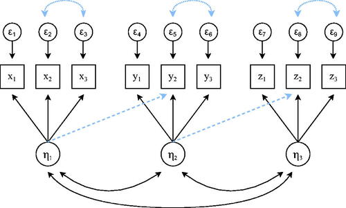
Figure 1. Visualization of imposed structural misspecifications. Misspecification occurs when factor loadings (dashed lines) or residual variances (dotted lines) are present in the population model but not in the analysis model. For each factor, the population values for the factor variance and factor loadings were set to unity and 1, 0.9 and 0.8, respectively. The remaining parameters differed across settings as they were chosen to yield the desired reliability, factor correlation, and misspecification (either zero or 0.2 in standardized terms). A full overview of population values per scenario can be found in our OSF repository.

For each data set, the model parameters were estimated via ML (default), bounded ML (MLB), and all non-iterative methods under consideration: Multiple Group, FABIN2 – ULS, FABIN2 – WLS, FABIN3 – ULS, FABIN3 – WLS, Bentler – ULS, Bentler – WLS, MIIV-2SLS, JS scaling, and JS aggregated. Performance of the different estimation procedures was evaluated with respect to different outcome measures: (i) non-converging solutions (in case of ML), (ii) inadmissible variances (i.e., Heywood cases), and (iii) Mean Square Error (MSE = variance + bias²).

6. Results

6.1. Complete Data

Convergence failures were defined as those iterations for which the lavInspect function from lavaan flagged that convergence was not reached. This implies that either the nlminb optimizer signaled convergence failure, or that an additional gradient check found that not all elements were near zero. Percentages of converged solutions and negative residual variances for ML are reported in Table 2 (complete data only). Especially in low reliability settings, ML suffered from convergence issues, with failure rates up to almost thirty percent for the smallest sample size. Constraining the parameter estimates effectively resolved these issues, as convergence failures for MLB were rare ($<1\%$ across settings). Also with respect to Heywood cases, a substantial percentage of inadmissible solutions were observed for ML. None of the other methods yielded negative variances, except for MIIV-2SLS. The fact that MIIV-2SLS shows similar behavior to ML w.r.t. Heywood cases was to be expected, as the “MIIVsem” package finds the variance parameters by optimizing the ML fit function.

Table 2. Percentages of convergence and negative residual variances observed for ML (complete data) across sample sizes (n = 20, 50, 100, 1000), structural misspecifications (none, omitted loadings, omitted residual covariances), reliabilities (0.8, 0.5), distributions (normal, non-normal), and interfactor correlations (0.4, 0.1).

			Reliability = 0.80				Reliability = 0.50
			Normal (%)		Non-normal (%)		Normal (%)		Non-normal (%)
Outcome	N	Misspecification	cor = 0.4	cor = 0.1	cor = 0.4	cor = 0.1	cor = 0.4	cor = 0.1	cor = 0.4	cor = 0.1
Convergence	20	None	99.89	99.83	99.26	98.27	83.35	74.72	80.73	70.64
		Loadings	99.82	99.71	99.25	97.43	86.10	75.05	83.13	70.11
		Covariances	99.92	99.84	99.26	98.56	85.34	78.16	82.29	74.00
	50	None	100.00	100.00	100.00	100.00	99.66	98.83	99.08	95.80
		Loadings	100.00	100.00	100.00	99.98	99.66	98.09	99.30	95.00
		Covariances	100.00	100.00	100.00	100.00	99.70	99.23	99.02	97.19
	100	None	100.00	100.00	100.00	100.00	100.00	100.00	99.99	99.94
		Loadings	100.00	100.00	100.00	100.00	100.00	99.98	99.99	99.85
		Covariances	100.00	100.00	100.00	100.00	100.00	100.00	100.00	99.93
	1000	None	100.00	100.00	100.00	100.00	100.00	100.00	100.00	100.00
		Loadings	100.00	100.00	100.00	100.00	100.00	100.00	100.00	100.00
		Covariances	100.00	100.00	100.00	100.00	100.00	100.00	100.00	100.00
Heywoods	20	None	2.44	2.70	4.01	4.52	7.10	9.37	7.97	10.06
		Loadings	3.16	3.24	4.76	5.21	6.53	9.36	7.47	10.13
		Covariances	2.73	3.03	4.47	4.92	7.28	9.22	8.18	10.00
	50	None	0.04	0.04	0.23	0.29	0.63	1.47	1.05	2.44
		Loadings	0.23	0.13	0.73	0.57	0.77	2.01	1.23	3.00
		Covariances	0.10	0.14	0.47	0.60	0.83	1.73	1.47	2.71
	100	None	0.00	0.00	0.00	0.00	0.01	0.06	0.05	0.20
		Loadings	0.01	0.00	0.11	0.03	0.04	0.23	0.13	0.57
		Covariances	0.00	0.00	0.01	0.02	0.01	0.13	0.10	0.34
	1000	None	0.00	0.00	0.00	0.00	0.00	0.00	0.00	0.00
		Loadings	0.00	0.00	0.00	0.00	0.00	0.00	0.00	0.00
		Covariances	0.00	0.00	0.00	0.00	0.00	0.00	0.00	0.00

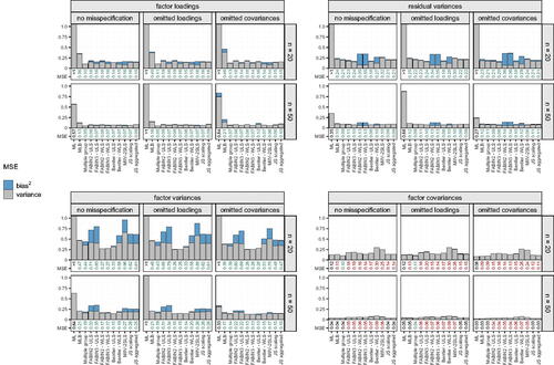
A visual representation of MSE values in a subset of the simulation scenarios (i.e., complete data, no structural misspecification) is found in Figures 2 and 3, where digits show absolute MSE values (averaged across parameters within the group), and colors represent its size relative to ML. To allow for a fair comparison between ML and the other methods under evaluation, only data sets for which ML reached convergence were considered. Although the relative ranking among methods tends to be highly dependent on the specific setting, as well as the parameter type under evaluation (i.e., factor loadings, residual variances, factor (co)variances), a few general observations are worth mentioning. First, w.r.t. the factor loadings and residual variances, all methods perform well: MSE values are always lower or comparable to those for ML, with largest improvements in low reliability settings. In small samples, the same holds for factor variances. Results are, however, less clear-cut for the factor covariances. With already low MSE values for ML, the bulk of the procedures tends to slightly increase – rather than decrease – MSE values. One exception is the Multiple Group method, which shows lower or comparable MSE values across all parameters in all investigated settings. Note, however, that for most methods with higher MSE values (including MLB), the magnitude of the inflation is still fairly limited, especially when compared to the drop in MSE value for other parameters (Figure 4). From the same figure, we can further infer that patterns are highly similar across structural misspecifications.

Figure 2. Overview of MSE values for factor loadings and residual covariances in a subset of the simulation scenarios (complete data, no misspecification). Cell values show MSE values; cell colors represent its size relative to ML (i.e., colors move from white towards blue or orange as they become smaller or larger relative to ML).

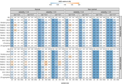
Figure 3. Overview of MSE values for factor (co)variances in a subset of the simulation scenarios (complete data, no misspecification). Cell values show MSE values; cell colors represent its size relative to ML (i.e., colors move from white towards blue or orange as they become smaller or larger relative to ML).

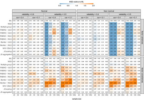
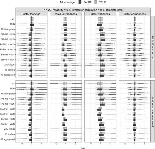
Figure 4. Visualization of average MSE values in a subset of the simulation scenarios (complete normal data, reliability = 0.5, factor correlation = 0.1) for different sample sizes (n = 20, 50). Bars represent MSE values (MSE = variance + bias²), split up by the contribution of variance (gray) and bias squared (blue). The exact MSE value is found below each bar, with the color of the digit indicating whether it is better (green), worse (red) or equal (black) relative to the one observed for ML.

Recall that for all MSE results mentioned above, data sets for which ML did not reach convergence were discarded for all methods. Yet, an apparent asset of non-iterative methods is that they always provide solutions, even when ML does not. In order to be useful alternatives in case of convergence failure, it is important that also for these data sets, sensible estimates are obtained. In general, non-convergence rates were considered too small to extensively evaluate performance in each of the simulation scenarios, but a quick glance into the bias distributions for some of the low convergence settings suggests that this is indeed the case (Figure 5). Although it is important to bear in mind that the boxes for ML convergence failure only draw upon a limited number of data sets, we conclude that they do not raise immediate concern as the bulk of the bias distributions are located at sensible distances from zero.

Figure 5. Boxplots of parameter bias in two simulation settings with low convergence rates, grouped per parameter type. Light and dark boxes represent observed bias for data sets where ML did and did not converge, respectively.

6.2. Missing data

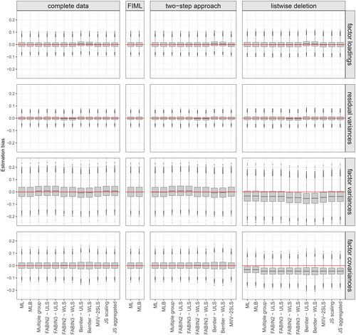
As expected, partial deletion of data resulted in slightly less favorable percentages across all outcome measures (i.e., less convergence, more Heywoods, higher MSE). It did not, however, affect the relative performance of the different estimation procedures under consideration (i.e., highly similar patterns across missingness scenarios). As evident from Figure 6, listwise deletion resulted in biased estimates of factor (co)variances for all methods. This was not the case for estimates obtained from a two-step approach, showing very similar behavior to the complete data setting.

Figure 6. Boxplots of observed bias for different parameters (factor loading, residual variance, factor variance, factor covariance) in favorable circumstances (n = 1000, normal data, no misspecifications, reliability = 0.8, factor correlation = 0.1) across different missingness scenarios (no missingness, FIML, two-step approach, listwise deletion).

7. Discussion

After specifying a factor-analytic model, researchers typically resort to Maximum Likelihood to estimate the model parameters. In ideal circumstances where all of the underlying assumptions are tenable, the desirable statistical properties of the estimator are able to justify this choice. In practice, however, real-life data frequently stretch the limits of the estimation procedure, to the point where iterative minimization of the ML fit function may fail to deliver. When dealing with small samples, for instance, final estimates are frequently biased, inadmissible, or simply unavailable due to convergence failure. In this study, we empirically evaluated various non-iterative methods from which we knew that they would solve at least part of these issues, but have only received limited attention in the past. Aiming for a thorough comparison, we included both old and more recently proposed methods.

Results from our simulation study corroborate previous findings (see, for instance, Stuive, 2007), suggesting that non-iterative procedures may serve as viable alternatives for ML. Whereas ML frequently fails to provide a stable solution, closed-form expressions do not suffer from convergence issues. Evidently, non-iterative estimators are not immune to all conceivable issues, but the source of the problem is usually more readily identifiable, and perhaps even remediable (e.g., when a matrix should be positive definite, solutions exist when this requirement is not met; see Fuller, 1987). Note, however, that the attractiveness of non-iterative procedures in small to moderate samples goes beyond ML’s convergence issues, as the non-iterative methods also frequently outperformed ML in terms of MSE. Among non-iterative procedures, Multiple Group was found most promising as it consistently yielded favorable results across all parameters and settings.

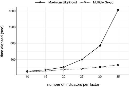
Whereas the current research was constrained to relatively small samples, it would be interesting to examine how they perform at the other end of the spectrum, i.e., when dealing with big and/or high-dimensional data. Especially when the number of indicators grow larger, ML becomes increasingly computationally intensive, and may seriously slow down the analyses. As a proof of concept, we fitted a series of models with an increasing number of indicators with both ML and Multiple Group. Results from a small benchmark pilot shows that the average computation time for ML quickly builds up (see Appendix B). Especially when being used in combination with resampling procedures, resorting to simple closed-form expressions may save researchers several hours, days, or even weeks, without necessarily having to compromise on parameter recovery.

Apart from solving the aforementioned issues and inconveniences, we foresee a an additional setting where closed-form expressions might be of use: the estimation of Structural Equation Models (SEMs) via a Structural After Measurement (SAM) approach (Rosseel & Loh, 2022). Although most of the aforementioned methods are concerned with factor-analytic measurement models and do not incorporate directed relationships among latent variables, they can still be employed in the estimation of SEMs by compartmentalization of the full model into separate measurement blocks. After the measurement blocks have been estimated via non-iterative estimation procedures, remaining parameters can be obtained by considering the measuring parts as fixed (global SAM), or by estimating the mean vector and covariance matrix of the latent variables from the observed summary statistics and the estimates of the measurement parts, and then again using non-iterative approaches (OLS/2SLS) to estimate the structural part (local SAM). These, and other potential uses of non-iterative methods require further investigation, and we hope that the promising results from this research might spark some renewed interest within the field.

Additional information

Funding

This research was supported by a grant of the Ghent University Special Research Fund, grant number BOF.24Y.2019.0011.01.

Appendix A.

 Population model numerical example

$$\mathbf{\Lambda }=\left[\begin{array}{ccc}1.00& 0.00& 0.00\\ 0.80& 0.00& 0.00\\ 0.70& 0.00& 0.00\\ 0.00& 1.00& 0.00\\ 0.00& 0.80& 0.00\\ 0.00& 0.70& 0.00\\ 0.00& 0.00& 1.00\\ 0.00& 0.00& 0.80\\ 0.00& 0.00& 0.70\end{array}\right]\hspace{0.17em}\mathbf{\Theta }=\left[\begin{array}{ccc}1.00& & \\ & \ddots & \\ & & 1.00\end{array}\right]\hspace{0.17em}\mathbf{\Psi }=\left[\begin{array}{ccc}1.00& 0.50& 0.50\\ 0.50& 1.00& 0.50\\ 0.50& 0.50& 1.00\end{array}\right]$$

Appendix B.

 Computation time ML versus multiple group

Figure B1. Results from a small benchmark pilot (1000 replications), comparing the time elapsed for fitting models with an increasing number of indicators per factor with ML (dark, solid) and Multiple Group (light, dotted). Only as a proof of concept; full R code including all model specifications can be found in our OSF repository.

References

- Bentler, P. M. (1982). Confirmatory factor analysis via noniterative estimation: A fast, inexpensive method. Journal of Marketing Research, 19, 417–424. https://doi.org/10.1177/002224378201900403
- Bollen, K. A. (1989). Structural equations with latent variables (vol. 210). John Wiley & Sons.
- Bollen, K. A. (1996). An alternative two stage least squares (2sls) estimator for latent variable equations. Psychometrika, 61, 109–121. https://doi.org/10.1007/BF02296961
- Boomsma, A. (1985). Nonconvergence, improper solutions, and starting values in lisrel maximum likelihood estimation. Psychometrika, 50, 229–242. https://doi.org/10.1007/BF02294248
- Boyer, L., Bastuji-Garin, S., Chouaid, C., Housset, B., Le Corvoisier, P., Derumeaux, G., Boczkowski, J., Maitre, B., Adnot, S., & Audureau, E. (2018). Are systemic manifestations ascribable to copd in smokers? a structural equation modelling approach. Scientific Reports, 8, 1–8. https://doi.org/10.1038/s41598-018-26766-x
- Browne, M. W. (1974). Generalized least squares estimators in the analysis of covariance structures. South African Statistical Journal, 8, 1–24. https://doi.org/10.1002/j.2333-8504.1973.tb00197.x
- Burghgraeve, E., De Neve, J., & Rosseel, Y. (2021). Estimating structural equation models using James–Stein type shrinkage estimators. Psychometrika, 86, 96–130. https://doi.org/10.1007/s11336-021-09749-2
- Cronbach, L. J. (1951). Coefficient alpha and the internal structure of tests. Psychometrika, 16, 297–334. https://doi.org/10.1007/BF02310555
- Cudeck, R. (1991). Noniterative factor analysis estimators, with algorithms for subset and instrumental variable selection. Journal of Educational Statistics, 16, 35–52. https://doi.org/10.3102/10769986016001035
- De Jonckere, J., & Rosseel, Y. (2022). Using bounded estimation to avoid nonconvergence in small sample structural equation modelling. Structural Equation Modelling, 29, 412–427. https://doi.org/10.1080/10705511.2021.1982716
- Devlieger, I., Talloen, W., & Rosseel, Y. (2019). New developments in factor score regression: Fit indices and a model comparison test. Educational and Psychological Measurement, 79, 1017–1037. https://doi.org/10.1177/0013164419844552
- Enders, C. K. (2001). A primer on maximum likelihood algorithms available for use with missing data. Structural Equation Modelling, 8, 128–141. https://doi.org/10.1207/S15328007SEM0801_7
- Fisher, Z., Bollen, K., Gates, K., Rönkkö, M. (2021). Miivsem: Model implied instrumental variable (miiv) estimation of structural equation models [Computer software manual]. https://CRAN.R-project.org/package=MIIVsem (R package version 0.5.8)
- Fuller, W. A. (1987). Measurement error models. John Wiley & Sons.
- Grønneberg, S., Foldnes, N., & Marcoulides, K. M. (2022). Covsim: An R package for simulating non-normal data for structural equation models using copulas. Journal of Statistical Software, 102, 1–45. https://doi.org/10.18637/jss.v102.i03
- Guttman, L. (1944). General theory and methods for matric factoring. Psychometrika, 9, 1–16. https://doi.org/10.1007/BF02288709
- Guttman, L. (1952). Multiple group methods for common-factor analysis: Their basis, computation, and interpretation. Psychometrika, 17, 209–222. https://doi.org/10.1007/BF02288783
- Hägglund, G. (1982). Factor analysis by instrumental variables methods. Psychometrika, 47, 209–222. https://doi.org/10.1007/BF02296276
- Hägglund, G. (1985). Factor analysis by instrumental variables methods: The confirmatory case. University of Uppsala, Department of Statistics.
- Harman, H. H. (1954). The square root method and multiple group methods of factor analysis. Psychometrika, 19, 39–55. https://doi.org/10.1007/BF02288992
- Harman, H. H. (1976). Modern factor analysis (3rd ed.). University of Chicago press.
- Holzinger, K. J. (1944). A simple method of factor analysis. Psychometrika, 9, 257–262. https://doi.org/10.1007/BF02288737
- Horst, P. (1937). A method of factor analysis by means of which all coordinates of the factor matrix are given simultaneously. Psychometrika, 2, 225–236. https://doi.org/10.1007/BF02287894
- Ihara, M., & Kano, Y. (1986). A new estimator of the uniqueness in factor analysis. Psychometrika, 51, 563–566. https://doi.org/10.1007/BF02295595
- Jennrich, R. I. (1987). Tableau algorithms for factor analysis by instrumental variable methods. Psychometrika, 52, 469–476. https://doi.org/10.1007/BF02294367
- Kirby, J. B., & Bollen, K. A. (2009). 10 Using instrumental variable tests to evaluate model specification in latent variable structural equation models. Sociological Methodology, 39, 327–355. https://doi.org/10.1111/j.1467-9531.2009.01217.x
- Kochenderfer, M. J., & Wheeler, T. A. (2019). Algorithms for optimization. Mit Press.
- Little, R. J., & Rubin, D. B. (2019). Statistical analysis with missing data (vol. 793). John Wiley & Sons.
- Lussier, P., LeBlanc, M., & Proulx, J. (2005). The generality of criminal behavior: A confirmatory factor analysis of the criminal activity of sex offenders in adulthood. Journal of Criminal Justice, 33, 177–189. https://doi.org/10.1016/j.jcrimjus.2004.12.009
- Madansky, A. (1964). Instrumental variables in factor analysis. Psychometrika, 29, 105–113. https://doi.org/10.1007/BF02289693
- Nestler, S. (2014). How the 2 sls/iv estimator can handle equality constraints in structural equation models: A system-of-equations approach. British Journal of Mathematical and Statistical Psychology, 67, 353–369. https://doi.org/10.1111/bmsp.12023
- Newman, D. A. (2014). Missing data: Five practical guidelines. Organizational Research Methods, 17, 372–411. https://doi.org/10.1177/1094428114548590
- R Core Team. (2022). R: A language and environment for statistical computing [Computer software manual]. https://www.R-project.org/
- Rosseel, Y. (2012). lavaan: An R package for structural equation modelling. Journal of Statistical Software, 48, 1–36. https://doi.org/10.18637/jss.v048.i02
- Rosseel, Y., & Loh, W. W. (2022). A structural after measurement approach to structural equation modelling. Psychological Methods. https://doi.org/10.1037/met0000503
- Rubin, D. B. (1987). Multiple imputation for nonresponse in surveys (vol. 81). John Wiley & Sons.
- Sargan, J. D. (1958). The estimation of economic relationships using instrumental variables. Econometrica, 26, 393–415. https://doi.org/10.2307/1907619
- Savalei, V., & Bentler, P. M. (2009). A two-stage approach to missing data: Theory and application to auxiliary variables. Structural Equation Modelling, 16, 477–497. https://doi.org/10.1080/10705510903008238
- Savalei, V., & Falk, C. F. (2014). Robust two-stage approach outperforms robust full information maximum likelihood with incomplete nonnormal data. Structural Equation Modelling, 21, 280–302. https://doi.org/10.1080/10705511.2014.882692
- Silvey, S. D. (2017). Statistical inference. Routledge.
- Spearman, C. (1904). ”General intelligence,” objectively determined and measured. The American Journal of Psychology, 15, 201–293. https://doi.org/10.2307/1412107
- Stuive, I. (2007). A comparison of confirmatory factor analysis methods: Oblique multiple group method versus confirmatory common factor method [Ph.D. thesis]. University of Groningen.
- Takane, Y., & Hwang, H. (2018). Comparisons among several consistent estimators of structural equation models. Behaviormetrika, 45, 157–188.
- Thurstone, L. L. (1945). A multiple group method of factoring the correlation matrix. Psychometrika, 10, 73–78. https://doi.org/10.1007/BF02288876
- Toyoda, H. (1997). A noniterative estimation in confirmatory factor analysis by an instrumental variable method. Behaviormetrika, 24, 147–158. https://doi.org/10.2333/bhmk.24.147
- van Buuren, S., & Groothuis-Oudshoorn, K. (2011). Mice: Multivariate imputation by chained equations in r. Journal of Statistical Software, 45, 1–67.
- Yu, H., Campbell, M. T., Zhang, Q., Walia, H., & Morota, G. (2019). Genomic Bayesian confirmatory factor analysis and Bayesian network to characterize a wide spectrum of rice phenotypes. Genes, Genomes, Genetics, 9, 1975–1986.