Exploratory Factor Analysis Trees: Evaluating Measurement Invariance Between Multiple Covariates

Abstract

Measurement invariance (MI) describes the equivalence of a construct across groups. To be able to meaningfully compare latent factor means between groups, it is crucial to establish MI. Although methods exist that test for MI, these methods do not perform well when many groups have to be compared or when there are no hypotheses about them. We suggest a method called Exploratory Factor Analysis Trees (EFA trees) that are an extension to SEM trees. EFA trees combine EFA with a recursive partitioning algorithm that can uncover non-invariant subgroups in a data-driven manner. An EFA is estimated and then tested for parameter instability on multiple covariates (e.g., age, education, etc.) by a decision tree based method. Our goal is to provide a method with which MI can be addressed in the earliest stages of questionnaire development or prior to analyses between groups. We show how EFA trees can be implemented in the software R using lavaan and partykit. In a simulation, we demonstrate the ability of EFA trees to detect a lack of MI under various conditions. Our online material contains a template script that can be used to apply EFA trees on one’s own questionnaire data. Limitations and future research ideas are discussed.

Keywords:

• Decision trees
• exploratory factor analysis
• measurement invariance
• recursive partitioning

1. Introduction

In psychometrics, measurement invariance (MI) describes the equivalence of measurements of a construct across groups (Putnick & Bornstein, 2016; Vandenberg & Lance, 2000). This concerns different groups of a population (e.g., women and men) or subsequent measurement occasions of the same group (e.g., pre- and post-treatment). If MI does not hold between two or more groups, it cannot be readily assumed that the construct of interest has the same meaning to people between these groups. Consequently, analyses like comparisons of means and variances across groups or measurement occasions will not be meaningful or will even yield distorted results. Multi-group confirmatory factor analysis (MG-CFA) is one of the most commonly used methods to test for MI (Millsap, 2012). However, it is mostly used for comparing two groups. When comparing many groups, the performance of MG-CFA is reduced because the number of measurement parameters to pairwisely compare increases exponentially with the number of groups and non-invariance is falsely detected more easily (Kim et al., 2017; Rutkowski & Svetina, 2014). Additionally, researchers have to determine the groups or at least the grouping variable a priori (e.g., age or gender; in the following called covariates) (Kim et al., 2017). This often happens with a special application in mind (e.g., cross-cultural comparisons; Milfont & Fischer, 2010) and is mostly done for questionnaires that have already been constructed. We argue that MI should ideally be addressed in the earliest stages of questionnaire development, when changes to the item pool are still easily possible. To address this issue, we want to introduce a method that can help researchers to explore MI in their sample and to automatically identify non-invariant groups: exploratory factor analysis trees (EFA trees). EFA trees can be seen as an extension of structural equation model (SEM) trees introduced by Brandmaier et al. (2013b). SEM trees combine SEM with a recursive partitioning algorithm. A SEM is estimated and then tested for parameter instability by a decision tree based method. Thereby, they allow for testing for MI with regard to categorical and continuous covariates (Brandmaier et al., 2013a). This is done in a data-driven manner, that is, no covariate has to be chosen in advance. Although decision trees and, thus, SEM trees are already exploratory in nature, so far SEM trees have mainly been applied in the context of CFA or to longitudinal data but to the best of our knowledge not in the context of EFA (Ammerman et al., 2019; Brandmaier et al., 2016, 2017, 2018; de Mooij et al., 2018; Simpson-Kent et al., 2020; Usami et al., 2017, 2019). By introducing EFA trees, we want to extend the SEM tree literature and provide researchers with an easy-to-use method that grasps the full exploratory potential of SEM trees (Goretzko & Bühner, 2022; Jacobucci et al., 2017). We illustrate how EFA trees can be built within the partykit R package (Hothorn & Zeileis, 2015) that provides tools for model-based recursive partitioning (Hothorn et al., 2006; Zeileis et al., 2008).

The remainder of the paper is structured as follows. First, we describe the concept of MI and its relevance for questionnaire development in more detail. Second, we provide an introduction to EFA. Third, we describe the recursive partitioning algorithm and EFA trees in particular. Last, we show exemplary applications of EFA trees and investigate the performance in identifying a lack of MI under different conditions in simulated examples.

2. Measurement Invariance

Assessing MI can be a tedious task. In a factor-analytic framework, four nested levels of MI between groups are considered (Putnick & Bornstein, 2016): a) configural (equal construct architecture; i.e., same number of latent factors and same location of zero loadings in the loading matrices across groups. Note that zero loadings are only imposed in CFA, not in EFA.), b) metric (equal loading sizes), c) scalar (equal intercepts), d) residual (equal unique variance). As already mentioned, MG-CFA is a straightforward way to test for MI (see Putnick & Bornstein, 2016 for an illustrative step-by-step example). However, if there are many groups that have to be compared, this simple approach reaches its limits. The probability of falsely detecting non-invariance increases with number of groups to be compared and model fit might be poor due to strict fit index cut offs (Kim et al., 2017). Rutkowski and Svetina (2014) provided a first remedy to tackle this issue by suggesting adapted cut-offs for model fit measures. Even further, scholars developed other CFA-based methods to test MI in these cases with many groups, for example multilevel factor mixture modelling or alignment optimization (Asparouhov & Muthén, 2014). Because going into detail about these methods would be beyond the scope of this article, we refer readers interested in CFA-based methods to Kim et al. (2017) for a comprehensive overview. Sass (2011) and Van de Schoot et al. (2012) provide general guidelines on testing for MI.

In addition to these CFA-based methods, other EFA-based methods have been developed recently. This resolves some of the aforementioned issues, for example that no restrictive zero loadings have to be imposed. For example, De Roover and Vermunt (2019) developed multigroup factor rotation to pinpoint non-invariant loadings between groups. Mixture multigroup factor analysis was suggested as a method to cluster groups according to levels of MI, specifically metric (De Roover et al., 2022) and scalar (De Roover, 2021) invariance.

Even though some of these advanced methods can handle many groups, problems arise when there are no particular hypotheses with regard to the covariates defining these groups (Brandmaier et al., 2013b). When there are many covariates (e.g., age, gender, education, ethnicity, etc.), it quickly becomes impossible to test for all of them with all potential group constellations. Usually when researchers test for MI, they define a small number of groups based on one or two covariates (e.g., ethnicity in cross-cultural research). In this, other covariates (or interactions between them) that may define theoretically relevant groups and for which MI cannot be assumed might remain undetected. As Brandmaier et al. (2013b) described, SEM trees can be used to explore the data for non-invariant groups in a data-driven manner (rather than by theoretically deriving hypotheses a priori). Thus, the concept of recursive partitioning seems suitable for exploration of MI with many covariates. To expand this potential to the earliest stages of questionnaire development, we extend SEM trees by EFA trees. Our aim is to add a method to the tool box that can aid researchers in exploring and testing for MI in order to develop questionnaires that considered MI right from the start. Admittedly, this will not render tests for MI prior to actual analyses between two or more defined groups unnecessary. However, EFA trees may improve the measurement quality of psychological constructs and hopefully prevent later issues with data collection and analysis (Jacobucci & Grimm, 2020).

3. Exploratory Factor Analysis

EFA is arguably one of the most widely used methods in psychometrics and questionnaire development more specifically. Compared to CFA, there are no constraints on loading paths between the observed variables and the latent factors. Hence, EFA can be used to uncover the relationships between observed and latent variables (Goretzko et al., 2021; Mulaik, 2010). More formally, let $\mathit{x}={(x_1,\dots ,x_p)}^{\top }$ be the p-dimensional vector of observed variables. This vector can be described as a linear function of the m latent factors (Hirose & Yamamoto, 2014; Mulaik, 2010): (1) $$\mathit{x}=\mathit{\tau }+\mathbf{\Lambda }\mathit{\xi }+\mathit{ϵ}$$(1) where $\mathit{\tau }={({\tau }_1,\dots ,{\tau }_p)}^{\top }$ is the p-dimensional vector of intercepts, $\mathbf{\Lambda }$ is the $p\times m$ matrix of factor loadings, $\mathit{\xi }={({\xi }_1,\dots ,{\xi }_m)}^{\top }$ is the m-dimensional vector of latent factor scores, and $\mathit{ϵ}={({ϵ}_1,\dots ,{ϵ}_p)}^{\top }$ is the p-dimensional vector of error terms of the observed variables. The error terms are assumed to be normally distributed with mean 0 and variance $\mathbf{\Psi }.$ $\mathbf{\Psi }$ is a $p\times p$ diagonal matrix with the diagonal elements being the unique variances of the observed variables. The factor correlations are captured as the elements of the $m\times m$ matrix $\mathbf{\Phi }.$ In EFA, the factors have rotational freedom, that is, there exist different sets of factor solutions which have an identical fit to the data but might be easier to interpret. We resolve the issue of rotational freedom by using regularization (an explanation will follow in a later section). The vector $\mathit{x}$ is usually assumed to be multivariate-normally distributed with mean vector $\mathit{\tau }$ and variance-covariance matrix $\mathbf{\Sigma }=\mathbf{\Lambda }\mathbf{\Phi }{\mathbf{\Lambda }}^{\top }+\mathbf{\Psi }$ (Jöreskog, 1967). In the single-group context, the data are usually standardized so that $\mathit{\tau }=0$ and $\mathit{diag}(\mathbf{\Sigma })=1.$ In the multi-group context, it is common to keep the data unstandardized and instead use the covariance matrices for model estimation.

We later want to understand how EFA trees detect measurement non-invariance. For this, we have to introduce an estimation function with which the model parameters (i.e., factor loadings, factor correlations, and unique variances) are estimated. The algorithm uses maximum likelihood estimation (MLE). In MLE, parameters are estimated so that the discrepancy between the model-implied covariance matrix $\mathbf{\Sigma }$ and the observed covariance matrix $\mathit{S}$ is minimized (Jöreskog, 1967): (2) $$F_{\mathit{MLE}}(\mathbf{\Sigma },\mathbf{S})=\hspace{0.17em}\ln \hspace{0.17em}\left|\mathbf{\Sigma }\right|+tr({\mathbf{\Sigma }}^{-1}\mathit{S})-\hspace{0.17em}\ln \hspace{0.17em}\left|\mathit{S}\right|-p.$$(2)

MLE has some convenient properties (Fabrigar et al., 1999): In the estimation process, standard errors of the model parameters are computed. These can be used to calculate confidence intervals and assess the statistical significance of factor loadings¹. Additionally, fit indexes (e.g., RMSEA, CFI, etc.) can be computed that are useful for model evaluation and comparison.

4. Score-Based Recursive Partitioning

Now that we have elaborated on how the EFA model is estimated, we turn to the score-based recursive partitioning algorithm (Hothorn et al., 2006; Zeileis et al., 2008). Specifically, how the algorithm finds parameter instability in the model with respect to some covariate and splits the data into heterogeneous groups. The algorithm is based on a tree structure common in machine learning. In detail, the algorithm works as follows (Hothorn et al., 2006; Zeileis et al., 2008):

1. A model (in our case, an EFA) is fit to the entire sample by estimating the model parameters via MLE (see equation (2)(2) $$F_{\mathit{MLE}}(\mathbf{\Sigma },\mathbf{S})=\hspace{0.17em}\ln \hspace{0.17em}\left|\mathbf{\Sigma }\right|+tr({\mathbf{\Sigma }}^{-1}\mathit{S})-\hspace{0.17em}\ln \hspace{0.17em}\left|\mathit{S}\right|-p.$$(2) ). Let $\Pi (\mathit{Y},\mathit{\theta })$ be the estimation function in equation (2)(2) $$F_{\mathit{MLE}}(\mathbf{\Sigma },\mathbf{S})=\hspace{0.17em}\ln \hspace{0.17em}\left|\mathbf{\Sigma }\right|+tr({\mathbf{\Sigma }}^{-1}\mathit{S})-\hspace{0.17em}\ln \hspace{0.17em}\left|\mathit{S}\right|-p.$$(2) , $\mathit{\theta }=(\mathbf{\Lambda },\mathbf{\Phi },\mathbf{\Psi })$ the vector of model parameters (i.e., factor loadings, factor correlations, and unique variances) and $\mathit{Y}$ the observations, with elements $Y_i,$ $i=1,\dots ,N.$ The parameter estimates $\widehat{\mathit{\theta }}$ can be obtained by solving the first order condition (3) $$\sum _{i=1}^N\pi (Y_i,\widehat{\mathit{\theta }})=0$$(3) whereby (4) $$\pi (\mathit{Y},\mathit{\theta })=\frac{\partial \Pi (\mathit{Y},\mathit{\theta })}{\partial \mathit{\theta }}$$(4) is the score function of $\Pi (\mathit{Y},\mathit{\theta }).$

2. A test for parameter stability is performed with regard to every covariate by means of null hypothesis tests (structural change test). For this, we assess whether the corresponding scores evaluated at the parameter estimates, ${\widehat{\pi }}_i=\pi (Y_i,\widehat{\mathit{\theta }}),$ fluctuate randomly around their mean 0. The scores are ordered according to their deviation from 0 with regard to a covariate. Under the null hypothesis of invariant measurement, the deviations should fluctuate randomly. If, however, the measurement is not invariant, systematic changes in the deviations will be shown by the ordering. The hypothesis tests use different test statistics depending on whether a categorical or continuous covariate is evaluated. In this study, we used a ${\chi }^2$ test for categorical covariates and the supLM statistic (a type of Lagrange Multiplier statistic) for continuous covariates. The model needs to be estimated only once to assess MI with regard to different covariates. This is because the amount of score deviations stays the same, only the ordering changes. After every covariate has been evaluated, the one associated with the lowest (Bonferroni-corrected) p-value below a significance level $\alpha$ is selected for splitting the model. Note that by Bonferroni-correcting the p-values, the prespecified significance level $\alpha$ is ensured for the whole tree and the issue of multiple testing is accounted for.

3. Once a covariate for splitting is found, the optimal split point on this covariate has to be computed. When splitting the model into B segments, two potential segmentations can be compared by evaluating the segmented estimation functions ${\sum }_{b=1}^B\sum _{i\in I_b}\Pi (Y_i,{\mathit{\theta }}_b).$ For continuous covariates, an exhaustive search over all potential segmentations is performed. For a split into $B=2$ segments, this can be performed in $O(N)$ operations, where N is the sample size. As an example, suppose the continuous variable age was identified in step 2 as a covariate that explains parameter instability. To find the optimal split point, the algorithm now loops over every value of age from lowest to highest and compares the segmented estimation functions for the groups that would result from splitting at the evaluated value. The value of age for which the two segmented estimation functions are optimized is then selected as the split point. For categorical covariates, all potential constellations are evaluated. For a split into $B=2$ segments, this can be performed in $O(2^{C-1})$ operations, with C being the number of categories. For example, on the categorical variable marital status with four categories, the segmented estimation functions of every group constellation are compared. Again, the constellation for which the estimation functions are optimized is selected for splitting. Theoretically, the model could be split into more than two nodes. However, this diminishes interpretability while simultaneously increasing computational demand (e.g., for continuous variables, a split into more than two groups, $B>2,$ would result in an exhaustive search of order $O(N^{B-1})$). In the following, we only consider the case where the model is split into two nodes (cf. Brandmaier et al., 2013b; Strobl et al., 2015; Zeileis et al., 2008). Note that if there were three non-invariant groups, they could still be identified by performing binary splits. For this, the algorithm would simply split twice on the same covariate.

4. These steps are repeated until a) no parameter instability in a leaf node becomes statistically significant, b) a prespecified depth of the tree is reached, or c) sample size in a leaf node falls below a prespecified minimal value. For a thorough mathematical introduction see Hothorn et al. (2006), Zeileis and Hornik (2007) and Zeileis et al. (2008).

This algorithm has some convincing advantages (Hothorn et al., 2006; Zeileis et al., 2008): First, it is possible to efficiently test multiple covariates for parameter instability, even without hypotheses about split points. This is especially powerful in the case of continuous covariates like age where manually assessing every potential split point is not feasible (Putnick & Bornstein, 2016). Second, (non-linear) interactions between covariates can be considered. This can be done either by adding the interaction term as a potential covariate or by allowing “deeper” trees. Nodes are conditional on all prior covariates and split points. Hence, in a tree that was split twice on two different covariates, these can be seen as an interaction. Third, the algorithm is unbiased. Other tree algorithms (like CART or C4.5) often tend to favor covariates with many potential split points and are thus biased toward selecting these covariates for splitting. In the score-based recursive partitioning algorithm, this selection bias is eliminated by separating the steps of covariate selection and split point selection. Additionally, the algorithm works on formal parameter stability tests, which also ensures unbiasedness. That is, if the parameters in a node are stable, a false decision to split on any of the covariates will only be made with a probability of approximately $\alpha .$ Conversely, if the parameters are in fact unstable, and this instability can be explained by a covariate, the instability will be detected for a sufficient sample size N. This is because the tests are consistent at rate $\sqrt{N}$ (Zeileis & Hornik, 2007).

We want to point out that using this recursive partitioning approach is not new in psychometrics and has repeatedly shown good performance. In recent years, it was primarily employed to models in the IRT framework like dichotomous (Strobl et al., 2015) and polytomous (Komboz et al., 2018) Rasch models. They can be used to detect differential item functioning (DIF; Holland & Wainer, 2012) between multiple covariates (Debelak & Strobl, 2019). Schneider et al. (2021) provide a tutorial on score-based MI tests in IRT models. We want to extend this literature by combining recursive partitioning with EFA. This might be especially useful for complex constructs where multiple scales ought to be tested for MI simultaneously (Meade & Lautenschlager, 2004). Merkle and Zeileis (2013) and Merkle et al. (2014) introduced this algorithm in a factor-analytic context. Their work evaluated the performance of the statistical tests used in our study and thus prepared the technical ground on which our study is built. Both of their studies focused on comparing different test statistics for continuous (Merkle & Zeileis, 2013) and ordinal (Merkle et al., 2014) covariates. We aim to add to this literature by carrying the method to typical psychological research situations. We hope to provide a broader context, for example by considering different violations of MI and types of covariates at the same time. In this, we want to enable substantive researchers to draw on a well-known and commonly used method in psychological questionnaire development when evaluating MI (Fabrigar et al., 1999; Goretzko et al., 2021). This could be especially useful in areas like personality or clinical psychology where constructs are often multi-dimensional.

5. EFA Trees

The main purpose of EFA trees is to help researchers to develop questionnaires and psychological tests that have been constructed as measurement invariant as possible. Once a preliminary item set has been built and data have been collected, EFA trees can be used to automatically uncover heterogeneous groups with regard to multiple covariates. In this, EFA trees can be seen as fully exploratory.

The focus of the succeeding simulations will be on detecting a lack of configural and metric MI (Putnick & Bornstein, 2016; Vandenberg & Lance, 2000). That is, we will primarily investigate the ability of EFA trees to assess the construct architecture (i.e., number of latent factors and location of zero loadings) and loading sizes across groups. The two other types of MI, namely scalar (intercept) and residual (unique variances) MI, build on configural and metric MI. Because in EFA data are most often standardized, the mean vector $\tau$ becomes 0 and will not be relevant anymore. Additionally, having equal unique variances across groups is hard to achieve and not necessary for a comparison of latent means (Chen, 2007; Putnick & Bornstein, 2016; Vandenberg, 2002).

We investigated whether a lack of MI is actually detected by EFA trees. For this, we first performed four simulations which act as toy examples. In these, we aimed at demonstrating the application and interpretation of EFA trees to questionnaire data. Subsequently, we conducted a comprehensive simulation study in which we manipulated sample size, group size ratio, type of covariate, number of distraction covariates, and type of lack of MI.

6. Method

6.1. Software

The complete code needed to reproduce all analyses can be found at https://osf.io/7pgrb/. Additionally, we provide a template script which can be used to run an EFA tree with only small adjustments to the code. We conducted all analyses using the statistical software R (R Core Team, 2021). The manuscript was written in R markdown using the package papaja (Aust & Barth, 2020). We simulated standardized data by drawing from a multivariate normal distribution using the package mvtnorm (Genz et al., 2002). The recursive partitioning algorithm was implemented using the package partykit (Hothorn & Zeileis, 2015). In the tree growing function mob, a control argument can be defined that contains parameters relevant for fitting the algorithm. All control parameters were set as their default values. Most importantly, this means that for the significance level for splitting, we set $\alpha =0.05$ and p-values were Bonferroni-corrected. For all analyses, we specified a three-dimensional model with 18 observed variables using the package lavaan (Rosseel, 2012). Every observed variable was allowed to load freely on every factor. Because the recursive partitioning algorithm cannot handle unidentified models, we first defined a model with uncorrelated factors to ensure identification. By setting the argument auto.efa = TRUE in the lavaan function, all constraints to identify a model were imposed: factor correlations were set to 0, factor variances were set to 1, and some factor loadings were constrained to followed an echelon pattern (Rosseel, 2012). Because we assume that no information about the items or the data is available in advance, it is difficult to provide a general recommendation regarding the selection of loadings to constrain. If the wrong loadings are constrained, parameter differences that are critical for the assessment of non-invariance might remain undetected. However, one can empirically assess whether different selections of constrained loadings have a considerable influence (Dolan et al., 2009). This can be done by growing more than one tree in parallel with different constrained loadings and comparing the results.

6.2. Toy Examples

6.2.1. Procedure

The algorithm was employed as described in the section Software. To demonstrate exemplary applications and interpretations of EFA trees, we further investigated the estimated models in the leaf nodes after splitting. For this, we extracted the data from these nodes and re-estimated an unidentified model with correlated factors and all loading paths freed using regularized EFA (Hirose & Yamamoto, 2014; Scharf & Nestler, 2019). We want to briefly explain our rationale behind using regularized EFA: Once the EFA model has been estimated, researchers often aim at obtaining an interpretable solution of the matrix of factor loadings $\mathbf{\Lambda }$ (Mulaik, 2010). The most common goal is to achieve a so-called simple structure. That is, each item has one high loading on one factor and low to no cross-loadings on all other factors. The method of choice to obtain such a structure is rotation of factor solutions. EFA models are rotationally indeterminate, that is, there is an infinite set of factor solutions that fits a data set equally well (Mulaik, 2010). Many rotation methods exist with no one best method (Browne, 2001; Trendafilov, 2014). The best method to use in a specific application depends on the true factor structure in the population. Because this population factor structure is almost always unknown, the choice of rotation method is rather subjective (Asparouhov & Muthén, 2009; Sass & Schmitt, 2010; trying different hyperparameter settings of the simplimax rotation could help to find a solution with most loadings close to zero; see Kiers, 1994 for more details). The very goal of EFA trees is to uncover different structures of a construct between groups. Thus, it is difficult to pick an optimal rotation method for every EFA estimated in a leaf node of the resulting tree². Taking this into account, we applied regularized EFA to obtain interpretable factor solutions in the leaf nodes (Hirose & Yamamoto, 2014; Jacobucci et al., 2016). As Scharf and Nestler (2019) demonstrated in a comprehensive comparison of common rotation methods and regularization, the latter is not necessarily “better” than rotation in recovering simple structure. However, it proves more objective in the sense that the true structure of the construct does not have to be known. Essentially, regularization switches the rotation problem of EFA to a variable selection problem. The regularization was implemented using the package regsem (Jacobucci et al., 2016). We used elastic net regularization (Zou & Hastie, 2005) and penalized both the factor loadings and the factor correlations. The hyperparameters $\gamma$ (controlling the amount of regularization) and $\beta$ (controlling the type of regularization) were tuned by choosing values that minimized the BIC over the whole sample (Jacobucci et al., 2016). For $\gamma ,$ we tested 100 values in a grid search starting from $\gamma =0.001$ with a step size of ${10}^{-5}.$ For $\beta ,$ we tested all values between 0.05 and 0.95 with a step size of 0.05 (cf. Scharf & Nestler, 2019). For regsem, an unidentified model was not an issue because the cv_regsem function only requires the model-implied covariance matrix, not an identified model. In the process of estimation, the model eventually became identified due to variable selection (Li et al., 2021).

6.2.2. Toy Example 1: Configural Invariance - Different Number of Factors

In a first toy example, we investigated whether an EFA tree would detect a violation of configural invariance caused by differing numbers of latent factors between groups. Suppose our construct that was measured by 18 indicators. For men, these indicators were described by three latent factors, whereas for women, there were four latent factors. The standardized loading matrices on population level were (cf. Scharf & Nestler, 2019): $${\mathbf{\Lambda }}_{\mathbf{Men}}=\left[\begin{array}{ccc}0.75& 0& 0\\ 0.75& 0& 0\\ 0.75& 0& 0\\ 0.75& 0& 0\\ 0.75& 0& 0\\ 0.75& 0& 0\\ 0& 0.75& 0\\ 0& 0.75& 0\\ 0& 0.75& 0\\ 0& 0.75& 0\\ 0& 0.75& 0\\ 0& 0.75& 0\\ 0& 0& 0.75\\ 0& 0& 0.75\\ 0& 0& 0.75\\ 0& 0& 0.75\\ 0& 0& 0.75\\ 0& 0& 0.75\end{array}\right];{\mathbf{\Lambda }}_{\mathbf{Women}}=\left[\begin{array}{cccc}0.75& 0& 0& 0\\ 0.75& 0& 0& 0\\ 0.75& 0& 0& 0\\ 0.75& 0& 0& 0\\ 0.75& 0& 0& 0\\ 0& 0& 0& 0.75\\ 0& 0.75& 0& 0\\ 0& 0.75& 0& 0\\ 0& 0.75& 0& 0\\ 0& 0.75& 0& 0\\ 0& 0.75& 0& 0\\ 0& 0& 0& 0.75\\ 0& 0& 0.75& 0\\ 0& 0& 0.75& 0\\ 0& 0& 0.75& 0\\ 0& 0& 0.75& 0\\ 0& 0& 0.75& 0\\ 0& 0& 0& 0.75\end{array}\right]$$

As can be seen, the loading matrices of both men and women did not have cross-loadings. However, the last indicator of each of the three factors in the group of men was shifted to a forth factor in the group of women. We simulated a data set with $N=400$ and the dichotomous covariate sex, consisting of 200 men and 200 women. Additionally, we simulated four covariates as “distractors” to mimic a setting typical for questionnaire development: two (standard-normally distributed) continuous, one other dichotomous, and one categorical covariate with four categories. These covariates were independent from the factorial structure on population level but could have potentially been selected by the EFA tree as a split variable. As described above, we estimated a model with three factors (i.e., a misspecified model for women). In parametric notation, the present violation of configural invariance means that $\Phi$ is a $3\times 3$ matrix for men and a $4\times 4$ matrix for women. The results of the analysis are shown in Table 1. The EFA tree successfully identified the covariate sex for splitting and ignored the four other covariates. Thus, all men and all women ended up in two different leaf nodes. We also conducted a parallel analysis (Horn, 1965) on the data in each leaf node, which correctly suggested three factors in the “male node” and four factors in the “female node.” Especially in the early stages of questionnaire development, a parallel analysis in each leaf node seems beneficial. Table 2 shows the loading matrices of the regularized EFA models in the two leaf nodes. The matrices with the theoretically assumed three latent factors show no clear cause of the violation of MI. However, in the matrix with four latent factors in the female node, as indicated by the data, it can be seen that the observed variables 6, 12, and 18 load on an additional factor not present in the male node. Unfortunately, different number of factors cannot be evaluated directly because the algorithm can only handle one pre-specified model. However, in these cases it would remain unclear anyways what different numbers of latent factors mean on a conceptual level. This emphasizes that further analyses on the data in the leaf nodes are crucial to better understand your data and, ultimately, the construct of interest (cf. Brandmaier et al., 2013b).

Table 1. Test statistics and p-values for toy example 1.

	sex	cov1	cov2	cov3	cov4
statistic	152.45	80.20	122.47	57.43	208.36
p.value	0.00	1.00	0.02	1.00	0.95

Note. Test statistics were a ${\chi }^2$ test for categorical and the supLM statistic for continuous covariates. cov1 - cov4 denote the distractor covariates.

Table 2. Regularized factor solution for toy example 1.

Men			Women 3 Factors			Women 4 Factors
F1	F2	F3	F1	F2	F3	F1	F2	F3	F4
0.72	0.01	0.13	0.73	0.08	0.03	0.72	0.09	0.00	0.03
0.72	0.04	0.07	0.64	0.09	0.03	0.63	0.10	0.01	0.02
0.75	0.00	0.01	0.76	0.00	0.00	0.76	0.00	0.06	−0.02
0.80	0.07	0.01	0.78	−0.03	0.06	0.77	−0.01	−0.02	0.06
0.73	0.06	−0.01	0.68	0.07	0.10	0.67	0.07	0.03	0.10
0.76	0.00	0.00	0.04	0.19	0.23	0.03	0.04	0.68	0.09
0.11	0.72	0.07	0.14	0.72	0.03	0.14	0.72	0.02	0.04
0.00	0.73	0.11	−0.03	0.70	0.10	−0.03	0.71	0.00	0.11
0.11	0.71	−0.04	0.05	0.77	0.04	0.05	0.78	−0.01	0.05
0.04	0.75	0.07	0.06	0.70	0.00	0.06	0.69	0.04	0.00
0.10	0.75	0.00	0.00	0.73	−0.02	0.00	0.69	0.15	−0.04
−0.05	0.77	0.15	0.00	0.22	0.16	0.00	0.07	0.72	0.00
0.13	0.00	0.69	0.00	0.02	0.73	0.00	0.02	0.00	0.74
0.02	0.06	0.73	−0.03	0.00	0.83	−0.03	−0.01	0.08	0.81
0.00	0.16	0.72	0.02	0.05	0.74	0.02	0.06	−0.02	0.75
0.00	0.09	0.71	0.00	0.13	0.75	0.00	0.12	0.07	0.73
0.04	−0.01	0.76	0.02	0.00	0.73	0.02	0.00	0.04	0.72
0.02	0.13	0.71	0.01	0.16	0.26	0.00	0.00	0.70	0.12

Note. F1–F4 denote the latent factors. The factor solutions were achieved by re-estimating the models in the leaf nodes via elastic net regularization.

6.2.3. Toy Example 2: Configural Invariance - Simple Structure vs. Cross-Loadings

In the second toy example, we looked at a different form of configural non-invariance, that is, simple structure in one group and cross-loadings in the other group. We again used the construct with 18 indicators from toy example 1. This time, the number of latent factors was three for both groups. However, the two groups were now defined by a (standardized) continuous covariate age. We simulated the groups based on the z-scores at the mean 0: $z_{\mathit{age}}\le 0$ was the “younger” group and $z_{\mathit{age}}>0$ the “older” group. This yielded approximately equally sized groups. Note that while this leads to two age-groups that have to be uncovered by the EFA tree, it still has to treat age as a continuous variable when assessing parameter instability on this covariate. The standardized loading matrix on population level for the younger group was the same as the one of the men used in toy example 1. For the older group, cross-loadings were added (cf. Scharf & Nestler, 2019): $${\mathbf{\Lambda }}_{\mathbf{Younger}}=\left[\begin{array}{ccc}0.75& 0& 0\\ 0.75& 0& 0\\ 0.75& 0& 0\\ 0.75& 0& 0\\ 0.75& 0& 0\\ 0.75& 0& 0\\ 0& 0.75& 0\\ 0& 0.75& 0\\ 0& 0.75& 0\\ 0& 0.75& 0\\ 0& 0.75& 0\\ 0& 0.75& 0\\ 0& 0& 0.75\\ 0& 0& 0.75\\ 0& 0& 0.75\\ 0& 0& 0.75\\ 0& 0& 0.75\\ 0& 0& 0.75\end{array}\right];{\mathbf{\Lambda }}_{\mathbf{Older}}=\left[\begin{array}{ccc}0.67& 0.22& 0.13\\ 0.68& 0.09& 0.23\\ 0.68& 0.27& 0.05\\ 0.65& 0.39& 0.09\\ 0.64& 0.13& 0.39\\ 0.67& 0.18& 0.18\\ 0.05& 0.68& 0.27\\ 0.28& 0.63& 0.38\\ 0.38& 0.63& 0.21\\ 0.09& 0.69& 0.18\\ 0.05& 0.73& 0.05\\ 0.27& 0.67& 0.13\\ 0.04& 0.40& 0.66\\ 0.38& 0.25& 0.63\\ 0.26& 0.18& 0.66\\ 0.14& 0.09& 0.70\\ 0.22& 0.22& 0.66\\ 0.18& 0.09& 0.69\end{array}\right]$$

${\Lambda }_{\mathit{Older}}$ had its main loadings at the same location as ${\Lambda }_{\mathit{Younger}}$ but had (considerable) cross-loadings (up to 0.4). We simulated a data set with $N=1000$ and the continuous covariate age that defined the two groups as described above. Again, we simulated four distractors: two other (standard-normally distributed) continuous, one dichotomous, and one categorical covariate with four categories. Factor correlations on population level were 0.3, factor variances were fixed to 1. The results are shown in Table 3. The EFA tree identified the covariate age and split the data approximately at $z_{\mathit{age}}=0$ (one observation from the younger group near the mean 0 was falsely put in the leaf node of the older group). It ignored all other covariates. The standardized root mean square residuals (SRMR) of the EFA models in the leaf nodes were 0.01 and 0.01 for the younger and the older group, respectively, indicating good fit. Additionally, regularization of the models in the leaf nodes (approximately) recovered the simple structure in the younger group and the considerable cross-loadings of some observed variables in the older group (see Table 4). This could be considered an indication of configural non-invariance.

Table 3. Test statistics and p-values for toy example 2.

	age	cov1	cov2	cov3	cov4
statistic	474.38	94.96	92.62	67.93	217.60
p.value	0.00	0.90	0.95	0.97	0.82

Note. Test statistics were a ${\chi }^2$ test for categorical and the supLM statistic for continuous covariates. cov1 - cov4 denote the distractor covariates.

Table 4. Regularized factor solution for toy example 2.

Younger			Older
F1	F2	F3	F1	F2	F3
0.76	−0.01	0.01	0.70	0.11	0.11
0.76	0.00	0.00	0.65	0.00	0.29
0.72	0.04	0.06	0.72	0.20	0.00
0.76	0.06	−0.02	0.69	0.30	0.06
0.76	0.04	0.02	0.62	0.00	0.42
0.75	0.11	0.04	0.68	0.11	0.15
−0.06	0.78	0.04	0.00	0.66	0.26
0.01	0.77	0.01	0.27	0.59	0.36
0.00	0.78	0.06	0.42	0.57	0.17
0.01	0.73	0.05	0.11	0.64	0.16
0.05	0.76	0.00	0.05	0.78	−0.06
0.03	0.76	−0.03	0.28	0.65	0.07
0.01	0.00	0.72	−0.03	0.35	0.68
0.04	0.00	0.74	0.31	0.15	0.68
0.05	0.00	0.76	0.19	0.13	0.68
−0.01	0.03	0.72	0.08	0.00	0.76
0.00	0.06	0.77	0.15	0.09	0.74
0.02	0.00	0.78	0.08	0.04	0.75

Note. F1 - F3 denote the latent factors. The factor solutions were achieved by re-estimating the models in the leaf nodes via elastic net regularization.

It should be mentioned here that even though an EFA tree can efficiently test parameter stability on a continuous covariate, in the end it still makes a binary split. While this might fail to capture gradual differences in parameters, it has the advantage of interpretability. If one is willing to make the assumption that there are two discrete groups that are defined along a continuous covariate, EFA trees yield two fully interpretable and employable models. Additionally, one does not have to prespecify any covariates that might be associated with non-invariance in the data. We refer readers who want to assess gradual parameter differences along a known continuous covariate (without having to split the data) to literature on multiple indicator multiple cause models (MIMIC models; Muthén, 1989). Note, however, that this approach does not use fewer assumptions. For example, one assumption that is as strict as ours of two discrete groups is the exact functional form of gradual differences included in a MIMIC model (i.e., linear/quadratic/…).

6.2.4. Toy Example 3: Metric Invariance - Different Loading Sizes

In a third toy example, metric invariance of our three-dimensional construct with 18 indicators was violated by a categorical covariate marital status with four categories. More specifically, loading sizes are different for observations that are “single” from observations from all other categories. The standardized loading matrix on population level for single observations was the same as the one of the older group used in toy example 2. For all other categories, cross-loadings were noticibly smaller (cf. Scharf & Nestler, 2019): $${\mathbf{\Lambda }}_{\mathbf{Single}}=\left[\begin{array}{ccc}0.67& 0.22& 0.13\\ 0.68& 0.09& 0.23\\ 0.68& 0.27& 0.05\\ 0.65& 0.39& 0.09\\ 0.64& 0.13& 0.39\\ 0.67& 0.18& 0.18\\ 0.05& 0.68& 0.27\\ 0.28& 0.63& 0.38\\ 0.38& 0.63& 0.21\\ 0.09& 0.69& 0.18\\ 0.05& 0.73& 0.05\\ 0.27& 0.67& 0.13\\ 0.04& 0.40& 0.66\\ 0.38& 0.25& 0.63\\ 0.26& 0.18& 0.66\\ 0.14& 0.09& 0.70\\ 0.22& 0.22& 0.66\\ 0.18& 0.09& 0.69\end{array}\right];{\mathbf{\Lambda }}_{\mathbf{Rest}}=\left[\begin{array}{ccc}0.70& 0.11& 0.14\\ 0.70& 0.17& 0.05\\ 0.68& 0.16& 0.16\\ 0.70& 0.05& 0.17\\ 0.72& 0.08& 0.08\\ 0.70& 0.11& 0.11\\ 0.11& 0.69& 0.17\\ 0.05& 0.72& 0.08\\ 0.05& 0.72& 0.08\\ 0.16& 0.68& 0.16\\ 0.08& 0.71& 0.11\\ 0.05& 0.71& 0.14\\ 0.08& 0.14& 0.70\\ 0.14& 0.14& 0.69\\ 0.14& 0.11& 0.70\\ 0.11& 0.05& 0.71\\ 0.16& 0.14& 0.69\\ 0.08& 0.05& 0.72\end{array}\right]$$

Cross-loadings of ${\Lambda }_{\mathit{Single}}$ were as high as 0.40, whereas in ${\Lambda }_{\mathit{Rest}}$ they reached a maximum of 0.17. We simulated a data set with $N=400$ and the categorical covariate marital status. In marital status, each category had $n=100$ observations. This time, we simulated eight distractors: four (standard-normally distributed) continuous, two dichotomous, one other categorical with four categories, and one ordinal covariate with four categories. Factor correlations on population level were 0.3, factor variances were fixed to 1. The results are shown in Table 5. The EFA tree split the data into single and non-single observations. Every observations was put in the correct leaf node and no distractor was chosen for splitting. The SRMRs of the EFA models in the leaf nodes were 0.03 and 0.02 for the singles and the rest group, respectively, indicating good fit. Further inspection of the models in the leaf nodes showed that the recovery of the population loading matrices was not perfect (see Table 6). It is important to consider that regularization might yield imperfect solutions, for example if some parameters are shrunk too much toward zero. However, in our fully exploratory setting, one can still see that cross-loadings differ in their amount between the two groups, suggesting metric non-invariance.

Table 5. Test statistics and p-values for toy example 3.

	marital status	cov1	cov2	cov3	cov4	cov5	cov6	cov7	cov8
statistic	276.70	92.67	87.40	85.69	82.11	70.32	66.77	222.31	215.59
p.value	0.01	0.99	1.00	1.00	1.00	0.99	1.00	0.89	0.97

Note. Test statistics were a ${\chi }^2$ test for categorical and the supLM statistic for continuous covariates. cov1 - cov8 denote the distractor covariates.

Table 6. Regularized factor solution for toy example 3.

Single			Rest
F1	F2	F3	F1	F2	F3
0.70	0.02	0.10	0.73	0.04	0.10
0.64	0.00	0.30	0.77	0.04	0.00
0.76	0.12	−0.03	0.72	0.00	0.15
0.70	0.35	0.01	0.75	0.04	0.12
0.62	−0.01	0.45	0.69	0.00	0.09
0.76	0.11	0.00	0.73	0.00	0.12
−0.05	0.80	0.11	0.08	0.75	0.14
0.23	0.62	0.32	0.02	0.69	0.09
0.37	0.67	0.05	0.00	0.77	0.00
0.04	0.80	0.05	0.07	0.72	0.13
0.00	0.75	−0.03	0.10	0.70	0.05
0.26	0.69	0.00	0.06	0.71	0.06
−0.10	0.37	0.70	0.00	0.19	0.70
0.31	0.11	0.72	0.07	0.09	0.71
0.24	0.14	0.63	0.06	0.12	0.73
0.00	0.06	0.78	0.07	0.06	0.69
0.05	0.19	0.72	0.12	0.13	0.68
0.08	0.00	0.75	0.04	−0.06	0.79

Note. F1 - F3 denote the latent factors. The factor solutions were achieved by re-estimating the models in the leaf nodes via elastic net regularization.

6.2.5. Toy Example 4: Configural and Metric Invariance - Interaction Effects Between Covariates

In a forth toy example, we investigated whether EFA trees can capture interaction effects between covariates. Recall that interactions can be detected by allowing the tree to split more than once. If a tree subsequently splits data on two different covariates, these splits can be seen as an interaction between the two split covariates. Again, we assume our three-dimensional construct with 18 indicators. MI was violated by a categorical variable sex in that the population loading matrix for women showed a perfect simple structure whereas for men, cross-loadings were present (i.e., a violation of configural MI). Additionally, in the “male” leaf node, the population matrices for men above and below the mean age differed with respect to the size of the cross-loadings (i.e., a violation of metric MI; cf. toy example 2). That is, there was an interaction effect between sex and age in the sense that only the population matrices of men were affected by age. The standardized loading matrices on population level were the same as in toy example 2 and 3 (cf. Scharf & Nestler, 2019): $${\mathbf{\Lambda }}_{\mathbf{Women}}=\left[\begin{array}{ccc}0.75& 0& 0\\ 0.75& 0& 0\\ 0.75& 0& 0\\ 0.75& 0& 0\\ 0.75& 0& 0\\ 0.75& 0& 0\\ 0& 0.75& 0\\ 0& 0.75& 0\\ 0& 0.75& 0\\ 0& 0.75& 0\\ 0& 0.75& 0\\ 0& 0.75& 0\\ 0& 0& 0.75\\ 0& 0& 0.75\\ 0& 0& 0.75\\ 0& 0& 0.75\\ 0& 0& 0.75\\ 0& 0& 0.75\end{array}\right];{\mathbf{\Lambda }}_{\mathbf{Younger}\mathrm{ }\mathbf{men}}=\left[\begin{array}{ccc}0.67& 0.22& 0.13\\ 0.68& 0.09& 0.23\\ 0.68& 0.27& 0.05\\ 0.65& 0.39& 0.09\\ 0.64& 0.13& 0.39\\ 0.67& 0.18& 0.18\\ 0.05& 0.68& 0.27\\ 0.28& 0.63& 0.38\\ 0.38& 0.63& 0.21\\ 0.09& 0.69& 0.18\\ 0.05& 0.73& 0.05\\ 0.27& 0.67& 0.13\\ 0.04& 0.40& 0.66\\ 0.38& 0.25& 0.63\\ 0.26& 0.18& 0.66\\ 0.14& 0.09& 0.70\\ 0.22& 0.22& 0.66\\ 0.18& 0.09& 0.69\end{array}\right];{\mathbf{\Lambda }}_{\mathbf{Older}\mathrm{ }\mathbf{men}}=\left[\begin{array}{ccc}0.70& 0.11& 0.14\\ 0.70& 0.17& 0.05\\ 0.68& 0.16& 0.16\\ 0.70& 0.05& 0.17\\ 0.72& 0.08& 0.08\\ 0.70& 0.11& 0.11\\ 0.11& 0.69& 0.17\\ 0.05& 0.72& 0.08\\ 0.05& 0.72& 0.08\\ 0.16& 0.68& 0.16\\ 0.08& 0.71& 0.11\\ 0.05& 0.71& 0.14\\ 0.08& 0.14& 0.70\\ 0.14& 0.14& 0.69\\ 0.14& 0.11& 0.70\\ 0.11& 0.05& 0.71\\ 0.16& 0.14& 0.69\\ 0.08& 0.05& 0.72\end{array}\right]$$

We simulated a data set with $N=1000$ together with the categorical covariate sex and the continuous covariate age. In sex, there were $n=300$ women and $n=700$ men. Of these 700 men, $n=354$ were younger than the mean age and $n=346$ were older. We simulated four distractors: two (standard-normally distributed) continuous covariates, one dichotomous covariate, and one categorical covariate with four categories. Factor correlations on population level were 0.3, factor variances were fixed to 1. The results are shown in Table 7 (for the first node) and Table 8 (for the second node). Note that the p-values for both covariates sex and age were below the Bonferroni-correct level of significance of 0.05 but the p-value of sex was lower than that of age. Thus, the EFA tree first split the data on the covariate sex. Subsequently, it performed a second split on the covariate age in the male leaf node at $z_{\mathit{age}}=-0.00455.$ This split point was not exactly optimal because it led two observations that had values below the mean 0 but above the split point ($-0.00455<z_{\mathit{age}}<0$) to falsely end up in the “older male” leaf node. Nonetheless, the EFA tree correctly identified the interaction effect between sex and age. The SRMRs of the EFA models in the leaf nodes were 0.02, 0.01, and 0.02 for the female, the younger male, and the older male groups, respectively. Further inspection of the models in the leaf nodes showed an approximate simple structure for women and cross-loadings for men, with high cross-loadings for younger men and rather small cross-loadings for older men (see Table 9).

Table 7. Test statistics and p-values for the first node in toy example 4.

	sex	age	cov1	cov2	cov3	cov4
statistic	269.00	235.69	81.69	106.02	85.48	187.68
p.value	0.00	0.00	1.00	0.43	0.42	1.00

Note. Test statistics were a ${\chi }^2$ test for categorical and the supLM statistic for continuous covariates. cov1 - cov4 denote the distractor covariates.

Table 8. Test statistics and p-values for the second node in toy example 4.

	sex	age	cov1	cov2	cov3	cov4
statistic	0.00	328.80	87.54	100.67	88.89	195.11
p.value	NA	0.00	0.99	0.68	0.24	1.00

Note. Test statistics were a ${\chi }^2$ test for categorical and the supLM statistic for continuous covariates. cov1 - cov8 denote the distractor covariates.

Table 9. Regularized factor solution for toy example 4.

Women			Younger men			Older men
F1	F2	F3	F1	F2	F3	F1	F2	F3
0.74	0.04	0.02	0.74	0.16	0.01	0.76	0.09	0.00
0.70	0.00	0.14	0.75	−0.04	0.15	0.71	0.20	0.00
0.71	0.05	0.00	0.75	0.16	0.00	0.72	0.11	0.07
0.77	0.09	0.00	0.72	0.31	−0.08	0.77	0.00	0.08
0.72	0.01	0.13	0.68	0.05	0.30	0.76	0.02	0.06
0.76	−0.02	0.02	0.80	0.00	0.13	0.66	0.16	0.02
0.02	0.76	0.00	0.00	0.61	0.34	0.10	0.68	0.15
0.00	0.72	0.04	0.28	0.54	0.36	−0.03	0.72	0.06
0.10	0.66	0.07	0.42	0.56	0.13	0.02	0.75	0.00
0.01	0.74	0.12	0.18	0.61	0.15	0.15	0.69	0.08
−0.02	0.71	0.08	0.09	0.72	0.00	0.00	0.76	0.00
0.04	0.71	0.00	0.26	0.64	0.08	0.00	0.80	0.04
0.04	0.13	0.69	−0.06	0.35	0.72	0.16	0.12	0.66
0.00	0.10	0.71	0.42	0.12	0.59	0.08	0.16	0.69
0.03	0.08	0.67	0.34	0.06	0.62	0.16	0.03	0.71
0.03	0.00	0.72	0.09	0.00	0.77	0.12	0.00	0.70
0.04	−0.04	0.76	0.24	0.10	0.67	0.17	0.12	0.64
−0.03	0.07	0.72	0.21	0.04	0.64	−0.06	0.00	0.81

Note. F1 - F3 denote the latent factors. The factor solutions were achieved by re-estimating the models in the leaf nodes via elastic net regularization.

In summary, the toy examples showed that EFA trees can uncover a lack of MI under typical questionnaire research conditions. One of the main advantages of the method is that it allows substantive researchers to do what they are used to. They estimate an EFA and interpret factor loadings by investigating the content of different items and by making sense of latent factors. The only difference is that now researchers get to work with two (or possibly more) loading matrices, being able to better understand heterogeneous groups in their data. However, you do not get statistical information on which parameters differ across the nodes. This highlights the need for thorough investigations of the models in the leaf nodes with domain expertise³. As already mentioned, an interesting future extension would be to combine EFA trees with MGFR (De Roover & Vermunt, 2019) to identify specific parameters differences. In the following, we report the results of a structured simulation study to investigate the performance of the trees under various conditions.

6.3. Simulation Study

6.3.1. Procedure

The algorithm was employed as described in the section Software. The simulation study was run on the Linux-cluster of the Leibniz Supercomputing Centre of the Bavarian Academy of Sciences and Humanities. We manipulated five variables that mimic typical research conditions and could potentially influence the performance of the trees:

• Sample size: 400 vs. 1,000 vs. 10,000. With sample sizes of 400 and 1,000 we investigated conditions typical for questionnaire research (Fabrigar et al., 1999; Goretzko et al., 2021) and with a sample size of 10,000 we investigated the asymptotic properties of EFA trees.

• Type of split covariate: categorical vs. continuous. The split variable was either a categorical (binary) or a continuous variable (following a standard-normal distribution).

• Group size ratio: 50/50 vs. 20/80. The group sizes in the leaf nodes were either equal, or skewed so that 20% of the whole sample belonged to one leaf node and 80% belonged to the other one. For some conditions with a continuous split covariate, these ratios were only approximately achieved due to random number generation from a normal distribution. That is, data for the covariate were first drawn randomly from a standard-normal distribution and were then split into two groups by choosing a cut point that would lead to the desired group size ratios (cf. toy example 2). For example, for the ratio 50/50 that corresponded to a cut point at $z=0.$ Whereas in theory, this should divide the sample into two equally sized groups, in practice it could happen that the ratio is not exactly 50/50 because out of the N observations, a few more might have been generated on one side of the cut point than on the other.

• Number of distractor covariates: 4 vs. 8. For the condition with four distractors, we simulated one (standard-normally distributed) continuous covariate, one binary covariate, one categorical covariate with four categories, and one ordinal covariate with four categories. For the condition with eight distractors, we simulated two of these covariates each.

• Type of lack of MI: configural vs. metric. In the condition with lack of configural MI, we used the loading matrices from toy example 2 (simple structure vs. cross-loadings). In the condition with lack of metric MI, we used the loading matrices from toy example 3 (small cross-loadings vs. considerable cross-loadings).

We refrained from including conditions in which the covariates are correlated. This is a rather simplified setting, but our goal was to provide a first large-scale simulation to show the performance of model-based recursive partitioning in combination with EFA. In future studies, we plan to investigate the performance of EFA trees under more nuanced conditions; e.g., U-shaped relations between parameter instability and covariates, complicated interactions, and also correlated covariates.

We also added six conditions in which MI was supported, i.e. in which EFA trees should not split the data (3 sample sizes $\times$ 2 numbers of distractors). In total, this amounted to 54 conditions. We simulated 1,000 data sets per condition, resulting in 54,000 data sets for the analysis. As dependent variables, we compared the type I error rates (i.e., the rate of falsely splitting invariant data) and type II error rates (i.e., the rate of falsely missing a split of non-invariant data). Additionally, we looked at the mean and standard deviation (SD) of the SRMR in the leaf nodes.

7. Results

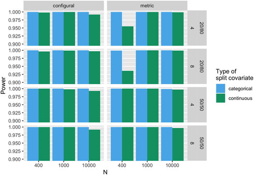
Figure 1 shows the power (i.e., the rate of correctly detecting a lack of MI; 1 - type II error rate) of EFA trees for all conditions. Overall, EFA trees demonstrated a high power of $>93\%$ for all conditions. EFA trees only missed a split in conditions where sample size was 400; for the conditions of sample size 1,000 and 10,000 the data was always split. However, in rare occasions for sample sizes 1,000 and 10,000, EFA trees chose the wrong covariate for splitting and then encountered problems of estimating the EFA models in the leaf nodes. We assume that this was due to too few observations in the nodes after a wrong split covariate (and thus, a wrong split point) was chosen. For the two conditions of sample size 400, ratio between groups 20/80, continuous split covariate, lack of metric MI, and number of distractors four and eight (ceteris paribus) the power was markedly smaller than for all other conditions (95.5% and 93.6%, respectively). Nonetheless, the power for these conditions can still be considered good and they are arguably the most complex conditions (small sample size, unbalanced groups, continuous covariate, and comparison of different sizes of cross-loadings).

Figure 1. Power (1 - type II error rate) of EFA trees to detect lack of measurement invariance (MI) by sample size N. Configural and metric denote the type of lack of MI. 20/80 and 50/50 denote the group size ratio. 4 and 8 denote the number of distractors.

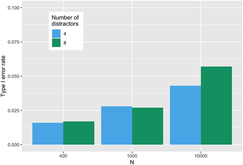
Figure 2 shows the type I error rates by sample size and by number of covariates. Most notably, the rate increased with sample size. The type I error rates did not markedly exceed the significance level we set for the EFA trees ($\alpha =0.05$). Only for a sample size of 10,000 and eight distractors the observed type I error rate was higher (0.057). When constructing an approximate 95% Wald-confidence interval (CI) around the observed type I error rates, the CI for sample size 10,000 contained the nominal level of significance $\alpha =0.05.$ However, for sample sizes 400 and 1,000 it did not contain 0.05. This could be an indication that the parameter stability tests are overly conservative. While from a statistical point of view this might not be ideal, the power to detect non-invariance was still high in our study. Nonetheless, future simulations should investigate the behavior of the type I error rate with even larger sample sizes or different test statistics.

Figure 2. Type I error rate (false-positive rate) of EFA trees by sample size N and number of distractors.

Table 10 shows the SRMRs for all conditions in the leaf nodes as well as the corresponding split rates (i.e., power and type I error rate). As can be seen, all SRMRs were $<0.03$ with $SD<0.01.$ Differences were most notable between sample sizes, such that SRMRs were smaller with increasing sample size. This seems reasonable as larger samples allow for more accurate model estimation.

Table 10. Mean and standard deviations of the standardized root mean squared residuals in the two leaf nodes and split rates for all 54 conditions.

Condition	Child Node 1	Child Node 2	SD1	SD2	Split Rate
1000, 4, 20/80, categorical, configural	0.016	0.012	0.0014	0.0014	1.000
1000, 4, 20/80, categorical, metric	0.015	0.010	0.0015	0.0012	1.000
1000, 4, 20/80, continuous, configural	0.012	0.016	0.0009	0.0018	1.000
1000, 4, 20/80, continuous, metric	0.010	0.016	0.0008	0.0018	1.000
1000, 4, 50/50, categorical, configural	0.010	0.015	0.0008	0.0013	1.000
1000, 4, 50/50, categorical, metric	0.010	0.013	0.0008	0.0012	1.000
1000, 4, 50/50, continuous, configural	0.015	0.010	0.0012	0.0024	0.998
1000, 4, 50/50, continuous, metric	0.013	0.010	0.0011	0.0026	1.000
1000, 4, none, none, none	0.007	0.010	0.0013	0.0031	0.028
1000, 8, 20/80, categorical, configural	0.016	0.012	0.0014	0.0013	1.000
1000, 8, 20/80, categorical, metric	0.015	0.010	0.0014	0.0008	1.000
1000, 8, 20/80, continuous, configural	0.012	0.016	0.0009	0.0017	0.999
1000, 8, 20/80, continuous, metric	0.010	0.015	0.0008	0.0016	1.000
1000, 8, 50/50, categorical, configural	0.010	0.015	0.0008	0.0012	1.000
1000, 8, 50/50, categorical, metric	0.010	0.013	0.0008	0.0014	1.000
1000, 8, 50/50, continuous, configural	0.015	0.010	0.0012	0.0021	1.000
1000, 8, 50/50, continuous, metric	0.013	0.010	0.0010	0.0022	1.000
1000, 8, none, none, none	0.007	0.012	0.0010	0.0053	0.027
10000, 4, 20/80, categorical, configural	0.005	0.004	0.0004	0.0009	1.000
10000, 4, 20/80, categorical, metric	0.005	0.003	0.0004	0.0007	1.000
10000, 4, 20/80, continuous, configural	0.004	0.005	0.0003	0.0018	0.992
10000, 4, 20/80, continuous, metric	0.003	0.005	0.0002	0.0005	0.999
10000, 4, 50/50, categorical, configural	0.003	0.005	0.0002	0.0005	1.000
10000, 4, 50/50, categorical, metric	0.003	0.004	0.0002	0.0006	0.999
10000, 4, 50/50, continuous, configural	0.005	0.003	0.0003	0.0009	0.993
10000, 4, 50/50, continuous, metric	0.004	0.003	0.0003	0.0007	0.997
10000, 4, none, none, none	0.002	0.003	0.0004	0.0008	0.043
10000, 8, 20/80, categorical, configural	0.005	0.004	0.0004	0.0011	1.000
10000, 8, 20/80, categorical, metric	0.005	0.003	0.0004	0.0009	1.000
10000, 8, 20/80, continuous, configural	0.004	0.005	0.0003	0.0005	0.997
10000, 8, 20/80, continuous, metric	0.003	0.005	0.0002	0.0005	0.999
10000, 8, 50/50, categorical, configural	0.003	0.005	0.0002	0.0006	1.000
10000, 8, 50/50, categorical, metric	0.003	0.004	0.0002	0.0004	1.000
10000, 8, 50/50, continuous, configural	0.005	0.003	0.0003	0.0011	0.992
10000, 8, 50/50, continuous, metric	0.004	0.003	0.0003	0.0011	0.997
10000, 8, none, none, none	0.002	0.003	0.0004	0.0008	0.057
400, 4, 20/80, categorical, configural	0.025	0.019	0.0028	0.0014	1.000
400, 4, 20/80, categorical, metric	0.025	0.016	0.0027	0.0013	1.000
400, 4, 20/80, continuous, configural	0.019	0.026	0.0015	0.0032	0.998
400, 4, 20/80, continuous, metric	0.016	0.025	0.0014	0.0032	0.955
400, 4, 50/50, categorical, configural	0.015	0.024	0.0014	0.0020	1.000
400, 4, 50/50, categorical, metric	0.015	0.021	0.0015	0.0018	1.000
400, 4, 50/50, continuous, configural	0.024	0.016	0.0020	0.0021	1.000
400, 4, 50/50, continuous, metric	0.021	0.016	0.0019	0.0019	1.000
400, 4, none, none, none	0.011	0.017	0.0014	0.0065	0.016
400, 8, 20/80, categorical, configural	0.025	0.019	0.0030	0.0014	1.000
400, 8, 20/80, categorical, metric	0.026	0.016	0.0027	0.0014	0.999
400, 8, 20/80, continuous, configural	0.019	0.025	0.0015	0.0031	0.996
400, 8, 20/80, continuous, metric	0.016	0.025	0.0015	0.0031	0.936
400, 8, 50/50, categorical, configural	0.016	0.024	0.0014	0.0019	1.000
400, 8, 50/50, categorical, metric	0.015	0.021	0.0014	0.0018	1.000
400, 8, 50/50, continuous, configural	0.024	0.016	0.0020	0.0020	1.000
400, 8, 50/50, continuous, metric	0.021	0.015	0.0019	0.0021	1.000
400, 8, none, none, none	0.011	0.016	0.0014	0.0040	0.017

Note. SD: standard deviation. Condition: First entry corresponds to sample size, second to number of distractors, third to group size ratio, fourth to type of split covariate, fifth to type of lack of measurement invariance.

8. Discussion

We investigated EFA trees as a method to explore and test for MI in a sample of questionnaire data. Our toy examples showed that EFA trees can be used as a simple and straightforward extension of methods that substantive researchers are familiar with. The comprehensive simulation study further highlighted that EFA trees perform well under various conditions. In all conditions, EFA trees demonstrated a high power to detect non-invariance while keeping false-positive splits in the pre-specified range. Ultimately, our goal is to suggest a method that helps researchers to develop questionnaires that took MI into account from the beginning. Additionally, EFA trees can be used as a first tool of exploration when analyzing data before more rigorous steps to test for MI are employed. This is particularly useful when there are no hypotheses about covariates that might cause non-invariance. Even for questionnaires developed as invariant as possible, these tests for MI prior to analyses are indispensable. One should keep in mind here that MI cannot be considered a characteristic of a construct but needs to be addressed for every construct in every study (Vandenberg, 2002).

8.1. Why Should You Use EFA Trees?

From a conceptually and theoretically broader perspective, we see three main advantages of EFA trees (and the same applies, in our opinion, to SEM trees and Rasch trees). First, both the seminal review by Vandenberg and Lance (2000) and the more recent one by Putnick and Bornstein (2016) showed that there is a high interest and need for tools that can explore and test for MI. This is good news because addressing MI related issues helps to improve the quality of psychological measurement. In all areas of psychology, improving measurement quality should be a main goal. Otherwise, ever more sophisticated data analysis methods (most notably, machine learning algorithms) cannot unfold their full potential. In fact, as Jacobucci and Grimm (2020) demonstrated, only small amounts of measurement error already diminish the effectiveness of machine learning algorithms to model non-linear effects. Of course, these tree-based methods will not solve all measurement bias related problems. But by equipping researchers with easy-to-use methods whose outputs they are used to interpreting, we can hopefully reduce measurement bias induced by non-invariance or DIF.

Second, EFA trees can assist researchers in shortening questionnaires or in item selection by enabling data-driven exploration of your sample. In practice, one of the main drivers when selecting “good” from “bad” items is the magnitude of factor loadings (Kleka & Soroko, 2018). However, this neglects the fact that even items with a small loading might be important from a content validity standpoint. Even further, there are various reasons why a lack of MI might occur that are arguably more important than loadings when deciding whether to keep or drop/exchange an item. Chen (2008) states many reasons, for example: a) the conceptual meaning or understanding of the construct differs across groups (e.g., for cultural reasons), b) particular items are more applicable for one group than another, c) the item was not translated properly, and/or d) certain groups respond to extreme items differently. EFA trees do not tell you directly which of these reasons applies to your situation. But they still identify items or whole scales that can then be further explored⁴. In the broadest sense, this might even inform psychological theory development if items are repeatedly shown to be non-invariant between certain groups (Brandmaier & Jacobucci, 2023). Put simply, an item with a small loading might be preferable to an item that works differently between groups (given that the small loading is not due to non-invariance caused by a covariate that was unmeasured and, thus, undetected by an EFA tree).

Third, EFA trees might help to improve the quality of decisions in single-case assessment. In general research, a lack of MI might lead to meaningless results of comparisons between groups. However, in diagnostic decision making on the single-case level, a lack of MI might cause misclassifications. It is common to incorporate diagnostic evidence gathered by tests like personality questionnaires or symptom severity scales when assessing whether a person is suitable for a job or eligible for a certain treatment. Ultimately, besides researching human behavior, this is the main reason why psychological tests are developed in the first place. Thus, it is crucial to develop questionnaires that are as invariant as possible between all potential target groups (Borsboom, 2006). Of course, this is an overly optimistic goal but we should then at least know for which groups a questionnaire can be used. Imagine using a depression scale that works differently for men and women, such that men receive lower test scores of depressivity even though their true score is equal to that of women. As a consequence, men would on average receive less diagnoses and, thus, less treatment for their depression or women would be overdiagnosed and overtreated in return. Therefore, easy-to-use methods for the assessment of MI on a high level can be a powerful tool to create fair and broadly applicable measures.

8.2. How Deep is Your Tree?

One important question we have not yet addressed directly is the depth of EFA trees. We have mostly talked about EFA trees that split the data once but have also shown that deeper trees are possible, revealing interactions between covariates. Theoretically, there is no limit on the depth of a tree (e.g., see Brandmaier et al., 2013b for SEM trees with up to four splits). However, we recommend that you decide on the depth of your tree depending on the goal of your analysis (if multiple interactions between covariates that are associated with non-invariance are present). The main areas of application of EFA trees are the earliest stages of questionnaire development and prior to specific analyses between two groups. In both scenarios, we see two main points to consider when deciding on the depth of your tree: sample size and interpretability.

First, sample sizes in the nodes have to be sufficiently large to allow for stable model estimations. Only then meaningful conclusions about the structure can be drawn. When we consider classic recommendations (Fabrigar et al., 1999) and current practice (Goretzko et al., 2021) regarding sample sizes in EFA, splitting more than once or twice might lead to too few observations in the leaf nodes.

Second, the heterogeneous groups identified by EFA trees should be reasonably interpretable (cf. Zeileis et al., 2008). As mentioned earlier, a split is always dependent on all prior splits. Especially in the earliest stages of questionnaire development, a main goal should be to identify non-invariant groups on a high level. Additionally, as explained in the Introduction, EFA trees use hierarchical clustering. That is, each split is conditional on the previous split. While this allows to determine the number of heterogeneous groups in a data-driven manner, the allocation of observations to the leaf nodes might not be optimal from a clustering perspective. This is less of a problem with shallow trees, whereas it is amplified when trees become deeper because more interactions are present. Thus, the deeper the tree is grown, we would recommend to be more cautious not to overinterpret the models in the leaf nodes.

8.3. Limitations and Future Directions

Inevitably, EFA trees come with a few limitations that researchers should keep in mind when applying the method. One issue when working with a single tree-based algorithm is that it is dependent on the specific sample (Breiman, 2001). To counteract this dependency, ensemble learning methods like random forests can be applied. In a random forest, multiple decision trees are grown in parallel and the results of all trees are aggregated into a single, more stable prediction of unseen data. Brandmaier et al. (2016) suggest SEM forests as an extension to SEM trees. They argue that SEM forests should not be seen as a “better” version of SEM trees but that both algorithms are complementary analyses. While SEM trees captivate by their interpretability and the information they yield about a sample at hand, specific partitions may not be optimal or may not generalize to new samples. SEM forests, in turn, can be used to obtain more stable estimates about covariates that predict difference in data patterns. Analogously, EFA trees can be extended to EFA forests. We want to point out two cautionary notes regarding this extension. First, it should be noted that growing even a single tree can be very expensive from a computational point of view. If a continuous covariate is identified as a split variable, the exhaustive search of order $O(N)$ can take well over one hour to yield a split point (on a standard local machine). Considering typical ensemble sizes of random forest (say 500 single trees), this can be time consuming even with parallelization on two or four cores. Of course, researchers who have supercomputing clusters available can make use of more cores for larger parallelization setups. Second, while the dependence on a specific sample makes decision trees unstable in their predictions of new data, the assessment of MI with respect to the present sample is the primary goal of EFA trees. The main strength of EFA trees lays in interpretability which we regard higher than predictive performance in this context (cf. Zeileis et al., 2008). Although an ensemble approach like random forests increases the generalizability of predictions, it impedes the inspection of a specific partition. If the goal is to obtain an interpretable structure for a sample at hand, a single EFA tree should be preferred.

As mentioned earlier, EFA models in the tree are estimated using maximum likelihood estimation (MLE). Unfortunately, so far no other estimation method can be applied because the hypothesis tests used to test for parameter differences need a well-defined likelihood (Hothorn et al., 2006; Zeileis et al., 2008; Zeileis & Hornik, 2007). Even though MLE is one of the most commonly used estimation methods for EFA, it is only suitable for multivariate normal data (Fabrigar et al., 1999; Goretzko et al., 2021). With the typical use of Likert-type items in psychological questionnaires (especially when answer options are few), this assumption of normality is questionable. Researchers should evaluate whether MLE is suitable for their data before applying EFA trees. Additionally, future studies are needed to assess the performance of EFA trees under non-normal data, for example with a dichotomous item format.

Another limitation one should keep in mind is that the sensitivity of the tree can only be governed by the level of significance that is set for the hypothesis tests rather than by considering effect sizes. That is, EFA trees are calibrated in a frequentist manner without really taking into account the impact of non-invariance on the subsequent analyses. Measures exist that directly link the degree of non-invariance to the impact it has on substantive analyses between groups (e.g., EPC-interest, Oberski, 2014). Moreover, Chen (2007) comprehensively evaluated the sensitivity of common goodness-of-fit indexes like SRMR to lack of MI. However, when using EFA trees, one can calibrate the trees only abstractly by adjusting the level of significance. That is, the higher the level of significance, the higher the sensitivity to detect smaller degrees of non-invariance. Similarly, if sample sizes become larger, smaller degrees of non-invariance become statistically significant without being practically relevant. It is crucial to thoroughly investigate the models in the leaf nodes to identify whether a split is actually meaningful. Here, too, can domain expertise help to identify possible false-positive splits. Future research should investigate measures that could govern the sensitivity of the tree by considering minimum non-invariance thresholds (i.e., a minimum degree of non-invariance that is deemed relevant for splitting).

The last limitation was raised by Strobl et al. (2015) in the context of Rasch trees and equally applies to EFA trees: If a covariate that causes non-invariance has not been measured, it cannot be detected by the tree. However, if a covariate that is correlated with the relevant missing one is available, non-invariance may still be detected (Strobl et al., 2015). For this reason, a covariate identified for splitting the data cannot simply be interpreted as the root cause of the lack of MI. That is, any split covariate might well be just the observed version of a latent variable causing non-invariance. This again highlights the importance of thoroughly investigating the data and to use EFA trees as a means of exploration.

9. Conclusion

EFA trees offer an easy-to-use and well-known approach to exploring data and testing for MI. They are especially useful in areas like personality or clinical psychology where constructs can be multidimensional and complex. We hope to motivate researchers to test for MI in the earliest stages of questionnaire development but also before substantive group comparisons. In this, measurement bias in general research will hopefully be reduced and diagnostic decisions might even become fairer. When it comes down to it, there is hardly any area of psychology or any research question that would not benefit from more measurement invariance. Or, to put it in the words of Meredith (1993) (p. 540): “It should be obvious that measurement invariance […] are idealizations. They are, however, enormously useful idealizations in their application to psychological theory building and evaluation.”

Acknowledgements

The authors thank Florian Pargent and Rudolf Debelak for valuable comments on our manuscript. Parts of the current article were presented by the first author at the 2022 Conference of the Psychometric Society in Bologna, Italy and at the 2022 Conference of the German Psychological Society in Hildesheim, Germany. A preprint of the article was published on PsyArXiv. The analyses scripts and supplementary material supporting this article are openly available on the Open Science Framework on https://osf.io/7pgrb/. The authors made the following contributions. Philipp Sterner: Conceptualization, Formal Analysis, Methodology, Visualization, Writing - Original Draft; David Goretzko: Conceptualization, Methodology, Writing - Review & Editing, Supervision.

Notes

1 To be able to test hypotheses about obliquely rotated factor loadings, Jennrich (1973) showed how to derive the required standard errors.

2 An interesting extension could be to combine EFA trees with the aforementioned multigroup factor rotation (MGFR; De Roover & Vermunt, 2019). Instead of regularizing the models in the nodes, MGFR could be applied to investigate group-specific measurement models in the leaf nodes. One advantage of this approach over regularization would be that one could pinpoint the parameters that differ across the nodes.

3 During the review process, one reviewer posed the question whether EFA trees would also split the data if differences occured only in factor correlations between groups. We have created an online supplement in which we show that EFA trees split the data in this case and demonstrate what this entails for the invariance of measurements. Additionally, we discuss the use of covariance instead of correlation matrices when estimating the models in the leaf nodes. The online supplement is openly available at https://osf.io/7pgrb/.

4 Note that if factor solutions in the nodes are rotated instead of regularized, the items or scales that are identified as non-invariant depend on the exact factor rotation. This is because the solutions are no longer unique and thus different rotations might lead to different interpretations of the solutions. Regularized solutions are unique given a specific type of regularization (e.g., LASSO, ridge, or elastic net) and a specific set of hyperparameters. Changing these settings might again yield different interpretations.

References

- Ammerman, B. A., Jacobucci, R., & McCloskey, M. S. (2019). Reconsidering important outcomes of the nonsuicidal self-injury disorder diagnostic criterion A. Journal of Clinical Psychology, 75, 1084–1097. https://doi.org/10.1002/jclp.22754
- Asparouhov, T., & Muthén, B. O. (2009). Exploratory Structural Equation Modeling. Structural Equation Modeling: A Multidisciplinary Journal, 16, 397–438. https://doi.org/10.1080/10705510903008204
- Asparouhov, T., & Muthén, B. O. (2014). Multiple-group factor analysis alignment. Structural Equation Modeling: A Multidisciplinary Journal, 21, 495–508. https://doi.org/10.1080/10705511.2014.919210
- Aust, F., & Barth, M. (2020). Papaja: Create APA manuscripts with R Markdown.
- Borsboom, D. (2006). When does measurement invariance matter? Medical Care, 44, 176–181. https://doi.org/10.1097/01.mlr.0000245143.08679.cc
- Brandmaier, A. M., Driver, C. C., & Voelkle, M. C. (2018). Recursive partitioning in continuous time analysis. In K. van Montfort, J. H. L. Oud, & M. C. Voelkle (Eds.), Continuous time modeling in the behavioral and related sciences (pp. 259–282). Springer.
- Brandmaier, A. M., & Jacobucci, R. (2023). Machine-learning approaches to structural equation modeling. In R. A. Hoyle (Ed.), Handbook of structural equation modeling (pp. 722–739). Guilford Press.
- Brandmaier, A. M., Prindle, J. J., McArdle, J. J., & Lindenberger, U. (2016). Theory-guided exploration with structural equation model forests. Psychological Methods, 21, 566–582. https://doi.org/10.1037/met0000090
- Brandmaier, A. M., Ram, N., Wagner, G. G., & Gerstorf, D. (2017). Terminal decline in well-being: The role of multi-indicator constellations of physical health and psychosocial correlates. Developmental Psychology, 53, 996–1012. https://doi.org/10.1037/dev0000274
- Brandmaier, A. M., von Oertzen, T., McArdle, J. J., & Lindenberger, U. (2013a). Exploratory data mining with structural equation model trees. In J. J. McArdle & G. Ritschard (Eds.), Contemporary Issues in Exploratory Data Mining in the Behavioral Sciences (pp. 96–127). Routledge.
- Brandmaier, A. M., von Oertzen, T., McArdle, J. J., & Lindenberger, U. (2013b). Structural equation model trees. Psychological Methods, 18, 71–86. https://doi.org/10.1037/a0030001
- Breiman, L. (2001). Random forests. Machine Learning, 45, 5–32. https://doi.org/10.1023/A:1010933404324
- Browne, M. W. (2001). An overview of analytic rotation in exploratory factor analysis. Multivariate Behavioral Research, 36, 111–150. https://doi.org/10.1207/S15327906MBR3601_05
- Chen, F. F. (2007). Sensitivity of goodness of fit indexes to lack of measurement invariance. Structural Equation Modeling: A Multidisciplinary Journal, 14, 464–504. https://doi.org/10.1080/10705510701301834
- Chen, F. F. (2008). What happens if we compare chopsticks with forks? The impact of making inappropriate comparisons in cross-cultural research. Journal of Personality and Social Psychology, 95, 1005–1018. https://doi.org/10.1037/a0013193
- de Mooij, S. M., Henson, R. N., Waldorp, L. J., & Kievit, R. A. (2018). Age differentiation within gray matter, white matter, and between memory and white matter in an adult life span cohort. The Journal of Neuroscience : The Official Journal of the Society for Neuroscience, 38, 5826–5836. https://doi.org/10.1523/JNEUROSCI.1627-17.2018
- De Roover, K. (2021). Finding clusters of groups with measurement invariance: Unraveling intercept non-invariance with mixture multigroup factor analysis. Structural Equation Modeling: A Multidisciplinary Journal, 28, 663–683. https://doi.org/10.1080/10705511.2020.1866577
- De Roover, K., & Vermunt, J. K. (2019). On the exploratory road to unraveling factor loading non-invariance: A new multigroup rotation approach. Structural Equation Modeling: A Multidisciplinary Journal, 26, 905–923. https://doi.org/10.1080/10705511.2019.1590778
- De Roover, K., Vermunt, J. K., & Ceulemans, E. (2022). Mixture multigroup factor analysis for unraveling factor loading noninvariance across many groups. Psychological Methods, 27, 281–306. https://doi.org/10.1037/met0000355
- Debelak, R., & Strobl, C. (2019). Investigating measurement invariance by means of parameter instability tests for 2PL and 3PL models. Educational and Psychological Measurement, 79, 385–398. https://doi.org/10.1177/0013164418777784
- Dolan, C. V., Oort, F. J., Stoel, R. D., & Wicherts, J. M. (2009). Testing measurement invariance in the target rotated multigroup exploratory factor model. Structural Equation Modeling: A Multidisciplinary Journal, 16, 295–314. https://doi.org/10.1080/10705510902751416
- Fabrigar, L. R., Wegener, D. T., MacCallum, R. C., & Strahan, E. J. (1999). Evaluating the use of exploratory factor analysis in psychological research. Psychological Methods, 4, 272–299. https://doi.org/10.1037/1082-989X.4.3.272
- Genz, A., Bretz, F., Miwa, T., Mi, X., Leisch, F., Scheipl, F., … Hothorn, M. T. (2002). Package ‘mvtnorm. Journal of Computational and Graphical Statistics, 11, 950–971. https://doi.org/10.1198/106186002394
- Goretzko, D., & Bühner, M. (2022). Note: Machine learning modeling and optimization techniques in psychological assessment. Psychological Test and Assessment Modeling, 64, 3–21.
- Goretzko, D., Pham, T. T. H., & Bühner, M. (2021). Exploratory factor analysis: Current use, methodological developments and recommendations for good practice. Current Psychology, 40, 3510–3521. https://doi.org/10.1007/s12144-019-00300-2
- Hirose, K., & Yamamoto, M. (2014). Estimation of an oblique structure via penalized likelihood factor analysis. Computational Statistics & Data Analysis, 79, 120–132. https://doi.org/10.1016/j.csda.2014.05.011
- Holland, P. W., & Wainer, H. (2012). Differential item functioning. Routledge.
- Horn, J. L. (1965). A rationale and test for the number of factors in factor analysis. Psychometrika, 30, 179–185. https://doi.org/10.1007/BF02289447
- Hothorn, T., Hornik, K., & Zeileis, A. (2006). Unbiased recursive partitioning: A conditional inference framework. Journal of Computational and Graphical Statistics, 15, 651–674. https://doi.org/10.1198/106186006X133933
- Hothorn, T., & Zeileis, A. (2015). Partykit: A modular toolkit for recursive partytioning in R. The Journal of Machine Learning Research, 16, 3905–3909.
- Jacobucci, R., & Grimm, K. J. (2020). Machine learning and psychological research: The unexplored effect of measurement. Perspectives on Psychological Science : a Journal of the Association for Psychological Science, 15, 809–816. https://doi.org/10.1177/1745691620902467
- Jacobucci, R., Grimm, K. J., Brandmaier, A. M., Serang, S., Kievit, R. A., Scharf, F., … Jacobucci, M. R. (2016). Package ‘regsem.’
- Jacobucci, R., Grimm, K. J., & McArdle, J. J. (2016). Regularized structural equation modeling. Structural Equation Modeling : a Multidisciplinary Journal, 23, 555–566. https://doi.org/10.1080/10705511.2016.1154793
- Jacobucci, R., Grimm, K. J., & McArdle, J. J. (2017). A comparison of methods for uncovering sample heterogeneity: Structural equation model trees and finite mixture models. Structural Equation Modeling : a Multidisciplinary Journal, 24, 270–282. https://doi.org/10.1080/10705511.2016.1250637
- Jennrich, R. I. (1973). Standard errors for obliquely rotated factor loadings. Psychometrika, 38, 593–604. https://doi.org/10.1007/BF02291497
- Jöreskog, K. G. (1967). Some contributions to maximum likelihood factor analysis. Psychometrika, 32, 443–482. https://doi.org/10.1007/BF02289658
- Kiers, H. A. L. (1994). Simplimax: Oblique rotation to an optimal target with simple structure. Psychometrika, 59, 567–579. https://doi.org/10.1007/BF02294392
- Kim, E. S., Cao, C., Wang, Y., & Nguyen, D. T. (2017). Measurement invariance testing with many groups: A comparison of five approaches. Structural Equation Modeling: A Multidisciplinary Journal, 24, 524–544. https://doi.org/10.1080/10705511.2017.1304822
- Kleka, P., & Soroko, E. (2018). How to avoid the sins of questionnaires abridgement? Survey Research Methods, 12, 147–160. https://doi.org/10.18148/srm/2018.v12i2.7224
- Komboz, B., Strobl, C., & Zeileis, A. (2018). Tree-based global model tests for polytomous Rasch models. Educational and Psychological Measurement, 78, 128–166. https://doi.org/10.1177/0013164416664394
- Li, X., Jacobucci, R., & Ammerman, B. A. (2021). Tutorial on the Use of the regsem Package in R. Psych, 3, 579–592. https://doi.org/10.3390/psych3040038
- Meade, A. W., & Lautenschlager, G. J. (2004). A comparison of item response theory and confirmatory factor analytic methodologies for establishing measurement equivalence/invariance. Organizational Research Methods, 7, 361–388. https://doi.org/10.1177/1094428104268027
- Meredith, W. (1993). Measurement invariance, factor analysis and factorial invariance. Psychometrika, 58, 525–543. https://doi.org/10.1007/BF02294825
- Merkle, E. C., Fan, J., & Zeileis, A. (2014). Testing for measurement invariance with respect to an ordinal variable. Psychometrika, 79, 569–584. https://doi.org/10.1007/s11336-013-9376-7
- Merkle, E. C., & Zeileis, A. (2013). Tests of measurement invariance without subgroups: A generalization of classical methods. Psychometrika, 78, 59–82. https://doi.org/10.1007/s11336-012-9302-4
- Milfont, T. L., & Fischer, R. (2010). Testing measurement invariance across groups: Applications in cross-cultural research. International Journal of Psychological Research, 3, 111–130. https://doi.org/10.21500/20112084.857
- Millsap, R. E. (2012). Statistical approaches to measurement invariance. Routledge.
- Mulaik, S. A. (2010). Foundations of factor analysis. CRC press.
- Muthén, B. O. (1989). Latent variable modeling in heterogeneous populations. Psychometrika, 54, 557–585. https://doi.org/10.1007/BF02296397
- Oberski, D. L. (2014). Evaluating sensitivity of parameters of interest to measurement invariance in latent variable models. Political Analysis, 22, 45–60. https://doi.org/10.1093/pan/mpt014
- Putnick, D. L., & Bornstein, M. H. (2016). Measurement invariance conventions and reporting: The state of the art and future directions for psychological research. Developmental Review : DR, 41, 71–90. https://doi.org/10.1016/j.dr.2016.06.004
- R Core Team. (2021). R: A Language and Environment for Statistical Computing. R Foundation for Statistical Computing.
- Rosseel, Y. (2012). Lavaan: An R package for structural equation modeling. Journal of Statistical Software, 48, 1–36. https://doi.org/10.18637/jss.v048.i02
- Rutkowski, L., & Svetina, D. (2014). Assessing the hypothesis of measurement invariance in the context of large-scale international surveys. Educational and Psychological Measurement, 74, 31–57. https://doi.org/10.1177/0013164413498257
- Sass, D. A. (2011). Testing measurement invariance and comparing latent factor means within a confirmatory factor analysis framework. Journal of Psychoeducational Assessment, 29, 347–363. https://doi.org/10.1177/0734282911406661
- Sass, D. A., & Schmitt, T. A. (2010). A comparative investigation of rotation criteria within exploratory factor analysis. Multivariate Behavioral Research, 45, 73–103. https://doi.org/10.1080/00273170903504810
- Scharf, F., & Nestler, S. (2019). Should regularization replace simple structure rotation in exploratory factor analysis? Structural Equation Modeling: A Multidisciplinary Journal, 26, 576–590. https://doi.org/10.1080/10705511.2018.1558060
- Schneider, L., Strobl, C., Zeileis, A., & Debelak, R. (2021). An R toolbox for score-based measurement invariance tests in IRT models. Behavior Research Methods, 54, 2101–2113. https://doi.org/10.3758/s13428-021-01689-0
- Simpson-Kent, I. L., Fuhrmann, D., Bathelt, J., Achterberg, J., Borgeest, G. S., & Kievit, R. A, CALM Team. (2020). Neurocognitive reorganization between crystallized intelligence, fluid intelligence and white matter microstructure in two age-heterogeneous developmental cohorts. Developmental Cognitive Neuroscience, 41, 100743. https://doi.org/10.1016/j.dcn.2019.100743
- Strobl, C., Kopf, J., & Zeileis, A. (2015). Rasch trees: A new method for detecting differential item functioning in the Rasch model. Psychometrika, 80, 289–316. https://doi.org/10.1007/s11336-013-9388-3
- Trendafilov, N. T. (2014). From simple structure to sparse components: A review. Computational Statistics, 29, 431–454. https://doi.org/10.1007/s00180-013-0434-5
- Usami, S., Hayes, T., & McArdle, J. (2017). Fitting structural equation model trees and latent growth curve mixture models in longitudinal designs: The influence of model misspecification. Structural Equation Modeling: A Multidisciplinary Journal, 24, 585–598. https://doi.org/10.1080/10705511.2016.1266267
- Usami, S., Jacobucci, R., & Hayes, T. (2019). The performance of latent growth curve model-based structural equation model trees to uncover population heterogeneity in growth trajectories. Computational Statistics, 34, 1–22. https://doi.org/10.1007/s00180-018-0815-x
- Van de Schoot, R., Lugtig, P., & Hox, J. (2012). A checklist for testing measurement invariance. European Journal of Developmental Psychology, 9, 486–492. https://doi.org/10.1080/17405629.2012.686740
- Vandenberg, R. J. (2002). Toward a further understanding of and improvement in measurement invariance methods and procedures. Organizational Research Methods, 5, 139–158. https://doi.org/10.1177/1094428102005002001
- Vandenberg, R. J., & Lance, C. E. (2000). A review and synthesis of the measurement invariance literature: Suggestions, practices, and recommendations for organizational research. Organizational Research Methods, 3, 4–70. https://doi.org/10.1177/109442810031002
- Zeileis, A., & Hornik, K. (2007). Generalized M-fluctuation tests for parameter instability. Statistica Neerlandica, 61, 488–508. https://doi.org/10.1111/j.1467-9574.2007.00371.x
- Zeileis, A., Hothorn, T., & Hornik, K. (2008). Model-based recursive partitioning. Journal of Computational and Graphical Statistics, 17, 492–514. https://doi.org/10.1198/106186008X319331
- Zou, H., & Hastie, T. (2005). Regularization and variable selection via the elastic net. Journal of the Royal Statistical Society: Series B, 67, 301–320. https://doi.org/10.1111/j.1467-9868.2005.00503.x