Striving for Sparsity: On Exact and Approximate Solutions in Regularized Structural Equation Models

Abstract

Regularized structural equation models have gained considerable traction in the social sciences. They promise to reduce overfitting by focusing on out-of-sample predictions and sparsity. To this end, a set of increasingly constrained models is fitted to the data. Subsequently, one of the models is selected, usually by means of information criteria. Current implementations of regularized structural equation models differ in their optimizers: Some use general purpose optimizers whereas others use specialized optimization routines. While both approaches often perform similarly, we show that they can produce very different results. We argue that in particular, the interaction between optimizer and selection criterion (e.g., BIC) contributes to these differences. We substantiate our arguments with an empirical demonstration and a simulation study. Based on these findings, we conclude that researchers should consider specialized optimizers whenever possible. To facilitate the implementation of such optimizers, we provide the R package lessSEM.

Keywords:

• Lasso
• optimization
• regularization
• structural equation model

Structural equation modeling (SEM) is a confirmatory framework, where a model is first specified and then fitted to the data set. To this end, knowledge about each and every effect, (co-)variance, and intercept included in the model is required (e.g., based on theoretical considerations and prior analyses). Often, however, little is known about the underlying mechanisms and structure of the psychological constructs under investigation. Even in well-established fields, purely confirmatory modeling can fail to adequately reflect the data due to the rigidity of the underlying framework (e.g., Marsh et al., 2010).

Regularized SEM has been proposed as a compromise between the confirmatory SEM and exploratory model search strategies (Huang et al., 2017; Jacobucci et al., 2016). This “semi-confirmatory approach” (Huang et al., 2017, p. 330) allows for more flexibility during data analysis, while still operating in a framework familiar to many social scientists. Regularized SEM has a strong focus on the predictive performance and sparsity of the model (Huang et al., 2017; Jacobucci et al., 2016). To this end, selected parameter estimates are shrunken toward zero (Tibshirani, 1996). This shrinkage restricts the degree to which a model is allowed to adapt to the data set and can improve its predictive performance if applied carefully (e.g., Huang et al., 2017; Jacobucci et al., 2016; Tibshirani, 1996). Additionally, many regularization techniques can set parameter estimates to zero, resulting in sparser models which may simplify the interpretation considerably (e.g., Fan & Li, 2001; Tibshirani, 1996; Zhang, 2010; Zou, 2006). The aforementioned properties make a compelling argument for the use of regularized SEM, which has consequently gained a foothold in the social sciences (e.g., Davis et al., 2019; Epskamp et al., 2017; Finch & Miller, 2021; Friemelt et al., 2022; Góngora et al., 2020; Jacobucci et al., 2019; Jacobucci & Grimm, 2018; Koncz et al., 2022; Scharf & Nestler, 2019; Ye et al., 2021).

The R (R Core Team, 2022) packages regsem (Jacobucci, 2017) and lslx (Huang, 2020a) greatly simplify fitting regularized SEMs. While regsem and lslx differ in their features,¹ most “standard” SEMs can be regularized with both packages and—in theory—regsem and lslx should result in similar parameter estimates. Direct comparisons, however, suggest performance differences, for instance, in terms of the final fitting function value (Huang, 2020a), the number of non-convergent results (Finch & Miller, 2021; Friemelt et al., 2022; Huang, 2020a), and the predictive performance (Finch & Miller, 2021; Geminiani et al., 2021).

It is important to understand the roots of such differences, both theoretically (e.g., when implementing regularization methods for other models) and practically (e.g., when choosing between different implementations of the same methods). Huang (2018) attributes some differences to the optimizers used by both packages. While the default setting in regsem is to rely on a general purpose optimizer that is not adapted to the specific penalty functions, Huang (2020a) implemented specialized optimizers (regsem optionally provides a specialized optimizer as well). For lasso regularization, Huang (2018) states that the method by Jacobucci (2017) “cannot efficiently find a local maximizer, especially when the model is relatively complex” (Huang, 2018, p. 500). Likewise, Orzek and Voelkle (2023) observed differences between general purpose optimizers and specialized optimizers in lasso regularized continuous time SEM and therefore used specialized optimizers. In contrast, Ridler (2022) used the general purpose optimizer after observing differences between both types of optimizers implemented in regsem based on the recommendation provided in the package. Furthermore, Belzak and Bauer (2020) used general purpose optimizers to assess differential item functioning in item response theory models and found that their implementation performed similarly to specialized optimizers (see also Belzak, 2021). Finally, Battauz (2020) found that a general purpose optimizer resulted in a better fit than specialized optimizers in regularized nominal response models. It, therefore, remains unclear if the finding by Orzek and Voelkle (2023) generalizes to the “standard” regularized SEM, where general purpose optimizers are already routinely used—a question that we set out to answer in this work.

In the following, we will first provide an introduction to regularized SEM, focusing specifically on the issue of optimization. Building on Orzek and Voelkle (2023), we will demonstrate the consequences of using general purpose optimizers with an empirical example and provide new insights with a simulation study. Our results indicate that differences in the optimization procedures could partially explain the performance discrepancies observed between regsem and lslx in the literature (e.g., Finch & Miller, 2021; Friemelt et al., 2022; Geminiani et al., 2021; Huang, 2020a). We conclude that researchers using regularized SEM should prefer specialized optimizers where available. To facilitate the development of regularized SEM we provide the new R package lessSEM.

1. The Two Steps of Regularized Structural Equation Modeling

At its core, regularized SEM is a two-step procedure: In the first step, a set of increasingly sparse models is estimated. This is followed by the second step, where one of the models is selected (e.g., Huang et al., 2017; Jacobucci et al., 2016; Tibshirani, 1996). Building on an extensive background of research on regularization techniques in machine learning (e.g., Fan & Li, 2001; Tibshirani, 1996; Zhang, 2010; Zou, 2006), different strategies for both steps, estimating increasingly sparse models and selecting one of these models, have been proposed in the regularized SEM framework (e.g., Huang et al., 2017; Jacobucci et al., 2016; Li & Jacobucci, 2021).

1.1. Step One: Estimating Increasingly Sparse Models

In regularized SEM, a set of increasingly sparse models is estimated by slightly altering the fitting function. This function is minimized when estimating the parameters $\mathit{\theta }.$ We will restrict the discussion to the commonly used −2 log-likelihood fitting function $F_{\text{ML}}(\mathit{\theta }).$ Furthermore, we will assume that the likelihood itself is given by the multivariate normal density function, the default in most SEM applications. In regularized SEM, $F_{\text{ML}}(\mathit{\theta })$ is combined with a penalty term $p(\mathit{\theta })$ (Huang et al., 2017; Jacobucci et al., 2016): (1) $$F_{\text{reg},\lambda }(\mathit{\theta })=F_{\text{ML}}(\mathit{\theta })+\lambda Np(\mathit{\theta })$$(1)

Finding the parameter estimates ${\widehat{\mathit{\theta }}}_{\lambda }$, which minimize $F_{\text{reg},\lambda }(\mathit{\theta })$, requires balancing the two forces in the new fitting function. This can be thought of as a tug-of-war, where $F_{\text{ML}}(\mathit{\theta })$ ties to pull $\mathit{\theta }$ to the maximum likelihood estimates ${\widehat{\mathit{\theta }}}_{\text{ML}}$ and $p(\mathit{\theta })$ pulls selected parameters toward zero. The tuning parameter $\lambda \ge 0$ allows for shifting the balance between these two forces: If λ is close to zero, the maximum likelihood part $F_{\text{ML}}(\mathit{\theta })$ will dominate the fitting function and parameters will be close to ${\widehat{\mathit{\theta }}}_{\text{ML}}.$ In contrast, if λ is very large, the penalty term $p(\mathit{\theta })$ will take over the fitting function and parameters will be close to zero (this is demonstrated in Figure 1 for different penalty functions $p(\mathit{\theta })$). We can conceive of λ as the ratio of players per team in our tug-of-war game which allows us to give one team an advantage over the other. Finally, the penalty term in Equation (1)(1) $$F_{\text{reg},\lambda }(\mathit{\theta })=F_{\text{ML}}(\mathit{\theta })+\lambda Np(\mathit{\theta })$$(1) is multiplied with sample size N to stay consistent with current implementations of regularized SEM in regsem and lslx. Importantly, the parameter λ itself is not estimated alongside the other parameters in $\mathit{\theta }.$ Instead, researchers must define a set of λ values (e.g., $\lambda \in \{0,.01,\dots ,1\}$) and fit a separate model for each of them (e.g., Jacobucci et al., 2016). Thus, the number of λ values dictates how many models are estimated (see Huang et al., 2017; Jacobucci et al., 2016, for more details).

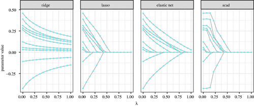
Many different penalty functions $p(\mathit{\theta })$ have been proposed, such as the ridge (Hoerl & Kennard, 1970), lasso (Tibshirani, 1996), adaptive lasso (Zou, 2006), elastic net (Zou & Hastie, 2005), scad (Fan & Li, 2001), lsp (Candès et al., 2008), cappedL1 (Zhang, 2010), and mcp (Zhang, 2010). Most importantly, the different penalty functions exhibit distinct properties. For instance, ridge regularization can only shrink parameters toward zero, while the other penalties mentioned above can shrink parameters and set them to zero; that is, they perform parameter selection (e.g., Tibshirani, 1996, see Figure 1 for a visualization of different penalty functions). In SEM this can, for instance, be used to identify non-zero cross-loadings (Scharf & Nestler, 2019) or to simplify multiple-indicator-multiple-causes models (Jacobucci et al., 2019). Most of the penalty functions mentioned above are implemented in the R packages regsem (Jacobucci, 2017) or lslx (Huang, 2020a). For simplicity, we will focus on lasso regularization in the following. However, we expect the results to be similar for all other penalties which use the absolute value function (e.g., adaptive lasso, elastic net, scad, lsp, cappedL1, and mcp). The lasso is defined as (2) $$p(\mathit{\theta })=\sum _{j=1}^J{r}_j\left|{\theta }_j\right|.$$(2)

Here, J is the number of parameters in $\mathit{\theta }$ and r_j is a selection operator. If r_j = 1, the parameter θ_j is regularized and if r_j = 0 the parameter θ_j remains unregularized. This allows for regularizing only a subset of the parameters, for instance, only the loadings. Finally, $|·|$ denotes the absolute value function.

1.2. Step Two: Selecting the Best Model

Different values of λ can result in vastly different parameter estimates (e.g., see Figure 1). This property was used in step one to estimate a set of increasingly sparse models. In step two, one of these models must be selected (i.e., an appropriate value for λ must be found). Too little regularization may result in an overly complex model that still overfits the data and generalizes poorly. Too much regularization, in contrast, may result in an overly sparse model that underfits the data. Different procedures for selecting λ have been proposed (e.g., Tibshirani, 1996). The most prominent in regularized SEM are cross-validation and information criteria (Huang et al., 2017; Jacobucci et al., 2016; Li et al., 2021).

Cross-validation provides a direct way to measure how well a model generalizes to data sets that come from the same population but have not been used to estimate the model parameters (e.g., Browne, 2000). To this end, the models are fitted on one part of the data set, using the remaining part to evaluate the out of sample fit. In k-fold cross-validation, the data set is split in k subsets. Subsequently, each subset serves as a test set while fitting the model using the left out k − 1 subsets (a general introduction to cross-validation is, for instance, provided by James et al., 2013). The main drawbacks of cross-validation are that (1) refitting the model on subsets of the data may result in non-convergence and worse parameter estimates due to the smaller sample size, and (2) depending on the complexity of the model, refitting the model may take a relatively long time. Therefore, cross-validated regularized SEM is rarely used in practice.

Information criteria are an alternative to cross-validation that do not require any refitting (asymptotically, information criteria and cross-validation are closely related; Shao, 1997; Stone, 1977). The Bayesian information criterion (BIC; Schwarz, 1978), for example, is defined as (3) $$\text{BIC}=F_{\text{ML}}(\mathit{\theta })+\hspace{0.17em}\log \hspace{0.17em}(N)t$$(3)

Smaller BIC values indicate better fit and can be achieved by either reducing $F_{\text{ML}}(\mathit{\theta })$ or by reducing the number of model parameters t. The latter can be seen as the BIC rewarding model sparsity. In regularized SEM, the BIC and similar information criteria are typically used to select the final parameters if the penalty can set them to zero and therefore reduce t (Huang et al., 2017; Jacobucci et al., 2016). Importantly, information criteria are currently the standard model selection procedure in regsem and lslx and are used in many recent publications (e.g., Brandmaier & Jacobucci, in press; Davis et al., 2019; Finch & Miller, 2021; Góngora et al., 2020; Huang et al., 2017; Jacobucci et al., 2019; Koncz et al., 2022; Li et al., 2021; Scharf & Nestler, 2019; Ye et al., 2021). However, as we will discuss in detail in the next section, combining information criteria with general purpose optimizers requires two additional parameters that determine which model gets selected (see also Orzek & Voelkle, 2023).

2. General Purpose and Specialized Optimizers

While adding the penalty function $p(\mathit{\theta })$ to $F_{\text{ML}}(\mathit{\theta })$ seems innocuous, it can have severe consequences for parameter estimation. Uncovering these consequences requires a closer look at optimization algorithms (see also Belzak, 2021; Orzek & Voelkle, 2023).

To estimate the model parameters ${\widehat{\mathit{\theta }}}_{\lambda },F_{\text{reg},\lambda }(\mathit{\theta })$ must be minimized. What sounds like a simple procedure is, in fact, a tedious process with numerous pitfalls. For the models under consideration here, there is (in general) no direct (i.e., closed form) solution to minimizing $F_{\text{reg},\lambda }(\mathit{\theta }).$ Instead, an iterative procedure is used which replaces the difficult to answer question “What is the minimum of $F_{\text{reg},\lambda }(\mathit{\theta })$?” with a simpler one: “Is there a parameter vector ${\mathit{\theta }}_{k+1}$ close to the current point ${\mathit{\theta }}_k$ that results in a smaller $F_{\text{reg},\lambda }(\mathit{\theta })$?” This question is asked repeatedly until no further improvement to ${\mathit{\theta }}_k$ can be made. Many different procedures that formalize and answer this surrogate question have been proposed, which differ in the functions they can minimize (see Nocedal & Wright, 2006, for an introduction). To better understand why $F_{\text{reg},\lambda }(\mathit{\theta })$ is a special problem, we will concentrate on so-called Newton-type optimization algorithms. Here, in each iteration k, one tries to take a step of length s_k in a downward direction ${\mathit{d}}_k.$ The new parameter vector ${\mathit{\theta }}_{k+1}$ is then given by: ${\mathit{\theta }}_{k+1}={\mathit{\theta }}_k+s_k{\mathit{d}}_k.$ A visual representation of this approach for a single parameter θ and fitting function $f(\theta )$ is provided in Figure 2. Note that we get closer to the minimum of the fitting function with each step.

Newton-type optimizers typically use the gradients and the Hessian of the fitting function to determine the step direction ${\mathit{d}}_k$ (e.g., Nocedal & Wright, 2006).² Therefore, they assume that both, the gradients and the Hessian, can be computed (this assumption is often stated as “$f:{\mathbb{R}}^n\to \mathbb{R}$ is a smooth function” or “$f:{\mathbb{R}}^n\to \mathbb{R}$ is continuously differentiable”; Nocedal & Wright, 2006, p. 10 and p. 14)

For $F_{\text{reg},\lambda }(\mathit{\theta })$ this leaves us with a problem: Whereas gradients and the Hessian for $F_{\text{ML}}(\mathit{\theta })$ are typically well defined (e.g., von Oertzen & Brick, 2013), this is not the case for any of the penalty functions introduced above, with the exception of ridge, which does not set parameters to zero. Figure 3 exemplarily shows the ridge and lasso penalty values for a single parameter. Note that the ridge penalty is smooth (or differentiable) whereas the lasso is non-smooth (or non-differentiable) at θ = 0. To demonstrate the non-differentiability of the lasso mathematically, we can rewrite the absolute value as $\left|{\theta }_j\right|=\sqrt{{\theta }_j^2},$ where $\sqrt{·}$ is the positive square root. Differentiating with respect to θ_j, we get: $\frac{\partial }{\partial {\theta }_j}\sqrt{{\theta }_j^2}=\frac{{\theta }_j}{\sqrt{{\theta }_j^2}}.$ If follows that $\frac{{\theta }_j}{\sqrt{{\theta }_j^2}}=1$ if ${\theta }_j>0,\frac{{\theta }_j}{\sqrt{{\theta }_j^2}}=-1$ if ${\theta }_j<0,$ and $\frac{{\theta }_j}{\sqrt{{\theta }_j^2}}$ results in division by zero if ${\theta }_j=0.$

The non-differentiability is essential for the parameter selection property of the lasso and related regularization procedures (e.g., Fan & Li, 2001): The steepness of the curves shown in Figure 3 corresponds to the force with which they push parameters to zero (Andrew & Gao, 2007). For the ridge penalty, the steepness decreases as θ approaches zero. As a consequence, any small force pushing θ away from zero ($F_{\text{ML}}(\mathit{\theta })$ in our case) will overrule the ridge penalty and parameters will stay non-zero. Contrast this with the lasso penalty, which retains its steepness. This allows the lasso to relentlessly push θ to zero, overruling any opposing force by $F_{\text{ML}}(\mathit{\theta })$ (Andrew & Gao, 2007).

As outlined above, the non-differentiability of the lasso penalty violates the assumptions underlying many common optimizers. In the following, we will present two ways of dealing with this issue: First, by using general purpose optimizers, and second by using specialized optimizers (e.g., Belzak, 2021; Orzek & Voelkle, 2023; Schmidt et al., 2009).

2.1. General Purpose Optimizers

One way of dealing with the non-differentiability of the lasso is to ignore it. As the lasso is differentiable almost everywhere (with ${\theta }_j=0$ being the only exception), optimizers that require differentiability will often converge to a solution close to the true minimum. Formally, this approach violates the assumptions of the optimizer, however.

Alternatively, the non-smooth penalty could be replaced with a smooth surrogate (e.g., Battauz, 2020; Fan & Li, 2001; Geminiani et al., 2021; Lee et al., 2006; Muggeo, 2010; Orzek & Voelkle, 2023; Ulbricht, 2010). This is shown in Figure 4. Here, the absolute value $\left|{\theta }_j\right|=\sqrt{{\theta }_j^2}$ is replaced with $\sqrt{{\theta }_j^2+ϵ}$ where the smoothing parameter ϵ is a small positive value (e.g., Lee et al., 2006; Ulbricht, 2010). Mathematically, the derivative is now given by $\frac{\partial }{\partial {\theta }_j}\sqrt{{\theta }_j^2+ϵ}=\frac{{\theta }_j}{\sqrt{{\theta }_j^2+ϵ}}$ and the division by zero is avoided. Therefore, the smoothness-assumption underlying many general purpose optimizers is met.

From an optimization perspective, the smoothed approximation has one major advantage: Many optimizers rely on the gradients to judge the convergence (if all gradients are close enough to zero, the optimization stops). The gradients of the lasso penalty, however, are either −1, 1, or invalid. The optimizer may therefore miss the minimum, which results in long run times (small ϵ can also result in an ill-conditioned Hessian; Schmidt et al., 2009). In the smoothed lasso, in contrast, the gradient is zero at θ = 0, allowing for the standard convergence criteria to work well (assuming ϵ is large enough).

The beauty of either ignoring the non-differentiability or smoothing the lasso penalty function lies in its simplicity. Building on existing optimizers implies that the algorithms used to find the parameter estimates are well-established and reliable. A downside, however, is that none of the parameter estimates will be zeroed (e.g., Chamroukhi & Huynh, 2019; Muggeo, 2010; Orzek & Voelkle, 2023): When ignoring the non-differentiability, this is just a side-product of using an optimizer which is not well suited for the optimization problem. In contrast, a smoothed lasso will no longer have the force to push parameters all the way to zero given any opposing force—this is similar to the ridge penalty. To achieve sparsity, a threshold parameter τ can be defined (e.g. $\tau =0.001$). If the absolute value of a regularized parameter falls below the threshold, this parameter is treated as zeroed (e.g., Belzak & Bauer, 2020; Chamroukhi & Huynh, 2019; Epskamp et al., 2017; Orzek & Voelkle, 2023). Because none of the parameters can be zeroed, we will refer to the parameter estimates provided by both approaches outlined above as approximate solutions.

2.2. Specialized Optimizers

Many specialized optimizers have been developed specifically for penalty functions, such as the lasso (e.g., Andrew & Gao, 2007; Friedman et al., 2010; Gong et al., 2013; Huang et al., 2017; Yuan et al., 2012). Thorough introductions are, for instance, provided by Goldstein et al. (2016), Parikh and Boyd (2013), and Yuan et al. (2010). For our objectives, the most important difference between the general purpose optimizers presented in the previous section and the specialized optimizers discussed here is that specialized optimizers can account for the non-differentiability of the penalty function. As a result, they can push parameters all the way to zero; that is, they will provide what we will call exact solutions to the optimization problem.

To demonstrate how an exact solution can be found, we will make use of a simplified objective function. Assume that we want to minimize the lasso regularized function $f(\theta )=0.3\theta +0.5{\theta }^2+\lambda \left|\theta \right|.$ We first take the derivative with respect to θ and set it to zero: $\frac{\partial }{\partial \theta }f(\theta )=0.3+\theta +\lambda \frac{\partial }{\partial \theta }\left|\theta \right|{\displaystyle \stackrel{\text{set}}{=}}0.$ As outlined above, the derivative $\frac{\partial }{\partial \theta }\left|\theta \right|$ may be undefined. Therefore, we typically resort to subderivatives, a generalization of derivatives (e.g., Hastie et al., 2015). For our purposes, however, we can use the fact that (1) the function we try to minimize has one and only one minimum (this follows from the function being strictly convex; see also Nocedal & Wright, 2006) and (2) as derived above $\frac{\partial }{\partial \theta }\left|\theta \right|=-1$ if $\theta <0$ and $\frac{\partial }{\partial \theta }\left|\theta \right|=1$ if $\theta >0.$ With this in mind, we are ready to readdress our original problem: $\frac{\partial }{\partial \theta }f(\theta )=0.3+\theta +\lambda \frac{\partial }{\partial \theta }\left|\theta \right|{\displaystyle \stackrel{\text{set}}{=}}0.$ Let’s assume that θ is smaller than zero. In this case, we know that $\frac{\partial }{\partial \theta }\left|\theta \right|=-1$ and it follows that $\theta =-0.3+\lambda$ minimizes $f(\theta ).$ Note that we can rewrite our assumption $\theta <0$ as $\theta =-0.3+\lambda <0.$ Next, assume that $\theta >0.$ It follows that $\frac{\partial }{\partial \theta }\left|\theta \right|=1$ and the θ minimizing $f(\theta )$ is given by $\theta =-0.3-\lambda .$ Again, we can rewrite the assumption $\theta >0$ as $\theta =-0.3-\lambda >0.$ Combined, we get $$\theta =\{\begin{array}{cc}-0.3+\lambda ,\hfill & \mathrm{ }\text{if}\mathrm{ }-0.3+\lambda <0\hfill \\ -0.3-\lambda ,\hfill & \mathrm{ }\text{if}\mathrm{ }-0.3-\lambda >0\hfill \\ 0,\hfill & \text{otherwise}\hfill \end{array}$$

The last case follows from statement (1) above: The function has one and only one minimum. If this minimum is neither in $\theta <0$ nor in $\theta >0,$ this just leaves θ = 0 as minimum. This last case is crucial because it lets us set θ to exactly zero. With this, we have developed a specialized optimizer that provides an exact solution to our simplified objective function. Optimizers for more complex models can be developed with a similar procedure.

The main disadvantage of specialized optimizers is that they have to be adapted to each and every penalty function. The solution for our simplified objective function above, for example, only works for the lasso penalty. Deriving the optimization steps for a new penalty function can be complicated (e.g., Gong et al., 2013), considerably increasing the effort required to get exact solutions. Thus, one may rightfully wonder if specialized optimizers are, in fact, necessary. We will return to this important question later on.

3. Information Criteria for Model Selection: Close to Zero Is Not Zero

As discussed above, the BIC (and similar information criteria) rewards model sparsity by penalizing with respect to the number of parameters t in the model. As apparent from Equation (3)(3) $$\text{BIC}=F_{\text{ML}}(\mathit{\theta })+\hspace{0.17em}\log \hspace{0.17em}(N)t$$(3) , the only way for regularization to improve the BIC (as currently used in lasso regularized SEM) is by zeroing parameters. Importantly, a parameter value of ${10}^{-100}$ is seen as qualitatively different from a parameter value of 0 because only in the latter case, the number of free parameters t is reduced by one (see Equation 3(3) $$\text{BIC}=F_{\text{ML}}(\mathit{\theta })+\hspace{0.17em}\log \hspace{0.17em}(N)t$$(3) ). This results in the “ragged” BIC pattern shown in Figure 5.

Issues arise, however, when using approximate solutions generated by general purpose optimizers, as none of the parameters is exactly zero. To address this shortcoming, the threshold parameter τ can also be applied for model selection: Any regularized parameter with an absolute value below threshold τ is counted as zeroed in the BIC (e.g., Belzak & Bauer, 2020; Epskamp et al., 2017; Muggeo, 2010; Orzek & Voelkle, 2023). Consequently, threshold parameter τ directly affects model sparsity (e.g., Chamroukhi & Huynh, 2019; see also Zou & Li, 2008), information criteria, and, therefore, also model selection (e.g., Orzek & Voelkle, 2023). With this in mind, we can readdress the findings of Orzek and Voelkle (2023) and Belzak and Bauer (2020) mentioned in the introduction: Orzek and Voelkle (2023) found that regularized continuous time SEM estimated with the general purpose optimizer implemented in Rsolnp (Ghalanos & Theussl, 2015; Ye, 1987, the same optimizer is used in regsem by default) can differ from those estimated with the specialized optimizer GIST (Gong et al., 2013). This was due to the Akaike information criterion being highly affected by the threshold parameter τ, resulting in different models being selected when the general purpose optimizer was used (smoothing parameter ϵ was set to 0.001 for all analyses). Belzak and Bauer (2020) combined a general purpose optimizer with a thresholding parameter of $\tau =0.00001$ to investigate differential item functioning in item response theory models and report that their method performed similarly to existing procedures using specialized optimizers. This was studied in more detail by Belzak (2021) who found that a general purpose and a specialized optimizer produced mostly identical results, with some differences in the number of zeroed parameters. However, to the best of our understanding, they did not vary the value of the smoothing parameter ϵ or threshold parameter τ.

Given that general purpose optimizers are already routinely used in regularized SEM, it is important to test the degree to which these models may be affected as well. To this end, we will build on and extend the findings of Orzek and Voelkle (2023) to regularized SEM by (1) using an empirical example and a simulation study, (2) two very similar optimizers, and (3) different values for both, τ and ϵ.

4. lessSEM—A Flexible Regularized SEM Package

At the time of writing, the two most prominent R packages implementing regularized SEM are regsem (Jacobucci, 2017) and lslx (Huang, 2020a), with additional packages (e.g., regCtsem; Orzek & Voelkle, 2023 and lvnet; Epskamp et al., 2017) available for more specialized applications. By default, regsem relies on general purpose optimization with Rsolnp (Ghalanos & Theussl, 2015; Ye, 1987), setting smoothing parameter ϵ to zero and threshold parameter τ to ${10}^{-3}.$³ In addition, a specialized optimizer using coordinate descent is optionally available. Other software implementations, such as lvnet (interfacing to OpenMx; Neale et al., 2016) and regCtsem also offer general purpose optimization. In contrast, lslx offers a specialized quasi-Newton optimizer, that takes the non-differentiability into account (Huang, 2020a). This optimizer was originally developed by Friedman et al. (2010) and Yuan et al. (2012) and a variant thereof is also implemented in the prominent glmnet package (Friedman et al., 2010) and the regCtsem package (Orzek & Voelkle, 2023) alongside a proximal operator based procedure (see Gong et al., 2013).

Given the many differences between the packages mentioned above, a direct comparison of general purpose optimizers and specialized optimizers is difficult. Comparing regsem and lslx, for instance, would conflate differences between optimizers and differences in the implementation of the underlying model. Using the general purpose and specialized optimizers in regsem would base the comparison on two fairly different optimization routines. To provide a fair comparison, we created a new R package, lessSEM, using two quasi-Newton procedures.⁴ The general purpose optimizer is based on the so-called BFGS procedure, which we describe in more detail in Appendix A (this optimizer is similar to the BFGS procedure in the optim package; R Core Team, 2022). As specialized optimizer, we implemented the GLMNET procedure (Friedman et al., 2010; Huang, 2020a; Yuan et al., 2012) based on regCtsem, which is described in more detail in Appendix B.⁵

Importantly, the objectives of lessSEM are not to replace the existing more mature packages regsem and lslx but to (1) provide a more level playing field for the comparison of general purpose and specialized optimizers in regularized SEM and (2) to make specialized optimizers for exact solutions more easily available. To this end, all optimizers implemented in lessSEM can be accessed both from R and C++ using Rcpp (Eddelbuettel & François, 2011) and RcppArmadillo (Eddelbuettel & Sanderson, 2014), simplifying the development of new regularized models (see Appendix C for an example).⁶ For instance, lessSEM could also be used by regsem which currently does not support the GLMNET procedure. In addition (3), lessSEM provides automatic cross-validation, full information maximum likelihood estimation in case of missing data, and multi-group models (see also Huang, 2018). Furthermore, lessSEM extends the functionality of existing packages, for example, by providing definition variables, parameter transformations inspired by OpenMx (Neale et al., 2016), and combinations of different penalties (e.g., for use in multi-group models; see Geminiani et al., 2021). Therefore, method developers can use lessSEM as a basis for creating new regularized SEM. For instance, regularized continuous time SEM can also be implemented in lessSEM despite the fairly involved transformations required to estimate such models (see Voelkle et al., 2012, for more details).

5. Empirical Demonstration

To demonstrate differences that can occur between general purpose optimization and specialized optimization, we used the bfi data set provided in the psychTools package (Revelle, 2022; Revelle et al., 2010). This data set consists of 2,800 subjects who answered 25 items measuring five personality factors: Openness, Conscientiousness, Extraversion, Agreeableness, and Neuroticism, and was also analyzed by Huang (2020b). Following Huang (2020b), we used only complete cases (N = 2,436) and estimated a semi-confirmatory factor analysis, where all cross-loadings were regularized (see Figure 6). We used lasso regularization with 200 evenly spaced λ values between 0 and the first λ that sets all regularized parameters to zero (this value was computed with the procedure outlined in Orzek & Voelkle, 2023). The convergence threshold was set to ${10}^{-12}$ for both, the general purpose and the specialized optimizer. For the general purpose optimizer, we set ϵ to ${10}^{-8}$ as this value performed well in the simulation study (see next section). Finally, because regularized SEM is often proposed for situations where the model is relatively complex but N is small (e.g., Jacobucci et al., 2019), we repeated the analysis using randomly selected subsets of size $N\in \{250,500,1000,2000,2436\}.$ We standardized all data sets prior to the analysis (see Jacobucci et al., 2016, for more details on standardization). In the following, we will only report the results for N = 500. The remaining results are reported in the osf repository at https://osf.io/kh9tr/.

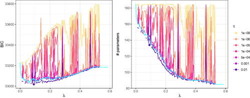
Figure 7 shows the BIC as well as the number of parameters remaining in the model. Note that, consistent with findings by Orzek and Voelkle (2023) in continuous time SEM, the model selection is highly susceptible to the thresholding parameter τ. That is, depending on the optimization routine and threshold parameter setting used, researchers may come to different conclusions regarding the number of non-zero parameters. In Appendix D, we additionally provide parameter estimates for the loadings matrices of the specialized optimizer and three selected approximate solutions of the general purpose optimizer. Therein, we also present a comparison to the approximate solutions returned by the current version of regsem (package version 1.9.3) using the default general purpose optimizer. Similar to the results shown in Figure 7, Figure D3 in Appendix D shows that the threshold parameter τ has a considerable influence on the parameters returned by the regsem package.

Our empirical example provided the first evidence that the threshold parameter τ can affect the final parameter estimates in regularized SEM, both when using the newly developed package lessSEM as well as when using the established package regsem. In the next section, we will systematize these findings in a simulation study.

6. Simulation Study

To systematically compare general purpose optimizers and specialized optimizers, we ran a simulation study where we used lasso regularization to identify non-zero cross-loadings in a confirmatory factor analysis (see also Huang et al., 2017; Scharf & Nestler, 2019). We used a three factor CFA as population model, defining the model and its population parameter values as follows:⁷ (4) $$\left[\begin{array}{c}{y}_1\\ y_2\\ y_3\\ y_4\\ y_5\\ y_6\\ y_7\\ y_8\\ y_9\\ y_{10}\\ y_{11}\\ y_{12}\\ y_{13}\\ y_{14}\\ y_{15}\end{array}\right]=\left[\begin{array}{ccc}\underset{¯}{1}& 0.291& 0\\ \underset{¯}{0.858}& 0& 0\\ \underset{¯}{0.782}& 0& 0.129\\ \underset{¯}{0.877}& 0& 0.293\\ \underset{¯}{0.888}& 0& 0\\ 0& \underset{¯}{1}& 0.28\\ 0& \underset{¯}{0.815}& 0\\ 0& \underset{¯}{0.721}& 0\\ 0.206& \underset{¯}{0.88}& 0\\ 0.109& \underset{¯}{0.749}& 0\\ 0.278& 0& \underset{¯}{1}\\ 0& 0& \underset{¯}{0.842}\\ 0& 0& \underset{¯}{0.809}\\ 0& 0.108& \underset{¯}{0.819}\\ 0& 0.166& \underset{¯}{0.758}\end{array}\right]\left[\begin{array}{c}{\xi }_1\\ {\xi }_2\\ {\xi }_3\end{array}\right]+\mathit{\epsilon }$$(4) (5) $$\mathit{\varphi }=\text{diag}(1,1,1)$$(5) (6) $$\begin{array}{c}{\mathbf{\Theta }}_{\mathit{\epsilon }}=\text{diag}(0.115,0.464,0.572,0.345,0.411,0.122,0.536,\\ 0.68,0.383,0.627,0.123,0.491,0.546,0.518,0.598)\end{array}$$(6)

Equation (4)(4) $$\left[\begin{array}{c}{y}_1\\ y_2\\ y_3\\ y_4\\ y_5\\ y_6\\ y_7\\ y_8\\ y_9\\ y_{10}\\ y_{11}\\ y_{12}\\ y_{13}\\ y_{14}\\ y_{15}\end{array}\right]=\left[\begin{array}{ccc}\underset{¯}{1}& 0.291& 0\\ \underset{¯}{0.858}& 0& 0\\ \underset{¯}{0.782}& 0& 0.129\\ \underset{¯}{0.877}& 0& 0.293\\ \underset{¯}{0.888}& 0& 0\\ 0& \underset{¯}{1}& 0.28\\ 0& \underset{¯}{0.815}& 0\\ 0& \underset{¯}{0.721}& 0\\ 0.206& \underset{¯}{0.88}& 0\\ 0.109& \underset{¯}{0.749}& 0\\ 0.278& 0& \underset{¯}{1}\\ 0& 0& \underset{¯}{0.842}\\ 0& 0& \underset{¯}{0.809}\\ 0& 0.108& \underset{¯}{0.819}\\ 0& 0.166& \underset{¯}{0.758}\end{array}\right]\left[\begin{array}{c}{\xi }_1\\ {\xi }_2\\ {\xi }_3\end{array}\right]+\mathit{\epsilon }$$(4) shows the measurement model, where we assumed that the core of the three latent factors (ξ₁, ξ₂, ξ₃) is reflected by five items each. Loadings on these items are underlined in Equation (4)(4) $$\left[\begin{array}{c}{y}_1\\ y_2\\ y_3\\ y_4\\ y_5\\ y_6\\ y_7\\ y_8\\ y_9\\ y_{10}\\ y_{11}\\ y_{12}\\ y_{13}\\ y_{14}\\ y_{15}\end{array}\right]=\left[\begin{array}{ccc}\underset{¯}{1}& 0.291& 0\\ \underset{¯}{0.858}& 0& 0\\ \underset{¯}{0.782}& 0& 0.129\\ \underset{¯}{0.877}& 0& 0.293\\ \underset{¯}{0.888}& 0& 0\\ 0& \underset{¯}{1}& 0.28\\ 0& \underset{¯}{0.815}& 0\\ 0& \underset{¯}{0.721}& 0\\ 0.206& \underset{¯}{0.88}& 0\\ 0.109& \underset{¯}{0.749}& 0\\ 0.278& 0& \underset{¯}{1}\\ 0& 0& \underset{¯}{0.842}\\ 0& 0& \underset{¯}{0.809}\\ 0& 0.108& \underset{¯}{0.819}\\ 0& 0.166& \underset{¯}{0.758}\end{array}\right]\left[\begin{array}{c}{\xi }_1\\ {\xi }_2\\ {\xi }_3\end{array}\right]+\mathit{\epsilon }$$(4) and will be referred to as core-loadings in the following. Among these core-loadings, one was set to 1; this loading was used for scaling the latent variables in the analysis.⁸ All other core-loadings were drawn from the uniform distribution ${\mathcal{U}}_{[0.7,0.9]}.$ Additionally, we allowed for three non-zero cross-loadings per latent factor. The location of these cross-loadings was randomly selected and their values drawn from ${\mathcal{U}}_{[0.1,0.3]}.$ The variances of the three factors was set to one (see Equation 5(5) $$\mathit{\varphi }=\text{diag}(1,1,1)$$(5) ; the diag $(·)$ operator populates the diagonal of a square zero matrix with the embraced values) and the variances of the residuals was set such that the overall-variance of each manifest variable was 1.2 (see Equation 6(6) $$\begin{array}{c}{\mathbf{\Theta }}_{\mathit{\epsilon }}=\text{diag}(0.115,0.464,0.572,0.345,0.411,0.122,0.536,\\ 0.68,0.383,0.627,0.123,0.491,0.546,0.518,0.598)\end{array}$$(6) ). Because all items have the same expected variance no further standardization is required.

We simulated five hundred data sets with a sample size of N = 250 and fitted unregularized and regularized models with R (R Core Team, 2022) using lavaan (Rosseel, 2012) and lessSEM. We estimated both core- and cross-loadings freely with the exception of the first core-loading of each latent variable which we set to 1 for scaling. All cross-loadings were regularized with the lasso penalty. For the tuning parameter λ, we generated 200 evenly spaced values between 0 and the first λ that zeroed all regularized parameters. In case of the general purpose optimizer, we either ignored the non-differentiability or smoothed the lasso penalty with $ϵ\in \{{10}^{-8},{10}^{-6},{10}^{-4},{10}^{-2}\}$ and estimated the parameters with the BFGS procedure outlined in Appendix A. We stopped the optimization if the GLMNET criterion outlined in Yuan et al. (2012, see Equation 25) was met for both, general purpose and specialized optimization. The only exception was the combination of general purpose optimizer and ignored non-differentiability, where we treated the model as converged if the change in fit from one iteration to the next fell below the threshold ${10}^{-6}.$ This exception was made due to the long runtimes when using the gradient-based GLMNET criterion. Average run times were between 4.4 (general purpose optimization with $ϵ={10}^{-2}$) and 11.8 s (general purpose optimization when ignoring the non-differentiability). In the following, we will compare the results of the general purpose optimizer and the specialized optimizer for the two steps of estimating a regularized SEM separately. This will shed light on the roots of the differences observed in the empirical example.

6.1. Differences in Step One: Estimating Increasingly Sparse Models

We first checked if both optimization routines—the general purpose optimizer and the specialized optimizer—performed similarly in terms of minimizing $F_{\text{reg},\lambda }(\mathit{\theta }).$ To this end, we defined the relative fit (RF) for repetition $r\in \{1,2,\dots ,500\}$ as (7) $${\text{RF}}_{r,\lambda ,ϵ}=\frac{F_{\text{reg},\lambda ,r}\left({\widehat{\mathit{\theta }}}_{\lambda ,r,ϵ}^a\right)}{F_{\text{reg},\lambda ,r}\left({\widehat{\mathit{\theta }}}_{\lambda ,r}^e\right)},$$(7) where $F_{\text{reg},\lambda ,r}(·)$ is the value of the regularized fitting function in repetition r for a given λ. The vector ${\widehat{\mathit{\theta }}}_{\lambda ,r,ϵ}^a$ holds approximate parameter estimates returned by the general purpose optimizer for a given smoothing parameter ϵ. Similarly, ${\widehat{\mathit{\theta }}}_{\lambda ,r}^e$ is a vector with exact parameter estimates produced by the specialized optimizer. A value of 1.02, for example, indicates that the approximate solution of the general purpose optimizer resulted in a 2% larger (i.e., worse) fitting function value than the exact solution of the specialized optimizer. Values below 1, in contrast, indicate that the general purpose optimizer outperformed the specialized optimizer.

Additionally, we computed the sum of the squared differences (SSD) between the parameter estimates of the general purpose optimizer and the specialized optimizer. The SSD was defined as: (8) $${\text{SSD}}_{\lambda ,r,ϵ}={\left({\widehat{\mathit{\theta }}}_{\lambda ,r,ϵ}^a-{\widehat{\mathit{\theta }}}_{\lambda ,r}^e\right)}^{\top }\left({\widehat{\mathit{\theta }}}_{\lambda ,r,ϵ}^a-{\widehat{\mathit{\theta }}}_{\lambda ,r}^e\right).$$(8)

Larger values indicate larger differences between the general purpose optimizer and the specialized optimizer.

Figure 8 shows the relative fit of the approximate solutions with the general purpose optimizer as compared to the exact solutions of the specialized optimizer. Note that the specialized optimizer almost always resulted in a better fit than the general purpose optimizer. However, the differences were negligible in many cases. Ignoring the non-differentiability resulted in a worse fit, which may have been due to issues with the gradient computation. Furthermore, smoothing the penalty function worked better with smaller ϵ values.

Figure 9 shows the SSD. Notably, the differences in the fitting function values are also reflected in differences in the parameter estimates. To provide additional insights into the roots of the differences observed in Figure 9, we plotted the regularized parameter estimates returned by the general purpose optimizer and the specialized optimizer for the first of the 500 repetitions in Figure 10. Note that (1) larger ϵ values result in slower shrinkage toward zero and (2) ignoring the non-differentiability results in more “ragged” paths, indicating that the optimizer may have had difficulties finding a minimum.

Overall, our results suggest that approximate solutions based on general purpose optimizers with smoothed penalty functions and exact solutions using a specialized optimizer perform similarly in terms of model fit and SSD if ϵ is set carefully. Importantly, however, model selection is not yet taken into account in these comparisons. In practice, only the parameter estimates of the final model (i.e., a specific λ value) are of relevance. For this reason, we now turn to model selection and repeat the comparison for the final model as selected by the BIC.

6.2. Differences in Step Two: Selecting the Best Model

To test the model selection with the BIC, we set the threshold parameter τ to $\tau \in \{{10}^{-8},{10}^{-6},{10}^{-5},{10}^{-4},5\times {10}^{-3},{10}^{-3},{10}^{-2}\}.$⁹ Additionally, we also used 5-fold cross-validation instead of the BIC to select the final model. Because cross-validation does not require zeroed parameters to improve, no threshold parameter τ is needed (τ was introduced because the BIC only improves if some parameters are set to exactly zero).

The selected models were again compared to the exact solution provided by the specialized optimizer using the SSD defined in Equation (9)(9) $${\text{SSD}}_{r,ϵ,\tau }={\left({\widehat{\mathit{\theta }}}_{r,ϵ,\tau }^a-{\widehat{\mathit{\theta }}}_r^e\right)}^{\top }\left({\widehat{\mathit{\theta }}}_{r,ϵ,\tau }^a-{\widehat{\mathit{\theta }}}_r^e\right).$$(9) . (9) $${\text{SSD}}_{r,ϵ,\tau }={\left({\widehat{\mathit{\theta }}}_{r,ϵ,\tau }^a-{\widehat{\mathit{\theta }}}_r^e\right)}^{\top }\left({\widehat{\mathit{\theta }}}_{r,ϵ,\tau }^a-{\widehat{\mathit{\theta }}}_r^e\right).$$(9)

Here, ${\widehat{\mathit{\theta }}}_{r,ϵ,\tau }^a$ and ${\widehat{\mathit{\theta }}}_r^e$ are the final parameter estimates for the general purpose and specialized optimizer, respectively. In case of the general purpose optimizer, the final parameter estimate depends on both smoothing parameter ϵ and threshold parameter τ. Again, larger SSD indicate larger differences between the approximate optimizer and the specialized optimizer.

Because model sparsity is often a motivation for using LASSO regularization, we also investigated the differences in the number of parameters t remaining in the model ($\Delta t_{r,ϵ,\tau }$): (10) $$\Delta t_{r,ϵ,\tau }=\sum _{j=1}^J\mathbb{1}({\widehat{\theta }}_{r,ϵ,\tau ,j}^a\ne 0)\text{-}\mathrm{ }\mathbb{1}({\widehat{\theta }}_{r,j}^e\ne 0)$$(10)

Here, J is the length of parameter vector $\mathit{\theta },\mathbb{1}(·)$ is an indicator function that returns one if the embraced condition is met and zero otherwise, and ${\widehat{\theta }}_{r,ϵ,\tau ,j}^a$ is the j-th element of vector ${\widehat{\theta }}_{r,ϵ,\tau }^a.$ A $\Delta t_{r,ϵ,\tau }$ of one, for instance, indicates that the approximate solution of the general purpose optimizer has one parameter more than the exact solution of the specialized optimizer. That is, researchers may come to different conclusions depending on which of the two optimization procedures they used. The difference $\Delta t_{r,ϵ,\tau }$ was not computed in case of cross-validation as cross-validation does not use τ and therefore none of the parameters will be set to zero in case of general purpose optimization.

Figure 11 shows the SSD of the final parameter estimates of the approximate solutions provided by the general purpose optimizer compared to the exact solutions provided by the specialized optimizer across all 500 simulation runs when using the BIC to select the final models. As expected, τ clearly affected the model selection. If τ is very small, the selected approximate solution was often the maximum likelihood estimates ${\widehat{\mathit{\theta }}}_{\text{ML}}.$ This is because the regularized estimates rarely fell below τ and therefore no improvement in the BIC was observed. Moreover, τ also interacted with ϵ in the smoothed penalty functions such that, for instance, $\tau =5\times {10}^{-4}$ worked well when $ϵ={10}^{-8},$ but not with $ϵ={10}^{-4}.$ Smaller ϵ values typically resulted in regularized estimates which are closer to zero and thus more likely to fall below a small threshold τ (this follows from Figure 10, where larger ϵ resulted in slower convergence to zero). Ignoring the non-differentiability performed worse than smoothing the penalty function with a small ϵ.

Figure 12 shows the SSD when using 5-fold cross-validation to select the final model. The model selection was considerably more consistent between both general purpose optimization and specialized optimization. However, none of the parameters is exactly zero in case of the general purpose optimization, which may impact the interpretation of the model (e.g., Orzek & Voelkle, 2023).

Figure 13 shows the difference in the number of parameters remaining in the model ($\Delta t_{r,ϵ,\tau }$) when using the BIC to select the final model. Importantly, general purpose optimization could result in a very different number of parameters, even in the best settings tested here. As non-zeroed parameter estimates are considered to be important (e.g., Jacobucci et al., 2019), this may also affect the conclusions drawn from the final model.

Overall, our results show that relatively small differences in the two additional tuning parameters—ϵ and τ—can alter the results substantially. For us, the only way to tell which combination works best was to implement both, a general purpose optimizer and a specialized optimizer. For the BFGS procedure used here, the combination of $ϵ={10}^{-8}$ and $\tau =5\times {10}^{-4}$ performed fairly well.

7. Discussion

The objective of this work was to systematically test the differences between general purpose optimizers and specialized optimizers as currently used in regularized SEM in order to shed light on differences observed between regsem and lslx. To this end, we compared both, the fit and the parameter estimates of regularized SEM with two similar optimization strategies: A quasi-Newton optimizer for smooth fitting functions (BFGS) and a quasi-Newton optimizer for non-smooth fitting functions (GLMNET). Ignoring model selection, we found that (1) differences in the fit and the parameter estimates between both optimization procedures are often negligible. However, (2) when combined with information criteria, as currently used in regsem, even small differences can result in unstable model selection. Only if both tuning parameters of general purpose optimizers—the smoothing parameter ϵ and the threshold parameter τ—are well selected can we expect similar results.

Our results are consistent with Orzek and Voelkle (2023), who found that the threshold parameter τ is critical in regularized continuous-time SEM. Moreover, we revealed an interaction of ϵ and τ: Specific combinations for ϵ and τ may exist for which the differences between approximate and exact solutions are small. In practice, however, these settings are unknown and, as our simulation demonstrated, may fail for any given data set. Importantly, the combination that worked best for the general purpose optimizer used in our simulations may not generalize to, for instance, regsem, where SEMs are implemented differently and other optimizers are used. Furthermore, our simulations showed that ignoring the non-differentiability can result in worse parameter estimates than a smoothly approximated penalty. Overall, this suggests that researchers using approximate solutions should be cautious when selecting models by means of information criteria.

On the other hand, our results showed that cross-validation is a viable alternative to using information criteria with approximate solutions. Importantly, no threshold parameter τ is required when using cross-validation for model selection. However, cross-validation is time consuming and may therefore be impractical for some models.

A promising alternative is to adapt the computation of the number of parameters t in the BIC (e.g., Geminiani et al., 2021; Muggeo, 2010; Ulbricht, 2010). The approximation strategy proposed by Geminiani et al. (2021) and based on Ulbricht (2010), for instance, uses the generalized information criterion (Konishi & Kitagawa, 1996). This approach does not require the threshold parameter τ and is implemented in the R package penfa (Geminiani et al., 2021) for confirmatory factor analyses. However, to the best of our knowledge, this approximation strategy has not yet been extended to SEM. Additionally, the specific approximations proposed by Geminiani et al. (2021) are fairly involved, reducing the simplicity-advantage of implementing approximate solutions. On the other hand, Geminiani et al. (2021) also proposed confidence intervals and an automatic tuning parameter selection for their approximation. Extending this approach to SEM, therefore, appears promising. Alternatively, procedures may be developed that allow for a more sophisticated threshold parameter τ (see e.g., Cao et al., 2017, for such a procedure in group bridge penalized regression). Finally, for a different smooth approximation, Muggeo (2010) found that their smoothing parameter c can have a considerable effect on the model selection even if an adapted computation for the number of parameters t is used. This should be considered when implementing such approximations.

On a final note, our findings are most likely not limited to regularized SEM: Other regularized models may also be fitted with either general purpose or specialized optimizers. However, the situation in regularized SEM is special in that one of the most popular implementations of regularized SEM to date relies on the combination of a general purpose optimizer for estimation and the BIC for model selection by default. Other packages for regularized estimation use specialized optimizers instead (e.g., lslx, Huang, 2020a; glmnet, Friedman et al., 2010; ncvreg, Breheny & Huang, 2011, or LIBLINEAR, Fan et al., 2008). Thus, while our findings may generalize to other models, they are of central importance to the regularization of SEM.

Our study comes with several limitations. First, we only looked at the lasso penalty. One may therefore wonder if the results generalize to the wealth of other penalty functions proposed in the literature, such as the adaptive lasso (Zou, 2006), elastic net (Zou & Hastie, 2005), scad (Fan & Li, 2001), lsp (Candès et al., 2008), cappedL1 (Zhang, 2010), and mcp (Zhang, 2010). Importantly, all of the penalties mentioned above use the absolute value function to obtain sparse solutions. Replacing this absolute value function with an approximation, as done for the lasso penalty in this study, results in non-sparse solutions and requires the threshold parameter τ. Still, more in-depth analyses for these penalty functions may be worthwhile given that they also come with additional tuning parameters besides λ. Second, we did not compare the final parameter estimates of the general purpose optimizer and the specialized optimizer to the true parameters used in the simulation. The reason for this is that the objective of the approximation used in the general purpose optimizer is to return parameter estimates, which are as close as possible to the exact solution of the specialized optimizer. Outperforming exact solutions is not the reason for existence of the approximation. And even if approximate solutions would outperform exact solutions for some specific settings of ϵ and τ, this may just reflect that approximate solutions have more tuning parameters. Making use of these tuning parameters would require optimizing models for an entire tuning grid (combinations of all λ, ϵ, and τ values), resulting in a considerable increase in run time. This is especially true because τ cannot be selected with information criteria.¹⁰ Third, we restricted our analyses to models fitted with lessSEM using two optimizers only (BFGS and GLMNET). These optimizers were selected because of their popularity and similarity due to both employing quasi-Newton procedures. However, it remains unclear if the results generalize to other optimizers as well.

All in all, we conclude that specialized optimizers should be preferred over general purpose optimizers in regularized SEM when using the current implementations of information criteria to select the final parameter estimates. These specialized optimizers are the default in lslx and lessSEM, and optionally available in regsem. When developing new regularized SEMs (e.g., models estimated with the Kalman filter), however, our results leave researchers between a rock and a hard place. General purpose optimizers are widely available and therefore easier to implement but may result in questionable model selection if standard information criteria are used. Implementing specialized optimizers, on the other hand, is time consuming and error prone. Here, lessSEM can provide a starting point because all optimizers implemented therein can be accessed using both, R and C++ (see Appendix C for an example). In addition to the lasso penalty discussed above, researchers using lessSEM also have access to optimizers for all other penalty functions mentioned in the introduction (namely ridge, adaptive lasso, elastic net, cappedL1, lsp, scad, and mcp). Combined with the additional features of lessSEM (full information maximum likelihood estimation, multi-group models, definition variables, parameters transformations, and mixtures of penalties), this allows for the rapid development of new regularized models.

Acknowledgments

During the work on his dissertation, Jannik H. Orzek was a pre-doctoral fellow of the International Max Planck Research School on the Life Course (https://www.imprs-life.mpg.de/) of the Max Planck Institute for Human Development, Berlin, Germany. We acknowledge support by the Open Access Publication Fund of Humboldt-Universität zu Berlin. Figures in this article were created with ggplot2 (Wickham, 2016) and ggdist (Kay, 2022). The online supplement can be found at https://osf.io/kh9tr/.

Notes

1 For instance, lslx offers multi-group regularization, whereas regsem allows for equality constraints of parameters.

2 The gradient is a vector of first derivatives of the fitting function with respect to the parameters and the Hessian is a matrix with second derivatives.

3 The threshold parameter τ can be adapted with the round parameter in regsem; see regsem-function in the regsem package.

4 The lessSEM (lessSEM estimates sparse SEM) version used in this study is available from https://osf.io/kh9tr/. The most recent version can be found at https://github.com/jhorzek/lessSEM. Similar to regsem, lessSEM builds on models from lavaan (Rosseel, 2012).

5 We compare our implementation with lslx in the osf repository at https://osf.io/kh9tr/.

6 See fasta (Goldstein et al., 2016) for an alternative R package implementing general purpose optimization of non-differentiable penalty functions in pure R.

7 Files to replicate the simulations and the empirical example are provided in the osf repository at https://osf.io/kh9tr/. All analyses were performed using a single core of an Intel^® Xeon^® E5-2670 processor.

8 We chose this way of scaling because scaling by setting the variances to 1 would allow for multiple equivalent solutions with reversed signs of loadings.

9 In regsem $\tau ={10}^{-3}$ is the current default, while Belzak and Bauer (2020) and Epskamp et al. (2017) used $\tau ={10}^{-5}.$

10 The best BIC, for example, would always be achieved by setting $\tau =\infty$ and λ = 0. Then, the BIC reduces to $F_{\text{ML}}({\widehat{\mathit{\theta }}}_{\text{ML}})$ (the −2 log-likelihood of the maximum likelihood parameter estimates) plus $\hspace{0.17em}\log \hspace{0.17em}(N)$ times the number of unregularized parameters.

 

Appendix A

A.1 A Short Introduction to Quasi-Newton Optimization

Assume that $F_{\text{reg},\lambda }(\mathit{\theta })$ is twice continuously differentiable and that in iteration k we are at the point ${\mathit{\theta }}_k.$ Points of $F_{\text{reg},\lambda }(\mathit{\theta })$ close to ${\mathit{\theta }}_k$ are approximated using a truncated Taylor series: (A.1) $$\begin{array}{cc}{F}_{\text{reg},\lambda }(\mathit{\theta })\approx \hfill & F_{\text{reg},\lambda }({\mathit{\theta }}_k)\hfill \\ \hfill & +(\mathit{\theta }-{\mathit{\theta }}_k){▽}_{\mathit{\theta }}{F}_{\text{reg},\lambda }({\mathit{\theta }}_k)\hfill \\ \hfill & +\frac{1}{2}(\mathit{\theta }-{\mathit{\theta }}_k){▽}_{\mathit{\theta }}^2{F}_{\text{reg},\lambda }({\mathit{\theta }}_k){(\mathit{\theta }-{\mathit{\theta }}_k)}^{\top }.\hfill \end{array}$$(A.1)

Here, ${▽}_{\mathit{\theta }}{F}_{\text{reg},\lambda }({\mathit{\theta }}_k)$ is the gradient of the function at point ${\mathit{\theta }}_k$ and ${▽}_{\mathit{\theta }}^2{F}_{\text{reg},\lambda }({\mathit{\theta }}_k)$ is the Hessian. If the Hessian ${▽}_{\mathit{\theta }}^2{F}_{\text{reg},\lambda }({\mathit{\theta }}_k)$ is positive definite, Equation (A.1)(A.1) $$\begin{array}{cc}{F}_{\text{reg},\lambda }(\mathit{\theta })\approx \hfill & F_{\text{reg},\lambda }({\mathit{\theta }}_k)\hfill \\ \hfill & +(\mathit{\theta }-{\mathit{\theta }}_k){▽}_{\mathit{\theta }}{F}_{\text{reg},\lambda }({\mathit{\theta }}_k)\hfill \\ \hfill & +\frac{1}{2}(\mathit{\theta }-{\mathit{\theta }}_k){▽}_{\mathit{\theta }}^2{F}_{\text{reg},\lambda }({\mathit{\theta }}_k){(\mathit{\theta }-{\mathit{\theta }}_k)}^{\top }.\hfill \end{array}$$(A.1) has the minimum $-{▽}_{\mathit{\theta }}^2{F}_{\text{reg},\lambda }{({\mathit{\theta }}_k)}^{-1}{▽}_{\mathit{\theta }}{F}_{\text{reg},\lambda }({\mathit{\theta }}_k)$ which is used as step direction ${\mathit{d}}_k$ (so-called Newton direction; Nocedal & Wright, 2006). In this case, the step of length s_k is typically set to 1. Figure 2 shows such Newton steps, with the blue lines depicting the approximations using Equation (A.1)(A.1) $$\begin{array}{cc}{F}_{\text{reg},\lambda }(\mathit{\theta })\approx \hfill & F_{\text{reg},\lambda }({\mathit{\theta }}_k)\hfill \\ \hfill & +(\mathit{\theta }-{\mathit{\theta }}_k){▽}_{\mathit{\theta }}{F}_{\text{reg},\lambda }({\mathit{\theta }}_k)\hfill \\ \hfill & +\frac{1}{2}(\mathit{\theta }-{\mathit{\theta }}_k){▽}_{\mathit{\theta }}^2{F}_{\text{reg},\lambda }({\mathit{\theta }}_k){(\mathit{\theta }-{\mathit{\theta }}_k)}^{\top }.\hfill \end{array}$$(A.1) at the points θ₁, θ₂, θ₃, and θ₄. However, computing the true Hessian is often prohibitively expensive and one may resort to an approximation thereof. In lessSEM, we use the Broyden–Fletcher–Goldfarb–Shanno (BFGS) approximation (see e.g., Nocedal & Wright, 2006), resulting in a quasi-Newton procedure. When approximating the Hessian, s_k = 1 may be a poor choice and the best step length is therefore found in a second optimization (e.g., Nocedal & Wright, 2006). To increase the similarity between the quasi-Newton optimizer outlined here and the GLMNET optimizer introduced in the next section, we used the same procedure to find the step size s_k: We decreased s until the criterion shown in Equation (A.2)(A.2) $$F_{\text{reg},\lambda }({\mathit{\theta }}_k+s{\mathit{d}}_k)\le F_{\text{reg},\lambda }({\mathit{\theta }}_k)+s\sigma {▽}_{\mathit{\theta }}{F}_{\text{reg},\lambda }{({\mathit{\theta }}_k)}^{\top }{\mathit{d}}_k$$(A.2) was met, where $\sigma =0.1.$ This criterion is a simplification of the criterion proposed by Yuan et al. (2012) for GLMNET, where we take the differentiability of the approximated penalty into account. In fact, Equation (A.2)(A.2) $$F_{\text{reg},\lambda }({\mathit{\theta }}_k+s{\mathit{d}}_k)\le F_{\text{reg},\lambda }({\mathit{\theta }}_k)+s\sigma {▽}_{\mathit{\theta }}{F}_{\text{reg},\lambda }{({\mathit{\theta }}_k)}^{\top }{\mathit{d}}_k$$(A.2) is identical to the Armijo condition used by many optimizers (e.g., Nocedal & Wright, 2006, p. 33). (A.2) $$F_{\text{reg},\lambda }({\mathit{\theta }}_k+s{\mathit{d}}_k)\le F_{\text{reg},\lambda }({\mathit{\theta }}_k)+s\sigma {▽}_{\mathit{\theta }}{F}_{\text{reg},\lambda }{({\mathit{\theta }}_k)}^{\top }{\mathit{d}}_k$$(A.2)

Note that Equation (A.2)(A.2) $$F_{\text{reg},\lambda }({\mathit{\theta }}_k+s{\mathit{d}}_k)\le F_{\text{reg},\lambda }({\mathit{\theta }}_k)+s\sigma {▽}_{\mathit{\theta }}{F}_{\text{reg},\lambda }{({\mathit{\theta }}_k)}^{\top }{\mathit{d}}_k$$(A.2) enforces a decrease in $F_{\text{reg},\lambda }({\mathit{\theta }}_k)$ from one iteration to the next. This follows from $${▽}_{\mathit{\theta }}{F}_{\text{reg},\lambda }{({\mathit{\theta }}_k)}^{\top }{\mathit{d}}_k=-{▽}_{\mathit{\theta }}{F}_{\text{reg},\lambda }{({\mathit{\theta }}_k)}^{\top }{\mathit{H}}^{-1}{▽}_{\mathit{\theta }}{F}_{\text{reg},\lambda }({\mathit{\theta }}_k)\le 0$$

The matrix H is a positive definite (approximation of the) Hessian matrix. The inequality follows from (1) H being positive definite and therefore ${\mathit{H}}^{-1}$ being positive definite and (2) the definition of a positive definite matrix as a matrix M, where ${\mathit{x}}^{\top }\mathit{Mx}>0$ for any non-zero vector x (e.g., Petersen & Pedersen, 2012, pp. 50–51).

 

Appendix B

B.1 A Short Introduction to the GLMNET Optimizer

We will restrict the presentation of the GLMNET optimizer to a short primer. A thorough derivation is provided in the original publications (see Friedman et al., 2010; Yuan et al., 2012). We also recommend reading Appendix A before, as the quasi-Newton optimizer presented therein provides more background information on the general ideas used in the following. The GLMNET optimizer is also implemented in lslx (Huang, 2020a) and regCtsem (Orzek & Voelkle, 2023).

GLMNET is based on the assumption that the maximum likelihood fitting function $F_{\text{ML}}(\mathit{\theta })$ in Equation (1)(1) $$F_{\text{reg},\lambda }(\mathit{\theta })=F_{\text{ML}}(\mathit{\theta })+\lambda Np(\mathit{\theta })$$(1) is at least twice differentiable. Then, $F_{\text{reg},\lambda }(\mathit{\theta })$ can be approximated with (B.1) $$\begin{array}{cc}{F}_{\text{reg},\lambda }(\mathit{\theta })\approx \hfill & F_{\text{ML},\lambda }({\mathit{\theta }}_k)\hfill \\ \hfill & +(\mathit{\theta }-{\mathit{\theta }}_k){▽}_{\mathit{\theta }}{F}_{\text{ML},\lambda }({\mathit{\theta }}_k)\hfill \\ \hfill & +\frac{1}{2}(\mathit{\theta }-{\mathit{\theta }}_k){▽}_{\mathit{\theta }}^2{F}_{\text{ML},\lambda }({\mathit{\theta }}_k){(\mathit{\theta }-{\mathit{\theta }}_k)}^{\top }\hfill \\ \hfill & +\lambda p(\mathit{\theta }).\hfill \end{array}$$(B.1)

Note that the penalty function $p(\mathit{\theta })$ is not approximated in Equation (B.1)(B.1) $$\begin{array}{cc}{F}_{\text{reg},\lambda }(\mathit{\theta })\approx \hfill & F_{\text{ML},\lambda }({\mathit{\theta }}_k)\hfill \\ \hfill & +(\mathit{\theta }-{\mathit{\theta }}_k){▽}_{\mathit{\theta }}{F}_{\text{ML},\lambda }({\mathit{\theta }}_k)\hfill \\ \hfill & +\frac{1}{2}(\mathit{\theta }-{\mathit{\theta }}_k){▽}_{\mathit{\theta }}^2{F}_{\text{ML},\lambda }({\mathit{\theta }}_k){(\mathit{\theta }-{\mathit{\theta }}_k)}^{\top }\hfill \\ \hfill & +\lambda p(\mathit{\theta }).\hfill \end{array}$$(B.1) . From iteration k to iteration k + 1, our objective is to make Equation (B.1)(B.1) $$\begin{array}{cc}{F}_{\text{reg},\lambda }(\mathit{\theta })\approx \hfill & F_{\text{ML},\lambda }({\mathit{\theta }}_k)\hfill \\ \hfill & +(\mathit{\theta }-{\mathit{\theta }}_k){▽}_{\mathit{\theta }}{F}_{\text{ML},\lambda }({\mathit{\theta }}_k)\hfill \\ \hfill & +\frac{1}{2}(\mathit{\theta }-{\mathit{\theta }}_k){▽}_{\mathit{\theta }}^2{F}_{\text{ML},\lambda }({\mathit{\theta }}_k){(\mathit{\theta }-{\mathit{\theta }}_k)}^{\top }\hfill \\ \hfill & +\lambda p(\mathit{\theta }).\hfill \end{array}$$(B.1) smaller; or formally, we search a direction vector $\mathit{d}=\mathit{\theta }-{\mathit{\theta }}_k$ which minimizes (B.2) $$\begin{array}{cc}{F}_{\text{reg},\lambda }(\mathit{\theta })-F_{\text{reg},\lambda }({\mathit{\theta }}_k)\approx \hfill & \underset{\approx F_{\text{reg},\lambda }(\mathit{\theta })}{\underbrace{F_{\text{ML},\lambda }({\mathit{\theta }}_k)+\mathit{d}{▽}_{\mathit{\theta }}{F}_{\text{ML},\lambda }({\mathit{\theta }}_k)+\frac{1}{2}\mathit{d}{▽}_{\mathit{\theta }}^2{F}_{\text{ML},\lambda }({\mathit{\theta }}_k){\mathit{d}}^{\top }+\lambda p({\mathit{\theta }}_k+\mathit{d})}}\hfill \\ \hfill & -\underset{=F_{\text{reg},\lambda }({\mathit{\theta }}_k)}{\underbrace{F_{\text{ML},\lambda }({\mathit{\theta }}_k)-\lambda p({\mathit{\theta }}_k)}}\hfill \\ =\hfill & \mathit{d}{▽}_{\mathit{\theta }}{F}_{\text{ML},\lambda }({\mathit{\theta }}_k)+\frac{1}{2}\mathit{d}{▽}_{\mathit{\theta }}^2{F}_{\text{ML},\lambda }({\mathit{\theta }}_k){\mathit{d}}^{\top }+\lambda p({\mathit{\theta }}_k+\mathit{d})-\lambda p({\mathit{\theta }}_k)\hfill \\ =\hfill & q(\mathit{d})\hfill \end{array}$$(B.2)

The new problem, minimizing $q(\mathit{d}),$ is then solved with a coordinate descent procedure (Yuan et al., 2012). To this end, a second optimization is used, where single elements of $\mathit{\theta }$ are updated iteratively. Broadly speaking, the procedure is similar to the simplified example developed in the main text. However, the details are beyond the scope of the current article and the interested reader is referred to Friedman et al. (2010) and Yuan et al. (2012). In lessSEM, we additionally replace the Hessian matrix with the BFGS approximation.

After finding step direction ${\mathit{d}}_k$ with the coordinate descent procedure, the step length s_k is found by decreasing s until the criterion in Equation (B.3)(B.3) $$F_{\text{reg},\lambda }({\mathit{\theta }}_k+s{\mathit{d}}_k)\le F_{\text{reg},\lambda }({\mathit{\theta }}_k)+s\sigma \left({▽}_{\mathit{\theta }}{F}_{\text{ML}}{({\mathit{\theta }}_k)}^{\top }{\mathit{d}}_k+{\displaystyle \sum _{j=1}^p{r}_j}|{\theta }_{k,j}+d_{k,j}|-{\displaystyle \sum _{j=1}^p{r}_j}\left|{\theta }_{k,j}\right|\right)$$(B.3) is met, where $\sigma =0.1$ (this criterion was proposed by Yuan et al., 2012 and is also used by Huang, 2020a): (B.3) $$F_{\text{reg},\lambda }({\mathit{\theta }}_k+s{\mathit{d}}_k)\le F_{\text{reg},\lambda }({\mathit{\theta }}_k)+s\sigma \left({▽}_{\mathit{\theta }}{F}_{\text{ML}}{({\mathit{\theta }}_k)}^{\top }{\mathit{d}}_k+{\displaystyle \sum _{j=1}^p{r}_j}|{\theta }_{k,j}+d_{k,j}|-{\displaystyle \sum _{j=1}^p{r}_j}\left|{\theta }_{k,j}\right|\right)$$(B.3)

For our purpose, the most important message is that the quasi-Newton optimizer presented in Appendix A and the GLMNET optimizer discussed here are similar in that they rely on truncated second order Taylor series approximations to $F_{\text{reg},\lambda }({\mathit{\theta }}_k).$ Both use the BFGS approximation for the Hessian matrix and rely on a similar procedure to find step size s_k.

 

Appendix C

C.1 Optimizing Lasso Regression with lessSEM

To demonstrate the specialized optimizers implemented in the lessSEM package, we use a linear regression example.

Table

library(lessSEM) #### Simulate data #### set.seed(123) N <- 100 # number of persons p <- 10 # number of predictors X <- matrix(rnorm(N*p), nrow = N, ncol = p) # design matrix b <- c(rep(1,5), rep(0,p-5)) # true regression weights y <- X%*%matrix(b,ncol = 1) + rnorm(N,0,.2) #### Create the unregularized fitting and gradient functions #### ls <- function(b,y,X,N){  return((.5/N)*sum((y - X%*%matrix(b,ncol = 1))^  2)) } gradLs <- function(b,y,X,N){  return(t((.5/N)*(-2.0*t(X) %*% y + 2.0*t(X)%*%X%*%matrix(b,ncol = 1)))) } # Starting values (Important: They must have names) bEst <- rep(0,p) names(bEst) <- paste0("b", 1:length(b)) #### Estimate the model #### out <- lessSEM::gpLasso(par = bEst, regularized = names(bEst), fn = ls, gr = gradLs, lambdas = .5, X = X, y = y, N = N) coef(out) # for comparison: library(glmnet) coef(glmnet(x = X, y = y, lambda = .5, intercept = FALSE, standardize = FALSE))[,1] # using scad instead: out <- lessSEM::gpScad(par = bEst, regularized = names(bEst), fn = ls, gr = gradLs, lambdas = .5, thetas = 2.1, X = X, y = y, N = N) coef(out)

 

Appendix D

D.1 Empirical Example

Figure 1. Parameter estimates for four different penalty functions (ridge, lasso, elastic net, and scad) for increasing values of λ. The dots represent the selected points of λ at which parameters were estimated.

D.1.1 Comparison to regsem

When fitting the model with regsem, we used the defaults of the cv_regsem function except for (1) setting mult.start = TRUE because we observed many non-convergent results otherwise (2) and adapting the round parameter to match the τ values used above. We removed all models for which regsem reported a non-zero convergence code, regsem returned negative variances, or the parameter estimates implied correlations between latent variables which were not in the interval $[-1,1].$ Figure D2 shows the relative fit for each τ (the results from regsem differ between τ values because mult.start = TRUE uses random starting values). Both packages resulted in nearly identical fit values. Figure D3 shows the BIC and the number of non-zero parameters for regsem and lessSEM. Despite the similarity in fit, both packages select different final parameter estimates.

Figure 2. Steps taken by an optimizer. The red line is the function we want to minimize. The dots indicate the steps taken during the optimization and the blue lines are the approximations generated at these points (see Appendix A). Each point θ_k is found by minimizing the approximation at the previous point ${\theta }_{k-1}.$

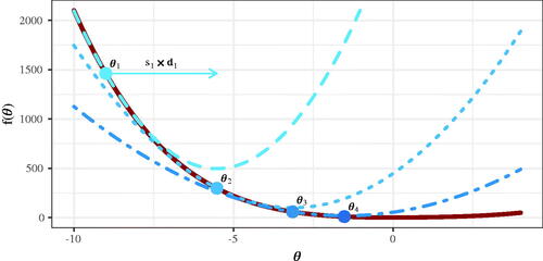
Figure 3. Penalty function values for a single parameter θ. The ridge is differentiable, whereas the lasso is not.

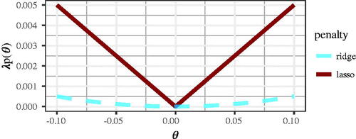
Figure 4. Penalty function values for a single parameter θ. Both, ridge and smoothed lasso are differentiable.

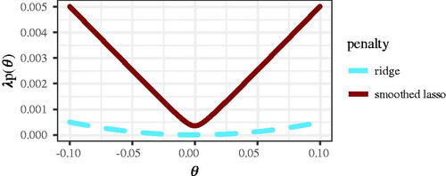
Figure 5. BIC for increasing λ values based on a single data set from the simulation study (see below). Dots indicate the discrete λ values for which models were fitted.

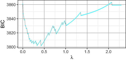
Figure 6. CFA for the bfi data set. Dashed blue paths are regularized cross-loadings.

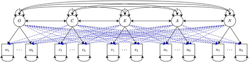
Figure 7. BIC and number of parameters for the N = 500 subset of the bfi data set when using approximate solutions (with the general purpose optimizer BFGS). The blue line is the exact solution (with the specialized optimizer GLMNET). Diamonds represent the respective selected models.

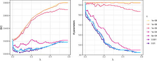
Figure 8. Quantile plots showing the relative fit. The quantiles were computed for each λ value separately. Values above 1 indicate better fit of the exact solution (using the specialized optimizer GLMNET), values below 1 indicate better fit of approximate solutions (using the general purpose optimizer BFGS). The black line shows the median. Values outside of the 95% quantile are not shown. A figure with all data points is included in the osf repository at https://osf.io/kh9tr/.

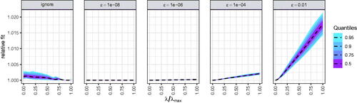
Figure 9. Quantile plots showing the sum of squared differences between exact solutions from the specialized optimizer and approximate solutions from the general purpose optimizer. Quantiles were computed for each λ separately. The black line shows the median. Values outside of the 95% quantile are not shown. A figure with all data points is included in the osf repository at https://osf.io/kh9tr/.

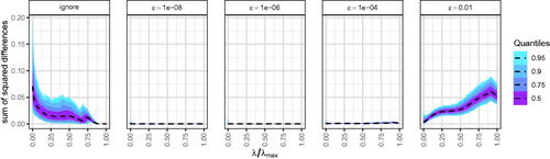
Figure 10. Regularized parameters estimates of the first repetition for exact solutions (using the specialized optimizer GLMNET) and approximate solutions (using the general purpose optimizer BFGS) for different levels of smoothing parameter ϵ.

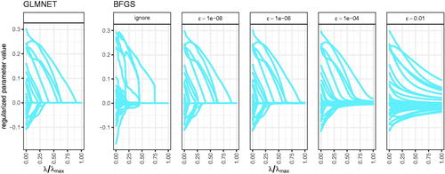
Figure 11. Sum of squared differences between exact solutions (using the specialized optimizer GLMNET) and approximate solutions (using the general purpose optimizer BFGS) in the final parameter estimates when using the BIC for model selection. Each dot represents one of the 500 simulation runs. Red dots indicate that the approximate solution selected the maximum likelihood estimates (i.e., $\widehat{\lambda }=0$).

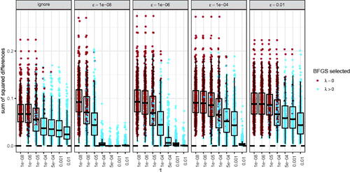
Figure 12. Sum of squared differences between exact solutions (using GLMNET) and approximate solutions (using BFGS) in the final parameter estimates when using 5-fold cross-validation for model selection.

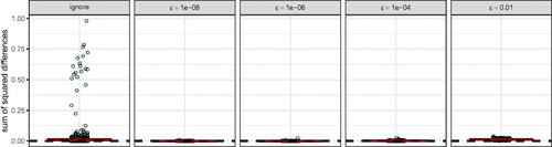
Figure 13. Difference in the number of non-zero parameter estimates between approximate and exact solutions when using the BIC for model selection. A value of 3, for instance, indicates that the approximate solution (using BFGS) has three more parameters than the exact solution (using GLMNET). Each dot represents one of the 500 simulation runs. Red dots indicate that the approximate solution selected the maximum likelihood estimates (i.e., λ = 0).

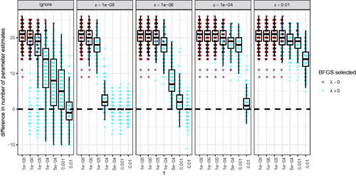
Figure D1. Final loadings estimated by exact (a) and approximate solutions (b–d) with different τ values. Results are rounded to three digits. Dots represent parameters which are either exactly zero (in case of exact solutions) or fall below the threshold τ.

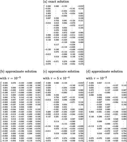
Figure D2. Relative fit of regsem as compared to lessSEM with GLMNET optimizer. A value of 1.01, for example, indicates a 1% larger fitting function value for regsem. The gaps represent non-convergent results based on (1) non-zero convergence codes, (2) negative variances, or (3) invalid correlations between latent variables in regsem.

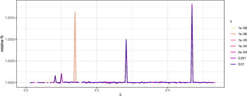
Figure D3. BIC and number of parameters for the bfi data set when using the regsem package. The blue line is the exact solution returned by lessSEM using the GLMNET optimizer. All other lines are the solutions returned by regsem using different levels of τ. Diamonds represent the respective selected models. The gaps in the BIC and the number of parameters for regsem represent non-convergent results based on (1) non-zero convergence codes, (2) negative variances, or (3) invalid correlations between latent variables.

References

- Andrew, G., & Gao, J. (2007). Scalable training of L1-regularized log-linear models. In Proceedings of the 24th International Conference on Machine Learning – ICML ’07 (pp. 33–40). ACM Press.
- Battauz, M. (2020). Regularized estimation of the nominal response model. Multivariate Behavioral Research, 55, 811–824. https://doi.org/10.1080/00273171.2019.1681252
- Belzak, W. C. M. (2021). Using regularization to evaluate differential item functioning among multiple covariates: A penalized expectation-maximization algorithm via coordinate descent and soft-thresholding [doctoral dissertation]. University of North Carolina, Chapel Hill.
- Belzak, W. C. M., & Bauer, D. J. (2020). Improving the assessment of measurement invariance: Using regularization to select anchor items and identify differential item functioning. Psychological Methods, 25, 673–690. https://doi.org/10.1037/met0000253
- Brandmaier, A. M., & Jacobucci, R. C. (in press). Machine-learning approaches to structural equation modeling. In R. H. Hoyle (Ed.), Handbook of structural equation modeling (2nd ed.). Guilford Press.
- Breheny, P., & Huang, J. (2011). Coordinate descent algorithms for nonconvex penalized regression, with applications to biological feature selection. The Annals of Applied Statistics, 5, 232–253. https://doi.org/10.1214/10-AOAS388
- Browne, M. W. (2000). Cross-validation methods. Journal of Mathematical Psychology, 44, 108–132. https://doi.org/10.1006/jmps.1999.1279
- Candès, E. J., Wakin, M. B., & Boyd, S. P. (2008). Enhancing sparsity by reweighted l1 minimization. Journal of Fourier Analysis and Applications, 14, 877–905. https://doi.org/10.1007/s00041-008-9045-x
- Cao, Y., Huang, J., Jiao, Y., & Liu, Y. (2017). A lower bound based smoothed quasi-Newton algorithm for group bridge penalized regression. Communications in Statistics-Simulation and Computation, 46, 4694–4707. https://doi.org/10.1080/03610918.2015.1129409
- Chamroukhi, F., & Huynh, B.-T. (2019). Regularized maximum likelihood estimation and feature selection in mixtures-of-experts models. Journal de la Société Française de Statistique, 160, 57–85.
- Davis, S. W., Szymanski, A., Boms, H., Fink, T., & Cabeza, R. (2019). Cooperative contributions of structural and functional connectivity to successful memory in aging. Network Neuroscience, 3, 173–194. https://doi.org/10.1162/netn_a_00064
- Eddelbuettel, D., & François, R. (2011). Rcpp: Seamless R and C++ integration. Journal of Statistical Software, 40, 1–18. https://doi.org/10.18637/jss.v040.i08
- Eddelbuettel, D., & Sanderson, C. (2014). RcppArmadillo: Accelerating R with high-performance C++ linear algebra. Computational Statistics & Data Analysis, 71, 1054–1063. https://doi.org/10.1016/j.csda.2013.02.005
- Epskamp, S., Rhemtulla, M., & Borsboom, D. (2017). Generalized network psychometrics: Combining network and latent variable models. Psychometrika, 82, 904–927. https://doi.org/10.1007/s11336-017-9557-x
- Fan, J., & Li, R. (2001). Variable selection via nonconcave penalized likelihood and its oracle properties. Journal of the American Statistical Association, 96, 1348–1360. https://doi.org/10.1198/016214501753382273
- Fan, R.-E., Chang, K.-W., Hsieh, C.-J., Wang, X.-R., & Lin, C.-J. (2008). LIBLINEAR: A library for large linear classification. Journal of Machine Learning Research, 9, 1871–1874.
- Finch, W. H., & Miller, J. E. (2021). A comparison of regularized maximum-likelihood, regularized 2-stage least squares, and maximum-likelihood estimation with misspecified models, small samples, and weak factor structure. Multivariate Behavioral Research, 56, 608–626. https://doi.org/10.1080/00273171.2020.1753005
- Friedman, J., Hastie, T., & Tibshirani, R. (2010). Regularization paths for generalized linear models via coordinate descent. Journal of Statistical Software, 33, 1–20. https://doi.org/10.18637/jss.v033.i01
- Friemelt, B., Bloszies, C., Ernst, M. S., Peikert, A., Brandmaier, A. M., & Koch, T. (2022). On the performance of different regularization methods in bifactor-(S-1) models with explanatory variables—Caveats, recommendations, and future directions. Structural Equation Modeling: A Multidisciplinary Journal. Advance online publication. https://doi.org/10.1080/10705511.2022.2140664
- Geminiani, E., Marra, G., & Moustaki, I. (2021). Single- and multiple-group penalized factor analysis: A trust-region algorithm approach with integrated automatic multiple tuning parameter selection. Psychometrika, 86, 65–95. https://doi.org/10.1007/s11336-021-09751-8
- Ghalanos, A., & Theussl, S. (2015). Rsolnp: General non-linear optimization using augmented lagrange multiplier method.
- Goldstein, T., Studer, C., & Baraniuk, R. (2016). A field guide to forward-backward splitting with a FASTA implementation (No. arXiv:1411.3406). arXiv.
- Gong, P., Zhang, C., Lu, Z., Huang, J., Ye, J. (2013). A general iterative shrinkage and thresholding algorithm for non-convex regularized optimization problems. In Proceedings of the 30th International Conference on Machine Learning (Vol. 28, pp. 37–45). PMLR.
- Góngora, D., Vega-Hernández, M., Jahanshahi, M., Valdés-Sosa, P. A., Bringas-Vega, M. L., & C. (2020). Crystallized and fluid intelligence are predicted by microstructure of specific white-matter tracts. Human Brain Mapping, 41, 906–916. https://doi.org/10.1002/hbm.24848
- Hastie, T., Tibshirani, R., & Wainwright, M. (2015). Statistical learning with sparsity: The lasso and generalizations. CRC Press.
- Hoerl, A. E., & Kennard, R. W. (1970). Ridge regression: Biased estimation for nonorthogonal problems. Technometrics, 12, 55–67. https://doi.org/10.1080/00401706.1970.10488634
- Huang, P.-H. (2018). A penalized likelihood method for multi-group structural equation modelling. British Journal of Mathematical and Statistical Psychology, 71, 499–522. https://doi.org/10.1111/bmsp.12130
- Huang, P.-H. (2020a). Lslx: Semi-confirmatory structural equation modeling via penalized likelihood. Journal of Statistical Software, 93, 1–37. https://doi.org/10.18637/jss.v093.i07
- Huang, P.-H. (2020b). Penalized least squares for structural equation modeling with ordinal responses. Multivariate Behavioral Research, 57, 279–297. https://doi.org/10.1080/00273171.2020.1820309
- Huang, P.-H., Chen, H., & Weng, L.-J. (2017). A penalized likelihood method for structural equation modeling. Psychometrika, 82, 329–354. https://doi.org/10.1007/s11336-017-9566-9
- Jacobucci, R. (2017). Regsem: Regularized structural equation modeling. arXiv:1703.08489 [stat].
- Jacobucci, R., Brandmaier, A. M., & Kievit, R. A. (2019). A practical guide to variable selection in structural equation modeling by using regularized multiple-indicators, multiple-causes models. Advances in Methods and Practices in Psychological Science, 2, 55–76. https://doi.org/10.1177/2515245919826527
- Jacobucci, R., & Grimm, K. J. (2018). Regularized estimation of multivariate latent change score models. In E. Ferrer, S. M. Boker, & K. J. Grimm (Eds.), Longitudinal multivariate psychology (1st ed., pp. 109–125). Routledge.
- Jacobucci, R., Grimm, K. J., & McArdle, J. J. (2016). Regularized structural equation modeling. Structural Equation Modeling: A Multidisciplinary Journal, 23, 555–566. https://doi.org/10.1080/10705511.2016.1154793
- James, G., Witten, D., Hastie, T., & Tibshirani, R. (2013). An introduction to statistical learning: With applications in R (No. 103). Springer.
- Kay, M. (2022). {ggdist}: Visualizations of distributions and uncertainty.
- Koncz, R., Wen, W., Makkar, S. R., Lam, B. C. P., Crawford, J. D., Rowe, C. C., & Sachdev, P. (2022). The interaction between vascular risk factors, cerebral small vessel disease, and amyloid burden in older adults. Journal of Alzheimer’s Disease, 86, 1617–1628. https://doi.org/10.3233/JAD-210358
- Konishi, S., & Kitagawa, G. (1996). Generalised information criteria in model selection. Biometrika, 83, 875–890. https://doi.org/10.1093/biomet/83.4.875
- Lee, S.-I., Lee, H., Abbeel, P., Ng, A. Y. (2006). Efficient l1 regularized logistic regression. In Proceedings of the Twenty-First National Conference on Artificial Intelligence (AAAI-06) (pp. 401–408).
- Li, X., & Jacobucci, R. (2021). Regularized structural equation modeling with stability selection. Psychological Methods, 27, 497–518. https://doi.org/10.1037/met0000389
- Li, X., Jacobucci, R., & Ammerman, B. A. (2021). Tutorial on the use of the regsem package in R. Psych, 3, 579–592. https://doi.org/10.3390/psych3040038
- Marsh, H. W., Lüdtke, O., Muthén, B., Asparouhov, T., Morin, A. J. S., Trautwein, U., et al. (2010). A new look at the big five factor structure through exploratory structural equation modeling. Psychological Assessment, 22, 471–491. https://doi.org/10.1037/a0019227
- Muggeo, V. M. R. (2010). LASSO regression via smooth L1-norm approximation. In Proceedings of the 25th International Workshop on Statistical Modelling (pp. 391–396). Glasgow.
- Neale, M. C., Hunter, M. D., Pritikin, J. N., Zahery, M., Brick, T. R., Kirkpatrick, R. M., et al. (2016). OpenMx 2.0: Extended structural equation and statistical modeling. Psychometrika, 81, 535–549. https://doi.org/10.1007/s11336-014-9435-8
- Nocedal, J., & Wright, S. J. (2006). Numerical optimization (2nd ed.). Springer.
- Orzek, J. H., & Voelkle, M. C. (2023). Regularized continuous time structural equation models: A network perspective. Psychological Methods. Advance online publication. https://doi.org/10.1037/met0000550
- Parikh, N., & Boyd, S. (2013). Proximal algorithms. Foundations and Trends in Optimization, 1, 123–231.
- Petersen, K. B., & Pedersen, M. S. (2012). Matrix cookbook. Technical University of Denmark.
- R Core Team (2022). R: A language and environment for statistical computing. R Foundation for Statistical Computing.
- Revelle, W. (2022). psychTools: Tools to accompany the psych package for psychological research. Northwestern University.
- Revelle, W., Wilt, J., & Rosenthal, A. (2010). Individual differences in cognition: New methods for examining the personality-cognition link. In A. Gruszka, G. Matthews, & B. Szymura (Eds.), Handbook of individual differences in cognition: Attention, memory, and executive control (pp. 27–49). Springer.
- Ridler, I. (2022). Applications of regularised structural equation modelling to psychometrics and behavioural genetics [doctoral dissertation]. King’s College.
- Rosseel, Y. (2012). Lavaan: An R package for structural equation modeling. Journal of Statistical Software, 48, 1–36. https://doi.org/10.18637/jss.v048.i02
- Scharf, F., & Nestler, S. (2019). Should regularization replace simple structure rotation in exploratory factor analysis? Structural Equation Modeling: A Multidisciplinary Journal, 26, 576–590. https://doi.org/10.1080/10705511.2018.1558060
- Schmidt, M., Fung, G., & Rosaless, R. (2009). Optimization methods for l1 regularization. Technical Report TR-2009-19. University of British Columbia.
- Schwarz, G. (1978). Estimating the dimension of a model. The Annals of Statistics, 6, 461–464. https://doi.org/10.1214/aos/1176344136
- Shao, J. (1997). An asymptotic theory for linear model selection. Statistica Sinica, 7, 221–242.
- Stone, M. (1977). An asymptotic equivalence of choice of model by cross-validation and Akaike’s criterion. Journal of the Royal Statistical Society: Series B (Methodological), 39, 44–47. https://doi.org/10.1111/j.2517-6161.1977.tb01603.x
- Tibshirani, R. (1996). Regression shrinkage and selection via the lasso. Journal of the Royal Statistical Society. Series B (Methodological), 58, 267–288.
- Ulbricht, J. (2010). Variable selection in generalized linear models [doctoral dissertation]. Ludwig-Maximilians-Universität München.
- Voelkle, M. C., Oud, J. H. L., Davidov, E., & Schmidt, P. (2012). An SEM approach to continuous time modeling of panel data: Relating authoritarianism and anomia. Psychological Methods, 17, 176–192. https://doi.org/10.1037/a0027543
- von Oertzen, T., & Brick, T. R. (2013). Efficient Hessian computation using sparse matrix derivatives in RAM notation. Behavior Research Methods, 46, 385–395. https://doi.org/10.3758/s13428-013-0384-4
- Wickham, H. (2016). Ggplot2: Elegant graphics for data analysis (2nd ed.). Springer International Publishing.
- Ye, A., Gates, K. M., Henry, T. R., & Luo, L. (2021). Path and directionality discovery in individual dynamic models: A regularized unified structural equation modeling approach for hybrid vector autoregression. Psychometrika, 86, 404–441.
- Ye, Y. (1987). Interior algorithms for linear, quadratic, and linearly constrained non-linear programming [doctoral dissertation]. Department of EES, Stanford University.
- Yuan, G.-X., Chang, K.-W., Hsieh, C.-J., & Lin, C.-J. (2010). A comparison of optimization methods and software for large-scale l1-regularized linear classification. Journal of Machine Learning Research, 11, 3183–3234.
- Yuan, G.-X., Ho, C.-H., & Lin, C.-J. (2012). An improved GLMNET for l1-regularized logistic regression. The Journal of Machine Learning Research, 13, 1999–2030. https://doi.org/10.1145/2020408.2020421
- Zhang, C.-H. (2010). Nearly unbiased variable selection under minimax concave penalty. The Annals of Statistics, 38, 894–942. https://doi.org/10.1214/09-AOS729
- Zhang, T. (2010). Analysis of multi-stage convex relaxation for sparse regularization. Journal of Machine Learning Research, 11, 1081–1107.
- Zou, H. (2006). The adaptive lasso and its oracle properties. Journal of the American Statistical Association, 101, 1418–1429. https://doi.org/10.1198/016214506000000735
- Zou, H., & Hastie, T. (2005). Regularization and variable selection via the elastic net. Journal of the Royal Statistical Society: Series B, 67, 301–320. https://doi.org/10.1111/j.1467-9868.2005.00503.x
- Zou, H., & Li, R. (2008). One-step sparse estimates in nonconcave penalized likelihood models. Annals of Statistics, 36, 1509–1533. https://doi.org/10.1214/009053607000000802