An Evaluation of Non-Iterative Estimators in the Structural after Measurement (SAM) Approach to Structural Equation Modeling (SEM)

Abstract

In Structural Equation Modeling (SEM), the measurement part and the structural part are typically estimated simultaneously via an iterative Maximum Likelihood (ML) procedure. In this study, we compare performance of the standard procedure to the Structural After Measurement (SAM) approach, where the structural part is separated from the measurement part. One appealing feature of the latter multi-step procedure is that it extends the scope of possible estimators, as now also non-iterative methods from factor-analytic literature can be used to estimate the measurement models. In our simulations, the SAM approach outperformed vanilla SEM in small to moderate samples (i.e., no convergence issues, no inadmissible solutions, smaller MSE values). Notably, this held regardless of the estimator used for the measurement part, with negligible differences between iterative and non-iterative estimators. This may call into question the added value of advanced iterative algorithms over closed-form expressions (which generally require less computational time and resources).

Keywords:

• Maximum likelihood
• non-iterative estimators
• structural after measurement
• structural equation modeling

1. Introduction

Since its introduction in the 1970s, Maximum Likelihood (ML) has been dominating the Structural Equation Modeling (SEM) literature. When it comes to complete continuous data, it is standard practice to estimate the model parameters by minimizing the normal theory ML discrepancy function. Although in most settings, the absence of an analytical solution calls for advanced numerical optimization algorithms, technological advancements and the emergence of dedicated software (e.g., Arbuckle, 1997; Bentler, 1985; Jöreskog et al., 1970; Jöreskog & Sörbom, 1993) greatly simplified its practical implementation.

A distinctive feature of ML is that all model parameters are estimated simultaneously. This, however, turns out to be a double-edged sword. Although beneficial in terms of efficiency (i.e., smaller standard errors), a system-wide approach is also more vulnerable to adverse effects of structural misspecifications as bias in one part of the model can easily spread to other (correctly specified) parts as well (Kaplan, 1988). Acknowledging the approximate nature of statistical models, Bollen (1989) points out that the assumption of a correctly specified model is usually unlikely to hold. Equation-by-equation approaches, such as Model-Implied Instrumental Variables via Two-Stage Least Squares (MIIV-2SLS, Bollen, 1989, 2019) or the James-Stein type estimator (JS, Burghgraeve et al., 2021) tend to be better equipped to deal with such inaccuracies, as bias cannot propagate beyond the affected equations (Bollen et al., 2007; 2018; Burghgraeve, 2021).

Another concern with respect to a system-wide estimation approach is the interpretational confounding of latent variables (Burt, 1973, 1976). Recall that a full model usually comprises a measurement part (relating the indicators to their latent variables) and a structural part (relating latent variables to each other). In a confirmatory setting, where hypothesized factors are usually grounded in subject matter theory, we would expect indicators of a given latent variable to have a stable relation to the latent variable. Yet, in practice, estimated factor loadings within a given measurement model may differ substantially under different structural models. This may lead to interpretational confounding, which Burt (1976) defines as ‘the assignment of empirical meaning to an unobserved variable which is other than the meaning assigned to it by an individual a priori to estimating unknown parameters’ (p. 4). He argues that when the empirical meaning of the latent variable (implied by its measurement model) no longer coincides with the meaning intended by the researcher, inferences based on this variable become ambiguous, and may not be consistent across models. To sidestep the issue of interpretational confounding, Burt proposed a limited-information ML approach where the measurement part is separated from the structural part. In a first step, estimates for the measurement models are obtained for each factor separately. Then, the remaining parameters (related to the structural part of the model) can be estimated with the measurement parameters considered as fixed values instead of unknown estimands.

Despite the dominance of a joint ML approach, a deeper dive into the statistical literature reveals that Burt has not been the sole advocate of a multi-step procedure. Although implementations differ in terms of estimation procedures used in both steps (e.g., only using ML for the measurement model as in Lance et al., 1988, or dodging ML entirely as in Hunter & Gerbing, 1982), the notion of decoupled estimation repeatedly resurfaces in the literature. More recently, Rosseel and Loh (2022) formalized the idea in a general framework, which they call a “Structural After Measurement” (SAM) approach to SEM. Note that the idea of decoupled estimation is endorsed in other recent research as well (see, for instance, Bakk & Kuha, 2018, for a multi-step approach in the context of latent class models, Kuha & Bakk, 2023, for a multi-step approach in the context of latent trait/item response theory models, and Levy, 2023, for a Bayesian multi-step approach).

Rosseel and Loh (2022) identify several advantages of SAM compared to standard SEM. First, it exhibits greater robustness against local misspecifications. Although a SAM approach is by no means a panacea (estimating the structural part after the measurement part will not magically avert all potential biases), disconnecting the equations via SAM may at least prevent the bias from propagating throughout the entire model. In addition, a SAM approach usually suffers less convergence issues, and a smaller finite sample bias for correctly specified models. A final appealing advantage, which will be the focal point of the current research, is that it broadens the scope of possible estimators. More specifically, apart from vanilla ML and the limited-information SEM estimators (MIIV-2SLS, JS), this approach also permits the use of non-iterative estimators for factor-analytic models (cf. Hunter & Gerbing, 1982). Since the advent of ML, these older analytical procedures (e.g., Albert, 1944; Bentler, 1982; Cudeck, 1991; Guttman, 1944, 1952; Hägglund, 1982; Holzinger, 1944; Ihara & Kano, 1986; Kano, 1990; Thurstone, 1945) have been considered outdated and obsolete. Although some traces to their existence can still be found in later editions of textbooks, their mention is primarily limited to their historical value (see, for instance, Harman, 1976, p. 171; Anderson, 1984, p. 569). Yet, as demonstrated in previous research (e.g., Dhaene & Rosseel, 2023; Stuive, 2007), these non-iterative methods are well capable of estimating measurement models. Their use is primarily evident in smaller samples, where they (i) avert convergence issues, (ii) can be implemented such that they do not allow for inadmissible solutions, and (iii) frequently show smaller mean squared error values relative to ML.

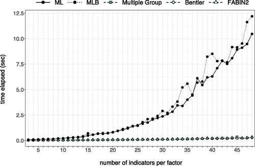
Given their computational simplicity and speed, also the opposite end of the spectrum (big/high-dimensional data) can benefit from non-iterative procedures. Although simulation studies typically include only a limited number of indicators per factor, having hundreds of indicators is no exception in applied research. Consider, for instance, the Big Five personality dimensions as measured by the 240 items in the NEO-Personality Inventory-Revised (Costa & McCrae, 2008). As a proof of concept, we fitted a simple five factor model to NEO-PI R data (Dolan et al., 2009) retrieved from the qgraph package in R (Epskamp et al., 2012, version 1.9.4). Irrespective of the appropriateness of this model (see, for instance, McCrae et al., 1996), this example allows us to demonstrate that estimation time tends to increase as more indicators are included in the model (moving from 3 to 48 indicators per factor). Every model was fitted to the 500 observations with ML, bounded ML (MLB), and three non-iterative procedures as they are currently implemented in lavaan (Rosseel, 2012, version 0.6–16). For a simple model with only three indicators per factor, only small differences were observed between ML (0.087 sec), MLB (0.079 sec), Multiple Group (0.037 sec), Bentler (0.036 sec) and FABIN (0.037 sec). As seen in Figure 1, however, differences between iterative and non-iterative methods grow larger as the measurement models grow. For the full model with 48 indicators per factor, computation times were substantially longer for ML (10.472 sec) and MLB (12.200 sec) compared to Multiple Group (0.312 sec), Bentler (0.281 sec) and FABIN (0.338 sec). Such a computational advantage may prove extremely useful in resampling settings, where computation times quickly accumulate.

Figure 1. Example of increased computation times as the measurement models in a five factor model grow larger. The number of indicators was increased in a stepwise fashion, moving from p = 15 to p = 240 (maximum of 48 indicators per factor).

In this study, we set out to evaluate whether the favorable results of non-iterative methods in confirmatory factor analysis (CFA) generalize to SEMs estimated via SAM. More specifically, we aim to evaluate whether use of non-iterative CFA approaches in the measurement part of the model (step 1) results in accurate parameter estimation of the structural parameters (step 2). Non-iterative methods under consideration are the Multiple Group method (Guttman, 1944, 1952; Holzinger, 1944; Thurstone, 1945), FActor Analysis By INstrumental variables (FABIN, Hägglund, 1982), the non-iterative CFA approach by Bentler (1982), MIIV-2SLS (Bollen, 1989, 2019), and the James-Stein estimator (Burghgraeve et al., 2021). For full details on these estimation procedures, we kindly refer to the original articles. Concise descriptions of the factor-analytic methods are given in the Appendix.

The rest of this article is organized as follows. We first clarify the main differences between standard SEM versus SEM via SAM, introducing the relevant formulae and notation. Then, we discuss the design, methodology and results from our simulation study. We conclude with a discussion of the results and some closing thoughts on perceived opportunities and limitations.

1.2. Traditional SEM

Consider k latent factors measured via p observed variables. A full SEM can be defined by the following pair of equations: (1) $$\mathit{y}=\mathit{\nu }+\mathbf{\Lambda }\mathit{\eta }+\mathit{ϵ}$$(1) (2) $$\mathit{\eta }=\mathit{\alpha }+\mathit{B\eta }+\mathit{\xi }.$$(2)

The first equation formalizes the measurement part of the model, where y is a $p\times 1$ random vector of observed values, $\mathit{\nu }$ is a $p\times 1$ vector of intercepts, $\mathbf{\Lambda }$ is a p × k matrix of factor loadings, $\mathit{\eta }$ is a $k\times 1$ random vector of latent factors, and $\mathit{ϵ}$ is a $p\times 1$ random vector of residuals. The second equation formalizes the structural part of the model, where $\mathit{\alpha }$ is a $k\times 1$ vector of means, B is a k × k matrix of regressions between latent factors with zeros on the diagonal and $(\mathit{I}-\mathit{B})$ invertible, and $\mathit{\xi }$ is a $k\times 1$ random vector of disturbances. We assume that $E(\mathit{ϵ})=E(\mathit{\xi })=\mathbf{0}$ and $\mathit{cov}(\mathit{\eta },\mathit{ϵ})=\mathit{cov}(\mathit{ϵ},\mathit{\xi })=\mathbf{0}.$ From equations (1)(1) $$\mathit{y}=\mathit{\nu }+\mathbf{\Lambda }\mathit{\eta }+\mathit{ϵ}$$(1) and (2)(2) $$\mathit{\eta }=\mathit{\alpha }+\mathit{B\eta }+\mathit{\xi }.$$(2) it follows that the model-implied variance-covariance matrix and mean vector have the following form: (3) $$\mathbf{\Sigma }(\mathit{\theta })=\mathbf{\Lambda }{(\mathit{I-B})}^{\mathbf{-1}}\mathbf{\Psi }{(\mathit{I-B})}^{\mathbf{-1\prime }}{\mathbf{\Lambda }}^{\mathbf{\prime }}+\mathbf{\Theta }$$(3) (4) $$\mathit{\mu }(\mathit{\theta })=\mathit{\nu }+\mathbf{\Lambda }{(\mathit{I-B})}^{\mathbf{-1}}\mathit{\alpha },$$(4) where priming denotes transposition, and $\mathbf{\Theta }$ and $\mathbf{\Psi }$ denote the variance-covariance matrices of $\mathit{ϵ}$ and $\mathit{\xi },$ respectively.

Once the model is hypothesized, its parameter values need to be estimated from the data. Using ML, the values can be found by minimizing the normal theory discrepancy function: (5) $$\begin{array}{cc}{F}_{ML}=ln\hfill & |\mathbf{\Sigma }(\mathit{\theta })|+tr(\mathit{S}\mathbf{\Sigma }{(\mathit{\theta })}^{-1})-ln\left|\mathit{S}\right|-p\hfill \\ \hfill & +{(\overline{\mathit{y}}-\mathit{\mu }(\mathit{\theta }))}^{\prime }\mathbf{\Sigma }{(\mathit{\theta })}^{-1}(\overline{\mathit{y}}-\mathit{\mu }(\mathit{\theta })),\hfill \end{array}$$(5) where $\mathbf{\Sigma }(\mathit{\theta })$ is the model-implied covariance matrix, S is the observed covariance matrix, $\mathit{\mu }(\mathit{\theta })$ is the model-implied mean vector, $\overline{\mathit{y}}$ is the observed mean vector, |.| denotes matrix determinant, and tr(.) denotes the trace operator which takes the sum of the main diagonal elements. The discrepancy function returns a scalar value quantifying the difference between the observed summary statistics (S, $\overline{\mathit{y}}$) and the model-implied summary statistics ($\mathbf{\Sigma }(\mathit{\theta }),\mathit{\mu }(\mathit{\theta })$). The function is non-negative, and zero if there is perfect fit. If there is no mean structure involved, equation (5)(5) $$\begin{array}{cc}{F}_{ML}=ln\hfill & |\mathbf{\Sigma }(\mathit{\theta })|+tr(\mathit{S}\mathbf{\Sigma }{(\mathit{\theta })}^{-1})-ln\left|\mathit{S}\right|-p\hfill \\ \hfill & +{(\overline{\mathit{y}}-\mathit{\mu }(\mathit{\theta }))}^{\prime }\mathbf{\Sigma }{(\mathit{\theta })}^{-1}(\overline{\mathit{y}}-\mathit{\mu }(\mathit{\theta })),\hfill \end{array}$$(5) simplifies to (6) $$F_{ML}=ln|\mathbf{\Sigma }(\mathit{\theta })|+tr(\mathit{S}\mathbf{\Sigma }{(\mathit{\theta })}^{-1})-ln\left|\mathit{S}\right|-p.$$(6)

Minimizing the discrepancy function coincides with finding the parameter values that make the observed data most probable under the assumed model. Note that also other discrepancy functions exist, such as F_ULS, which minimizes the sum of squares of each element in the residual matrix $\mathit{S}-\mathbf{\Sigma }(\mathit{\theta })$ (see, for instance, Schermelleh-Engel et al., 2003). Although less efficient than F_ML, the latter discrepancy function has the advantage that it is consistent without relying on distributional assumptions (Bollen, 1989).

Despite the useful statistical properties of the ML estimator (see, for instance, Bollen, 1989), there are a few well-known issues with the vanilla ML approach. Apart from its vulnerability to structural misspecifications and interpretational confounding (cf. supra), there are at least two additional issues worth mentioning. A first problem relates to how the aforementioned optimization problem is solved. Although it is possible to analytically derive a closed-form solution in some special cases, the optimization problem usually requires the use of iterative root-finding algorithms. Starting with an initial guess of the parameter values, the aim of such algorithms is to repeatedly update the parameter values towards a smaller discrepancy (or, equivalently, a higher likelihood) leveraging first order derivatives (quasi-Newton methods), and possibly second order derivatives (Newton methods) to quickly move towards a (local) minimum (Kochenderfer & Wheeler, 2019). Usually, convergence is said to be reached when (i) there is only a minimal change in estimates (or equivalently, in likelihoods) across two consecutive iterations, (ii) all elements of the gradient are near zero, and (iii) the Hessian is negative definite (in case of maximization) or positive definite (in case of minimization). Especially in smaller samples, there is no guarantee that the algorithm will actually find such a stable minimum (e.g., Boomsma, 1985). Note that optimizing F_ULS instead of F_ML will not circumvent this issue, as optimizing F_ULS proceeds via iterative algorithms as well.

A second issue of ML is that the final estimates may not necessarily be located within the admissible parameter space. Without additional constraints, it is not uncommon to obtain improper solutions, such as negative variances or correlations with an absolute value larger than one (e.g., Anderson & Gerbing, 1984). Although such values may be indicative of flaws in the hypothesized model, this is not necessarily the case. That is, apart from model misspecifications, also sampling fluctuations may give rise to improper values, especially when population values are located close to their boundaries (Van Driel, 1978). As recently shown by De Jonckere and Rosseel (2022), it may be desirable to impose (data-driven) bounds on the parameters, thereby substantially reducing (but not eliminating) both the number of non-convergent and improper solutions.

1.3. SEM via Structural After Measurement

In recent work, Rosseel and Loh (2022) developed a formal framework that builds upon the long-standing idea of separating the structural part of the model from the measurement part (see Burt, 1976; Hunter & Gerbing, 1982; Lance et al., 1988). The authors differentiate between ‘global’ and ‘local’ SAM. Both approaches involve a multi-step procedure where the structural part is estimated after the measurement part.

1.3.1. Step 1: The Measurement Part

In a first step, we estimate ${\mathit{\theta }}_{\mathit{1}}=[\mathit{\nu },\mathbf{\Lambda },\mathbf{\Theta }]$ (i.e., the parameters related to the measurement model). With b denoting the number of measurement blocks, we can choose to fit a separate measurement model to every latent variable (b = k), or to combine multiple latent variables into a single measurement block (b < k). Whereas Rosseel and Loh are generally in favor of using separate measurement blocks to improve robustness against local misspecifications, a joint measurement model may be required when indicators are assumed to be linked (e.g., due to cross-loadings, residual covariances or equality constraints) or indicator reliabilities are very low (e.g., <.50).

Temporarily ignoring the structural part of the model has a few advantageous implications for small sample research. First, a SAM approach can (at least in theory) be useful in very small sample settings, where the number of observations is too small to allow for a classical SEM approach. In order to optimize the normal theory discrepancy function in equation (6)(6) $$F_{ML}=ln|\mathbf{\Sigma }(\mathit{\theta })|+tr(\mathit{S}\mathbf{\Sigma }{(\mathit{\theta })}^{-1})-ln\left|\mathit{S}\right|-p.$$(6) , S needs to be positive definite, which requires that $n\ge p.$ By partitioning the model into separate measurement models, the minimally required sample sizes are automatically less stringent. An arguably more attractive feature of the two-step approach, however, is that it allows for a broader range of possible estimators. That is, while estimates for the measurement models can still be obtained via standard iterative procedures (e.g., optimizing F_ML), also non-iterative estimators from factor-analytic literature can now be employed in step 1. As previously noted, such non-iterative estimators naturally circumvent various small sample issues.

1.3.2. Step 2: The Structural Part

Differences between global and local SAM emerge in the second step, where we obtain estimates for ${\mathit{\theta }}_{\mathit{2}}=[\mathit{\alpha },\mathit{B},\mathbf{\Psi }]$ (i.e., the parameters related to the structural part). In global SAM, the elements from ${\widehat{\mathit{\theta }}}_{\mathit{1}}$ obtained in step 1 are plugged in as fixed parameters in the full SEM in step 2, leaving only the parameters in ${\mathit{\theta }}_{\mathit{2}}$ to be freely estimated. In local SAM (the focus of the current research) the elements from ${\widehat{\mathit{\theta }}}_{\mathit{1}}$ obtained in step 1 are used to estimate the model-implied mean vector and variance-covariance matrix of the latent variables, which can then be used to estimate the structural parameters. From the measurement model in (1(1) $$\mathit{y}=\mathit{\nu }+\mathbf{\Lambda }\mathit{\eta }+\mathit{ϵ}$$(1) ), the authors derive the following expression for $\mathit{\eta }$: (7) $$\begin{array}{cc}\mathit{y}\hspace{0.5em}\hspace{0.17em}\hspace{1em}=& \mathit{\nu }+\mathbf{\Lambda }\mathit{\eta }+\mathit{ϵ}\\ \mathbf{\Lambda }\mathit{\eta }\hspace{1em}=& \mathit{y}-\mathit{\nu }-\mathit{ϵ}\\ \mathit{M}\mathbf{\Lambda }\mathit{\eta }=& \mathit{M}[\mathit{y}-\mathit{\nu }-\mathit{ϵ}]\\ \mathit{\eta }\hspace{0.5em}\hspace{0.17em}\hspace{1em}=& \mathit{M}[\mathit{y}-\mathit{\nu }-\mathit{ϵ}]\end{array}$$(7) where M is a k × p mapping matrix such that $\mathit{M}\mathbf{\Lambda }={\mathit{I}}_{\mathit{k}}.$ Taking the expected value and variance of the final expression, we obtain explicit formulae for $E(\mathit{\eta })$ and $\text{var}(\mathit{\eta })$: (8) $$E(\mathit{\eta })=\mathit{M}[E(\mathit{y})-\mathit{\nu }]$$(8) (9) $$\mathit{var}(\mathit{\eta })=\mathit{M}[\mathit{var}(\mathit{y})-\mathbf{\Theta }]{\mathit{M}}^{\prime }$$(9)

From (8(8) $$E(\mathit{\eta })=\mathit{M}[E(\mathit{y})-\mathit{\nu }]$$(8) ) and (9(9) $$\mathit{var}(\mathit{\eta })=\mathit{M}[\mathit{var}(\mathit{y})-\mathbf{\Theta }]{\mathit{M}}^{\prime }$$(9) ), $\widehat{E(\mathit{\eta })}$ and $\widehat{\mathit{var}(\mathit{\eta })}$ are found by replacing $E(\mathit{y})$ and $\mathit{var}(\mathit{y})$ by their sample counterparts $\overline{\mathit{y}}$ and S, and replacing the remaining parameters by their estimated values $\widehat{\mathit{M}},\widehat{\mathit{\nu }}$ and $\widehat{\mathbf{\Theta }}.$ As $\widehat{\mathit{\nu }}$ and $\widehat{\mathbf{\Theta }}$ have already been estimated in the first step, the only remaining unknown is $\widehat{\mathit{M}}.$ One possible estimator for the mapping matrix M can be derived from the ML discrepancy function in (5(5) $$\begin{array}{cc}{F}_{ML}=ln\hfill & |\mathbf{\Sigma }(\mathit{\theta })|+tr(\mathit{S}\mathbf{\Sigma }{(\mathit{\theta })}^{-1})-ln\left|\mathit{S}\right|-p\hfill \\ \hfill & +{(\overline{\mathit{y}}-\mathit{\mu }(\mathit{\theta }))}^{\prime }\mathbf{\Sigma }{(\mathit{\theta })}^{-1}(\overline{\mathit{y}}-\mathit{\mu }(\mathit{\theta })),\hfill \end{array}$$(5) ), resulting in the following expression: (10) $$\widehat{\mathit{M}}={({\widehat{\mathbf{\Lambda }}}^{\prime }{\widehat{\mathbf{\Theta }}}^{-1}\widehat{\mathbf{\Lambda }})}^{-1}{\widehat{\mathbf{\Lambda }}}^{\prime }{\widehat{\mathbf{\Theta }}}^{-1},$$(10) where all elements on the right hand side are part of ${\widehat{\mathit{\theta }}}_1,$ again already estimated in step 1. Note that this expression may look familiar, as it coincides with Bartlett’s factor score matrix to compute factor scores (Bartlett, 1937, 1938). Interestingly, it can be shown that factor score regression (FSR) with Croon’s correction (Croon, 2002) is a special case of local SAM using the mapping matrix in equation (10)(10) $$\widehat{\mathit{M}}={({\widehat{\mathbf{\Lambda }}}^{\prime }{\widehat{\mathbf{\Theta }}}^{-1}\widehat{\mathbf{\Lambda }})}^{-1}{\widehat{\mathbf{\Lambda }}}^{\prime }{\widehat{\mathbf{\Theta }}}^{-1},$$(10) . This implies that any advantages of FSR also hold for this SAM approach, while avoiding the explicit calculation of factor scores.

Once we have $\widehat{E(\mathit{\eta })}$ and $\widehat{\mathit{var}(\mathit{\eta })},$ there are various ways to estimate the structural parameters. Apart from standard iterative procedures, estimates of ${\mathit{\theta }}_2$ can be obtained non-iteratively as well. When the model is recursive (i.e., when causal effects are strictly unidirectional and disturbances are uncorrelated), the estimation problem reduces to a series of simple linear regressions where explicit formulae yield ${\widehat{\mathit{\theta }}}_2.$ When the model is non-recursive (i.e., when there are feedback loops or correlated disturbances), ${\widehat{\mathit{\theta }}}_2$ can be obtained via two-stage least squares. This implies that iterative procedures can be abandoned at both stages. Bear in mind, however, that a further implication of a two-step approach is that (regardless of the estimator being used) valid standard errors for $\widehat{{\mathit{\theta }}_2}$ will need to take into account the uncertainty that comes from estimating ${\widehat{\mathit{\theta }}}_1$ in step 1. This can be achieved via two-step corrected standard errors (Rosseel & Loh, 2022) or non-parametric resampling procedures.

In what follows, we empirically evaluate the performance of various SEM and SAM approaches across a wide range of settings, assuming that interest lies in the structural part of the model. The focus of our evaluation was twofold: (i) the performance of standard SEM relative to local SAM (irrespective of the estimator used in step 1), and (ii) the performance of local SAM using non-iterative estimators for the measurement part relative to local SAM using iterative procedures for the measurement part.

2. Methods

To cover a wide range of plausible circumstances, two simulation studies were conducted. In both studies, data were generated from a five-factor population model as shown in Figure 2, with each factor being measured by three indicators. A few characteristics were shared across studies: (i) the methods under evaluation, (ii) the outcome measures of interest, (iii) manipulations w.r.t. sample size, and (iv) manipulations w.r.t. the strengths of the structural coefficients. Other manipulations were study-specific: reliability and distribution of indicators (only varied in Study 1), and structural misspecifications and the size of the measurement blocks (only varied in Study 2). An overview of the simulation design can be found in Table 1. More details on each of the manipulations are found below.

Figure 2. Visualization of the five-factor population model. Structural misspecifications occur when factor loadings (dashed single headed arrows) or residual variances (dotted double headed arrows) are present in the population model but not in the analysis model. These misspecifications could either be in the exogenous part of the model (yellow), the endogenous part of the model (green), or both. In addition, also a structural misspecification was considered (blue single headed arrow), omitting the structural path from η_b to η_z in the analysis model, while present in the population model.

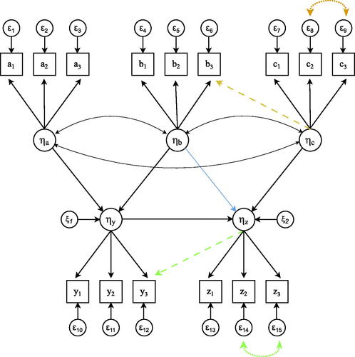
Table 1. Overview of the manipulations in study 1 (reliability, distribution), study 2 (structural misspecifications, number of measurement blocks), as well as the manipulations shared across studies (sample size, strength of regression coefficients expressed in R² value). For study-specific manipulations, asterisks indicate the level at which the variable was held constant in the other study.

Design manipulations
Study 1	Study 2	Across studies
(a) Reliability all high (.80, no spread) all low (.50, no spread)* average low (.50, spread)	(a) Misspecifications no misspecifications${}^{*}$ residual covariances (exo, endo, both) factor loadings (exo, endo, both) structural path (ηb $\to$ ηz)	(a) Sample size
		n = 50
		n = 100
		n = 200
		n = 1000
(b) Distribution normal data${}^{*}$ non-normal data	(b) Measurement blocks single block per factor${}^{*}$ joint for exogenous factors	(b) R squared low (.10) medium (.40)

For every simulated data set out of all 10000 simulations per scenario, the model was estimated via local SAM using the ML mapping matrix and different estimators for the measurement models: bounded ML (SAM-MLB, standard bounds), bounded ULS (SAM-ULSB, standard bounds), Multiple Group method (SAM-MultGroup), FABIN2 ULS (SAM-Fabin2), Bentler ULS (SAM-Bentler), and James-Stein aggregated (SAM-JS). For comparison, the entire model was also fitted as a regular SEM using vanilla ML (SEM-ML), ML using bounds (SEM-MLB), Unweighted Least Squares (SEM-ULS), and Model-Implied Instrumental Variables via Two-Stage Least Squares (SEM-MIIV). Note that methods involving ML, MLB, ULS, or ULSB entail iterative procedures. Every method was evaluated with respect to (i) the number of non-converging solutions, (ii) the number of improper solutions, and (iii) Mean Squared Error (MSE) for the structural parameters. Four different sample sizes were considered (n = 50, n = 100, n = 200, n = 1000), and strengths of the structural coefficients were chosen such that either 10% or 40% of the variability in the outcome variable could be explained by the exogenous variables ($R^2=.10$ or $R^2=.40$).

In Study 1, reliability was varied such that the three indicators per factor could either have reliabilities of .80 (all high), reliabilities of .50 (all low), or average reliabilities of .50 with a spread from .70 to .30 (average low). In case of non-constant reliabilities (average low), highest reliabilities were assigned to the scaling indicators. The distribution of the data was either normal or non-normal, where non-normal data were created by generating factors and residuals with skewness and excess kurtosis values of −2 and 8, respectively.

In Study 2, structural misspecifications were created such that the analysis model would either omit a residual covariance, a factor loading, or the structural path from the analysis model (indicated as dotted double headed, dashed single headed, or dotted single headed arrows in Figure 2). The first two misspecifications could either be located in the exogenous part of the model, the endogenous part of the model, or both. To evaluate the effect of the number of measurement blocks, we either fitted a separate measurement model per latent variable ($b=k=5$) or a joint measurement model for all exogenous variables η_a, η_b and η_c (b = 3).

All simulations were performed in R (R Core Team, 2023) by help of the lavaan (Rosseel, 2012; version 0.6–16) and MIIVsem (Fisher et al., 2021; version 0.5.8) packages. Non-normal data were generated by use of the rIG function from the covsim package (Grønneberg et al., 2022; version 1.0.0). Full R code with all simulation details and population values can be found in our OSF repository via the following link: https://osf.io/f5287/.

3. Results

3.1. Convergence

A visualization of the percentages of non-convergent solutions is found in Figure 3. As anticipated, more convergence failures were observed for smaller sample sizes and weaker structural paths. In Study 1 (varying reliability and distribution), most issues emerged for non-normal data with a large spread in indicator reliability (ranging from .70 to .30 with an average reliability of .50). Despite fitting the exact population model to the data, ML failed in almost 11% of the iterations. Applying bounds effectively resolved convergence issues, as no convergence issues were observed for SEM-MLB. Similarly, no convergence issues emerged when using a (bounded) local SAM approach (SAM-MLB, SAM-ULSB).

Figure 3. Visualization of convergence failures for unbounded iterative methods in study 1 (upper panels) and study 2 (lower panels). Figures only show results for SEM approaches as no convergence issues emerged when using a compartmentalized local SAM approach.

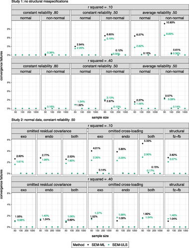
In Study 2 (varying structural misspecifications and number of measurement blocks), omitted cross-loadings had strongest effects on convergence rates, especially in case of small structural effects ($R^2=.10$). Again, bounded approaches (SEM-MLB, SAM-MLB, SAM-ULSB) were able to reach convergence in all iterations, regardless of the number of measurement blocks being used.

3.2. Inadmissible Solutions

Even when a convergent solution was found, it is not necessarily the case that the implied (co)variances can actually exist. Violations against fundamental properties of (co)variances were checked by evaluating the occurrence of negative variances in $\mathbf{\Theta }$ (the covariance matrix of the residual variances) and non-positive definiteness of $\mathbf{\Psi }$ (the covariance matrix of the factors). Violations were determined via the sign of the diagonal elements and the sign of the eigenvalues of the respective matrices. Observed violations for $R^2=.10$ are visualized in Figure 4; similar conclusions are drawn for $R^2=.40.$

Figure 4. Visualization of negative residual variances and non-positive definite latent covariance matrices for iterative methods in study 1 (upper panels) and study 2 (lower panels) where $R^2=.10.$ Figures only show non-zero results for SEM approaches as no issues emerged when using a compartmentalized local SAM approach.

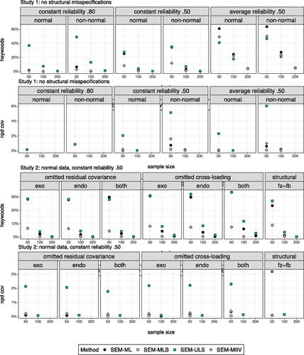
In the least optimal scenario in Study 1 (average low reliability, non-normal data), 63.44% of the solutions for ML contained at least one negative residual variance, and up to 3.34% of the implied latent covariance matrices were not positive definite. As expected, imposing bounds on the parameters successfully avoided the occurrence of Heywood cases. However, also with a bounded SEM-MLB approach, the number of non-positive definite covariance matrices for $\mathit{\eta }$ did not drop entirely to zero. No such inadmissible solutions were observed when adopting a local SAM approach. Also in Study 2 (varying structural misspecifications), only the SAM approaches were entirely free from inadmissible solutions.

3.3. Mean Squared Error

A visual representation of MSE values in Study 1 (varying reliabilities and distributions) is found in Figure 5, where digits show absolute MSE values and colors represent its size relative to SEM-ML. To allow for a fair comparison between SEM-ML and the other methods under evaluation, only data sets for which SEM-ML reached convergence were taken into consideration. As patterns were highly similar across R² values, only results for $R^2=.40$ are reported. Both SEM-ULS and SEM-MIIV show inflated MSE values across all reliabilities and distributions. Imposing bounds on ML successfully improves MSE values, with lower values for SEM-MLB in small samples with low reliabilities. Notably, compartmentalizing the model in separate measurement blocks via a local SAM approaches improves MSE values even further, with lower MSE values for SAM-MLB compared to SEM-MLB. Interestingly, differences between SAM-MLB and other SAM approaches are limited, implying that similar drops in MSE values can be obtained via (less expensive) non-iterative approaches. Note that among non-iterative SAM approaches, SAM-MultGroup and SAM-Bentler tend to outperform SAM-Fabin2 and SAM-JS, with results from the latter two methods being somewhat inconclusive. That is, in the average low reliability condition, these methods occasionally yield slightly inflated (rather than deflated) MSE values.

Figure 5. Overview of MSE values in study 1 (no structural misspecifications, separate measurement block per factor). Cell values show MSE values; cell colors represent its size relative to SEM-ML (i.e., colors moving from white towards blue/orange as they become smaller/larger relative to SEM-ML).

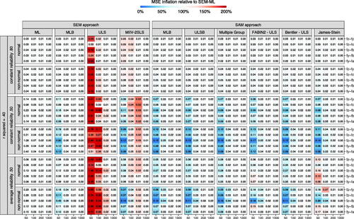
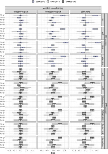
A similar visual representation of MSE values in Study 2 (varying structural misspecifications and the number of measurement blocks) is found in Figure 6. As patterns were highly similar across R² values and the number of measurement blocks, only results for $R^2=.10$ with b = k are reported. General patterns are highly similar to those observed in Study 1. That is, lower MSE values for a compartmentalized approach (SAM-MLB < SEM-MLB) with nearly no differences between SAM-MLB and the non-iterative SAM approaches. Prominent drops in MSE values are observed for the structural path from η_y to η_z in case of an omitted cross-loading in the endogenous part of the model. Note that in contrast to Study 1, drops are observed up to the largest sample size. Closer inspection of biases in point estimates (see Figure 7) shows higher robustness for the local SAM approach. Note that differences between b = k (a separate measurement model per factor) and b < k (a joint measurement model for exogenous variables) were almost negligible.

Figure 6. Overview of MSE values in study 2 (constant reliability of.50, normal data). Cell values show MSE values; cell colors represent its size relative to SEM-ML (i.e., colors moving from white towards blue/orange as they become smaller/larger relative to SEM-ML).

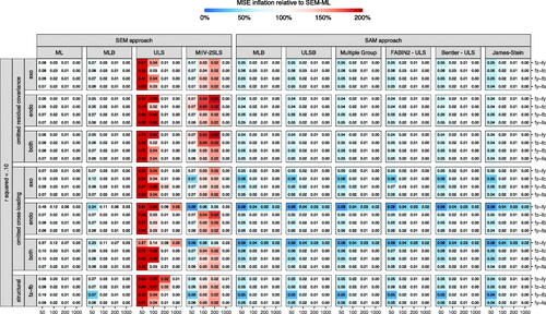
Figure 7. Boxplots of bias in the estimated regression coefficients ($R^2=.40,$n = 1000) in case of an omitted cross-loading in the exogenous part, the endogenous part, or both.

4. Discussion

Previous research has shown that non-iterative procedures are well capable of estimating confirmatory factor analysis models. In this study, we set out to evaluate whether similar conclusions can be drawn for the structural coefficients in a full structural equation model when adopting a local Structural After Measurement (SAM) approach. As SAM proceeds by first estimating the measurement model (step 1) before moving on to the structural model (step 2), it greatly expands the scope of possible estimators, as now also non-iterative methods from factor-analytic literature can be used in the first step of the analysis. Once estimates for the measurement part are obtained (either iteratively or in closed-form), structural coefficients can be estimated via closed-form expressions as well.

Similar to the results from Rosseel and Loh (2022), we found that a local SAM approach outperforms traditional SEM in small to moderate samples (both in terms of convergence and MSE values), especially when reliability drops. Notably, this observation holds regardless of the estimator that is used in step 1, with only small differences between estimators. This implies that the computational simplicity and speed of the closed-form expressions does not compromise their capabilities in terms of parameter recovery. Hence, it seems that the limited interest in these methods has little to do with their performance. Apart from the overall dominance of ML in SEM literature, we presume that the lack of implementation in software is one of the main barriers for using and/or researching these procedures. Therefore, we hope that the implementation in lavaan will pave the way for further research in this area.

With no convergence issues and smaller MSE values, it appears that opting for non-iterative methods over standard ML leaves only one important drawback: stepping outside the ML framework inevitably affects the process of inference. With ML, obtaining standard errors, confidence intervals, and assessing model fit is standard practice with a well-established theoretical foundation. This does not necessarily hold for the non-iterative methods. It should be noted, however, that one simple solution for the fit measures may be to compute so-called ‘pseudo’ fit measures by computing the model-implied summary statistics from the (non-iteratively obtained) point estimates, and then plugging these summary statistics into the ML fit function. From this, we can then obtain a ‘pseudo’ fit statistic. In a similar fashion, we can obtain approximate standard errors by taking the square root of the diagonal elements of a ‘pseudo’ information matrix. These pseudo measures are not (yet) provided in the model output for non-iterative estimators in lavaan, but can be obtained by tricking lavaan into thinking that the estimates were obtained via ML (see Appendix B for example R-code and a comparison between the obtained estimates, SEs, and fit measures). Alternatively, resampling procedures can be used to obtain an empirical estimate of the variability. Whereas performance of a ‘pseudo’ fit measure approach has already been validated in the context of factor score regression (see Devlieger et al., 2019), inference with non-iterative estimators in CFA and SEM via SAM should be addressed in future research.

We conclude that various research settings may benefit from using non-iterative procedures. Whereas ML is likely to remain the go-to method for most well-behaved large sample data, we believe that cheaper non-iterative estimators deserve careful consideration in most real-life applications.

Correction Statement

This article has been corrected with minor changes. These changes do not impact the academic content of the article.

Appendix A.

Non-Iterative Factor-Analytic Methods

Multiple Group

Step 1: Estimate the communality $h_i^2$ for every indicator y_i, for instance by the the method from Spearman (1904) as described in Harman (1976, p. 115): $$h_i^2=\frac{\sum _{j,k=1}^p{s}_{ij}{s}_{ik}}{\sum _{j,k=1}^p{s}_{jk}}$$ where $i\ne j,i\ne k,$ and j < k. Replace the diagonal elements in the variance covariance matrix S by the estimated communalities and denote the resulting matrix ${\mathit{S}}^{\mathit{*}}.$

Step 2: Construct a p × k pattern matrix, X, with binary elements reflecting the hypothesized grouping of indicators. Compute ${\mathit{X}}^{\mathit{\prime }}{\mathit{S}}^{\mathit{*}}$ and denote the resulting product ${\mathit{L}}_{\mathit{0}}.$ This coincides with summing the row elements within ${\mathit{S}}^{\mathit{*}}$ for each group separately. Then, compute ${\mathit{L}}_{\mathit{0}}\mathit{X}$ and denote the resulting product ${\mathit{P}}_{\mathit{0}}.$ This coincides with summing the columns of ${\mathit{L}}_{\mathit{0}}$ for each group separately.

Step 3: Let D denote a diagonal matrix with the same diagonal as ${\mathit{P}}_{\mathit{0}}.$ Compute ${\mathit{L}}_{\mathit{0}}{\mathit{D}}^{\mathit{-1/2}}$ to find the factor structure matrix, L. Compute ${\mathit{D}}^{\mathit{-1/2}}{\mathit{P}}_{\mathit{0}}{\mathit{D}}^{\mathit{-1/2}}$ to find the factor correlation matrix, P. We arrive at the (unconstrained) factor loadings, ${\mathbf{\Lambda }}^{*},$ by multiplying L with the inverse of P. In the general confirmatory case, constrained methods can be used to solve ${\mathbf{\Lambda }}^{*}=\mathit{L}{\mathit{P}}^{\mathit{-1}}.$ In the special case of simple structure and no (in)equality constraints, the computation simplifies to ${\mathbf{\Lambda }}^{*}=\mathit{L}°\mathit{X},$ where $°$ denotes the Hadamard (element-wise) product.

Step 4: Let M denote a k × k diagonal matrix with the loadings of the scaling indicators as its diagonal elements, resulting in a final estimate of $\mathbf{\Lambda }.$ Post-multiplying ${\mathbf{\Lambda }}^{*}$ with the inverse of this matrix ensures that the scaling indicators now have unit loading on their respective factors. A final estimate of $\mathbf{\Psi }$ is obtained by pre- and post-multiplying P by M.

CFA Approach Bentler

Step 1: Group the indicators into two sets: a first set (${\mathit{y}}_{\mathit{1}}$) with k scaling indicators, and a second set (${\mathit{y}}_{\mathit{2}}$) with the remaining $p-k$ indicators. With unit loading on their respective factors, the marker variables are decomposed as ${\mathit{y}}_{\mathit{1}}=\mathit{\eta }+{\mathit{ϵ}}_{\mathit{1}}$ with covariance matrix ${\mathbf{\Sigma }}_{\mathbf{1}\mathbf{1}}=\mathbf{\Psi }+{\mathbf{\Theta }}_{\mathbf{1}}.$ The remaining variables are decomposed as ${\mathit{y}}_{\mathit{2}}={\mathbf{\Lambda }}_{\mathbf{2}}\mathit{\eta }+{\mathit{ϵ}}_{\mathit{2}}$ where ${\mathbf{\Sigma }}_{\mathbf{2}\mathbf{1}}={\mathbf{\Lambda }}_{\mathbf{2}}\mathbf{\Psi }$ and ${\mathbf{\Sigma }}_{\mathbf{2}\mathbf{2}}={\mathbf{\Lambda }}_{\mathbf{2}}\mathbf{\Psi }{\mathbf{\Lambda }}_{\mathbf{2}}{}^{\prime }+{\mathbf{\Theta }}_{\mathbf{2}}.$ Given the expression for ${\mathbf{\Sigma }}_{\mathbf{2}\mathbf{1}},$ rewrite ${\mathbf{\Sigma }}_{\mathbf{2}\mathbf{2}}$ as ${\mathbf{\Sigma }}_{\mathbf{2}\mathbf{2}}={\mathbf{\Sigma }}_{\mathbf{2}\mathbf{1}}{\mathbf{\Psi }}^{-1}{\mathbf{\Sigma }}_{\mathbf{2}\mathbf{1}}{}^{\prime }+{\mathbf{\Theta }}_{\mathbf{2}}.$

Step 2: Estimate ${\mathbf{\Sigma }}_{\mathbf{2}\mathbf{1}}$ via the sample covariance matrix ${\mathit{S}}_{\mathit{21}}$ and plug this estimator into the expression for ${\mathbf{\Sigma }}_{\mathbf{2}\mathbf{2}}.$ Because ${\mathbf{\Sigma }}_{\mathbf{2}\mathbf{2}}={\mathit{S}}_{\mathit{21}}{\mathbf{\Psi }}^{-1}{\mathit{S}}_{\mathit{21}}{}^{\prime }+{\mathbf{\Theta }}_{\mathbf{2}}$ is now a linear rather than a nonlinear function of the remaining unknowns ${\mathbf{\Psi }}^{-1}$ and ${\mathbf{\Theta }}_{\mathbf{2}},$ these parameters can be estimated via unweighted or weighted least squares.

Step 3: Given estimates for ${\mathbf{\Psi }}^{-1}$ and ${\mathbf{\Theta }}_{\mathbf{2}},$ further linear equations yield estimates for the remaining parameters: ${\stackrel{\mathbf{⁁}}{\mathbf{\Theta }}}_{\mathbf{1}}= {\mathit{S}}_{\mathit{11}}-\stackrel{\mathbf{⁁}}{\mathbf{\Psi }}$ and ${\stackrel{\mathbf{⁁}}{\mathbf{\Lambda }}}_{\mathbf{2}}= {\mathit{S}}_{\mathit{21}}{\stackrel{\mathbf{⁁}}{\mathbf{\Psi }}}^{-1}.$ (In)equality constraints can be imposed by use of constrained methods, such as a quadratic program where we specify the constraints under which we want to minimize the function. In the special case of simple structure, computation of ${\stackrel{\mathbf{⁁}}{\mathbf{\Lambda }}}_{\mathbf{2}}$ simplifies to ${\stackrel{\mathbf{⁁}}{\mathbf{\Lambda }}}_{\mathbf{2}}={\mathit{S}}_{\mathit{21}}°\mathit{X}$ where X is a $p-k\times k$ pattern matrix with binary elements reflecting the hypothesized grouping of non-scaling indicators and $°$ denotes the Hadamard (element-wise) product.

FABIN 2

Step 1: Similar to the other FABIN variants, partition the indicators into three sets with k indicators in the first (${\mathit{y}}_{\mathit{1}}$), q indicators in the second (${\mathit{y}}_{\mathit{2}}$), and r indicators in the third (${\mathit{y}}_{\mathit{3}}$). Specifically for FABIN 2, constrain q to 1, such that $r=p-k-1.$

Step 2: For each set of indicators in i = 1, 2, 3, the indicators can be decomposed as ${\mathit{y}}_{\mathit{i}}={\mathbf{\Lambda }}_{\mathbf{i}}\mathit{\eta }+{\mathit{ϵ}}_{\mathit{i}}.$ Because scaling indicators in ${\mathit{y}}_{\mathit{1}}$ are assumed to have unit loadings on their respective factors, we find that $\mathit{\eta }={\mathit{y}}_{\mathit{1}}+{\mathit{ϵ}}_{\mathit{1}}.$ To estimate the loadings for ${\mathit{y}}_{\mathit{2}},$ substitute the expression for $\mathit{\eta }$ in the expression for ${\mathit{y}}_{\mathit{2}}.$ This leads to ${\mathit{y}}_{\mathit{2}}={\mathbf{\Lambda }}_{\mathbf{2}}{\mathit{y}}_{\mathit{1}}+{\mathit{ϵ}}_{\mathit{2}}-{\mathbf{\Lambda }}_{\mathbf{2}}{\mathit{ϵ}}_{\mathit{1}}.$ This expression resembles a conventional linear regression, with the variables in ${\mathit{y}}_{\mathit{1}}$ serving as independent variables and $\widetilde{\mathit{ϵ}}={\mathit{ϵ}}_{\mathit{2}}-{\mathbf{\Lambda }}_{\mathbf{2}}{\mathit{ϵ}}_{\mathit{1}}$ representing a composite error term. Since ${\mathit{y}}_{\mathit{1}}$ is correlated with ${\mathit{ϵ}}_{\mathit{1}},$ however, least squares is no longer suitable for estimating the remaining unknowns because it violates the zero conditional mean assumption. We can, however, use the variables in the third set as instruments, which are correlated with the endogenous variables but uncorrelated with the error term. An instrumental variable estimate FABIN2 can be derived as ${\widehat{\mathit{\lambda }}}_{\mathit{2}}={\mathit{s}}_{\mathit{23}}{\mathit{S}}_{\mathit{31}}{({\mathit{S}}_{\mathit{13}}{\mathit{S}}_{\mathit{31}})}^{-1}.$ The remaining rows in $\mathbf{\Lambda }$ are estimated successively by repeating the procedure for all p variables $k+1,k+2,\dots ,p$ in set 2, each time with all remaining $p-k-1$ variables in set 3. As frequently desired in a confirmatory setting, elements can be constrained to zero by omitting the variables in ${\mathit{y}}_{\mathit{1}}$ that correspond to the factors on which the indicator does not load.

Step 3: Given the estimates for the loadings, estimates for $\mathbf{\Psi }$ and $\mathbf{\Theta }$ are found by minimizing $Q=tr({\mathit{A}}^2)$ with $\mathbf{A}= \mathit{S}-\mathbf{\Lambda }\mathbf{\Psi }\mathbf{\Lambda }\prime -\mathbf{\Theta }$ according to the least squares principle.

Appendix B.

Pseudo Standard Errors and Pseudo Fit Measures

Here, we provide example R code on how to obtain ‘pseudo’ standard errors and ‘pseudo’ fit measures for models estimated via a non-iterative estimator. Although lavaan does not provide these measures by default (yet), one convenient way to obtain them is to trick the software into thinking the estimates were obtained via ML. Note that our example only includes estimates for Multiple Group; an identical approach can be adopted for other non-iterative estimators by simply changing the ‘estimator’ argument in the cfa() function. Additionally, bear in mind that this appendix is only provided as an illustration on how ‘pseudo’ fit measures and standard errors can be obtained. A thorough investigation of the validity of these measures is imperative and should be addressed in future research.

Example R-Code

Table

1 # Load package 2 library("lavaan") 3 4 # Define population model 5 pop.model <- ’ fx =∼ 1*x1 + 0.8*x2 + 0.7*x3 + 0.6*x4 ’ 6 7 # Generate data 8 data <- simulateData(model = pop.model, 9 sample.nobs = 50, 10 seed = 3101997, 11 empirical = FALSE) 12 13 # Define analysis model (no misspecifications) 14 model <- ’ fx =∼ x1 + x2 + x3 + x4 ’ 15 16 # Standard Maximum Likelihood: 17 # Usual approach to obtain estimates, standard errors, fit statistics,… 18 fit <- cfa(model = model, data = data, estimator = "ML") 19 summary(fit) 20 fitMeasures(fit, c("chisq", "df", "pvalue", "cfi", "rmsea")) 21 22 # Multiple Group Method: 23 # A. Trick lavaan into thinking estimates were obtained via ML 24 fit2 <- cfa(model = model, data = data, estimator = "guttman") 25 fit2@Options$estimator <- "ML" 26 fit2@Model@estimator <- "ML" 27 fit2@Options$se <- "standard" 28 29 # B. Compute variance covariance matrix parameters 30 VCOV <- lavaan:::lav_model_vcov(lavmodel = fit2@Model, 31 lavsamplestats = fit2@SampleStats, 32 lavoptions = fit2@Options, 33 lavdata = fit2@Data, 34 lavpartable = fit2@ParTable, 35 lavcache = fit2@Cache, 36 lavimplied = fit2@implied, 37 lavh1 = fit2@h1) 38 39 # C. Compute standard errors 40 fit2@ParTable$se <- lavaan:::lav_model_vcov_se(lavmodel = fit2@Model, 41 lavpartable = fit2@ParTable, 42 VCOV = VCOV) 43 44 # D. Compute fit measures 45 fit2@Options$test <- "standard" 46 fx <- lavaan:::lav_model_objective(lavmodel = fit2@Model, 47 lavsamplestats = fit2@SampleStats, 48 lavdata = fit2@Data) 49 fit2@optim$fx <- fx[1] 50 fit2@optim$fx.group <- attr(fx, "fx.group") 51 52 fit2@test <- lavaan:::lav_model_test(fit2) 53 fitMeasures(fit2, c("chisq", "df", "pvalue", "cfi", "rmsea")) 54 55 # E. Complete fit2 object so we can call summary() 56 fit2@vcov <- list(se = "standard", 57 information = c("expected", "expected"), 58 vcov = VCOV) 59 60 summary(fit2)

Output

The R-code leads us to the following parameter tables for Maximum Likelihood (left) and Multiple Group (right). Note that results are highly similar across methods.

Table

		Maximum Likelihood				Multiple Group
	parameter	est	se	z	pvalue	est	se	z	pvalue
1	fx=∼x1	1.000				1.000
2	fx=∼x2	1.028	0.229	4.484	0.000	1.025	0.220	4.662	0.000
3	fx=∼x3	0.654	0.165	3.963	0.000	0.657	0.161	4.092	0.000
4	fx=∼x4	0.615	0.154	4.009	0.000	0.628	0.149	4.222	0.000
5	x1∼∼x1	0.976	0.281	3.469	0.001	0.988	0.283	3.490	0.000
6	x2∼∼x2	0.796	0.262	3.039	0.002	0.780	0.258	3.025	0.002
7	x3∼∼x3	0.698	0.170	4.112	0.000	0.699	0.171	4.082	0.000
8	x4∼∼x4	0.592	0.145	4.073	0.000	0.563	0.142	3.959	0.000
9	fx∼∼fx	1.168	0.432	2.703	0.007	1.235	0.450	2.747	0.006

Similarly, the pseudo fit measures from Multiple Group lead us to the same conclusions as the fit measures from Maximum Likelihood (i.e., acceptable model fit).

Table

	chisq	df	pvalue	cfi	rmsea
Maximum Likelihood	3.002	2.000	0.223	0.982	0.100
Multiple Group	3.124	2.000	0.210	0.980	0.106

Note that the fit measures from Maximum Likelihood indicate a marginally better fit compared to those from Multiple Group, as suggested by a lower chi-square and RMSEA, and a higher CFI. This outcome was to be expected given that all three fit measures are based on the discrepancy function $F[\mathit{S}-\Sigma (\mathit{\theta })]$ , and the whole idea of ML is that the final estimates minimize this discrepancy function.

References

- Albert, A. A. (1944). The minimum rank of a correlation matrix. Proceedings of the National Academy of Sciences of the United States of America, 30, 144–146. https://doi.org/10.1073/pnas.30.6.144
- Anderson, T. W. (1984). An introduction to multivariate statistical analysis.
- Anderson, J. C., & Gerbing, D. W. (1984). The effect of sampling error on convergence, improper solutions, and goodness-of-fit indices for maximum likelihood confirmatory factor analysis. Psychometrika, 49, 155–173. https://doi.org/10.1007/BF02294170
- Arbuckle, J. (1997). Amos users’ guide. version 3.6.
- Bakk, Z., & Kuha, J. (2018). Two-step estimation of models between latent classes and external variables. Psychometrika, 83, 871–892. https://doi.org/10.1007/s11336-017-9592-7
- Bartlett, M. S. (1937). The statistical conception of mental factors. British Journal of Psychology. General Section, 28, 97–104. https://doi.org/10.1111/j.2044-8295.1937.tb00863.x
- Bartlett, M. S. (1938). Methods of estimating mental factors. Nature, 141, 609–610.
- Bentler, P. M. (1982). Confirmatory factor analysis via noniterative estimation: A fast, inexpensive method. Journal of Marketing Research, 19, 417–424. https://doi.org/10.1177/002224378201900403
- Bentler, P. M. (1985). Theory and implementation of eqs: A structural equations program. BMDP Statistical Software.
- Bollen, K. A. (1989). Structural equations with latent variables. John Wiley & Sons.
- Bollen, K. A. (2019). Model implied instrumental variables (miivs): An alternative orientation to structural equation modeling. Multivariate Behavioral Research, 54, 31–46. https://doi.org/10.1080/00273171.2018.1483224
- Bollen, K. A., Gates, K. M., & Fisher, Z. (2018). Robustness conditions for miiv-2sls when the latent variable or measurement model is structurally misspecified. Structural Equation Modeling : a Multidisciplinary Journal, 25, 848–859. https://doi.org/10.1080/10705511.2018.1456341
- Bollen, K. A., Kirby, J. B., Curran, P. J., Paxton, P. M., & Chen, F. (2007). Latent variable models under misspecification: Two-stage least squares (2sls) and maximum likelihood (ml) estimators. Sociological Methods & Research, 36, 48–86. https://doi.org/10.1177/0049124107301947
- Boomsma, A. (1985). Nonconvergence, improper solutions, and starting values in lisrel maximum likelihood estimation. Psychometrika, 50, 229–242. https://doi.org/10.1007/BF02294248
- Burghgraeve, E. (2021). Alternative estimation procedures for structural equation models. [Unpublished doctoral dissertation]. Ghent University.
- Burghgraeve, E., De Neve, J., & Rosseel, Y. (2021). Estimating structural equation models using james–stein type shrinkage estimators. Psychometrika, 86, 96–130. https://doi.org/10.1007/s11336-021-09749-2
- Burt, R. S. (1973). Confirmatory factor-analytic structures and the theory construction process. Sociological Methods & Research, 2, 131–190. https://doi.org/10.1177/004912417300200201
- Burt, R. S. (1976). Interpretational confounding of unobserved variables in structural equation models. Sociological Methods & Research, 5, 3–52. https://doi.org/10.1177/004912417600500101
- Costa, P., & McCrae, R. R. (2008). The revised neo personality inventory (neo-pi-r). Sage Publications, Inc.
- Croon, M. (2002). Using predicted latent scores in general latent structure models. In G. Marcoulides & I. Moustaki (Eds.), Latent variable and latent structure models (pp. 195–224). Lawrence Erlbaum.
- Cudeck, R. (1991). Noniterative factor analysis estimators, with algorithms for subset and instrumental variable selection. Journal of Educational Statistics, 16, 35–52. https://doi.org/10.3102/10769986016001035
- De Jonckere, J., & Rosseel, Y. (2022). Using bounded estimation to avoid nonconvergence in small sample structural equation modeling. Structural Equation Modeling: A Multidisciplinary Journal, 29, 412–427. https://doi.org/10.1080/10705511.2021.1982716
- Devlieger, I., Talloen, W., & Rosseel, Y. (2019). New developments in factor score regression: Fit indices and a model comparison test. Educational and Psychological Measurement, 79, 1017–1037. https://doi.org/10.1177/0013164419844552
- Dhaene, S., & Rosseel, Y. (2023). An evaluation of non-iterative estimators in confirmatory factor analysis. Structural Equation Modeling: A Multidisciplinary Journal. Advance online publication. https://doi.org/10.1080/10705511.2023.2187285
- Dolan, C. V., Oort, F. J., Stoel, R. D., & Wicherts, J. M. (2009). Testing measurement invariance in the target rotated multigroup exploratory factor model. Structural Equation Modeling: A Multidisciplinary Journal, 16, 295–314. https://doi.org/10.1080/10705510902751416
- Epskamp, S., Cramer, A. O., Waldorp, L. J., Schmittmann, V. D., & Borsboom, D. (2012). qgraph: Network visualizations of relationships in psychometric data. Journal of Statistical Software, 48, 1–18. https://doi.org/10.18637/jss.v048.i04
- Fisher, Z., Bollen, K., Gates, K., Rönkkö, M. (2021). Miivsem: Model implied instrumental variable (miiv) estimation of structural equation models. [Computer software manual]. (R package version 0.5.8). https://CRAN.R-project.org/package=MIIVsem
- Grønneberg, S., Foldnes, N., & Marcoulides, K. M. (2022). covsim: An r package for simulating non-normal data for structural equation models using copulas. Journal of Statistical Software, 102, 1–45. https://doi.org/10.18637/jss.v102.i03
- Guttman, L. (1944). General theory and methods for matric factoring. Psychometrika, 9, 1–16. https://doi.org/10.1007/BF02288709
- Guttman, L. (1952). Multiple group methods for common-factor analysis: Their basis, computation, and interpretation. Psychometrika, 17, 209–222. https://doi.org/10.1007/BF02288783
- Hägglund, G. (1982). Factor analysis by instrumental variables methods. Psychometrika, 47, 209–222. https://doi.org/10.1007/BF02296276
- Harman, H. H. (1976). Modern factor analysis (3rd ed.). University of Chicago press.
- Holzinger, K. J. (1944). A simple method of factor analysis. Psychometrika, 9, 257–262. https://doi.org/10.1007/BF02288737
- Hunter, J. E., & Gerbing, D. W. (1982). Unidimensional measurement, second-order factor analysis, and causal models. Research in Organizational Behavior, 4, 267–320.
- Ihara, M., & Kano, Y. (1986). A new estimator of the uniqueness in factor analysis. Psychometrika, 51, 563–566. https://doi.org/10.1007/BF02295595
- Jöreskog, K. G., & Sörbom, D. (1993). Lisrel 8: Structural equation modeling with the simplis command language. Scientific software international.
- Jöreskog, K. G., Gruvaeus, G. T., & Van Thillo, M. (1970). Acovs a general computer program for analysis of covariance structures. ETS Research Bulletin Series, 1970, i–54. https://doi.org/10.1002/j.2333-8504.1970.tb01009.x
- Kano, Y. (1990). Noniterative estimation and the choice of the number of factors in exploratory factor analysis. Psychometrika, 55, 277–291. https://doi.org/10.1007/BF02295288
- Kaplan, D. (1988). The impact of specification error on the estimation, testing, and improvement of structural equation models. Multivariate Behavioral Research, 23, 69–86. https://doi.org/10.1207/s15327906mbr2301_4
- Kochenderfer, M. J., & Wheeler, T. A. (2019). Algorithms for optimization. Mit Press.
- Kuha, J., & Bakk, Z. (2023). Two-step estimation of latent trait models. arXiv preprint arXiv:2303.16101.
- Lance, C. E., Cornwell, J. M., & Mulaik, S. A. (1988). Limited information parameter estimates for latent or mixed manifest and latent variable models. Multivariate Behavioral Research, 23, 171–187. https://doi.org/10.1207/s15327906mbr2302_3
- Levy, R. (2023). Precluding interpretational confounding in factor analysis with a covariate or outcome via measurement and uncertainty preserving parametric modeling. Structural Equation Modeling: A Multidisciplinary Journal. Advance online publication. https://doi.org/10.1080/10705511.2022.2154214
- McCrae, R. R., Zonderman, A. B., Costa, P. T., Jr, Bond, M. H., & Paunonen, S. V. (1996). Evaluating replicability of factors in the revised neo personality inventory: Confirmatory factor analysis versus procrustes rotation. Journal of Personality and Social Psychology, 70, 552–566. https://doi.org/10.1037/0022-3514.70.3.552
- R Core Team (2023). R: A language and environment for statistical computing [Computer software manual]. Vienna, Austria. https://www.R-project.org/
- Rosseel, Y. (2012). lavaan: An r package for structural equation modeling. Journal of Statistical Software, 48, 1–36. https://doi.org/10.18637/jss.v048.i02
- Rosseel, Y., & Loh, W. W. (2022). A structural after measurement approach to structural equation modeling. Psychological Methods. Advance online publication. https://doi.org/10.1037/met0000503
- Schermelleh-Engel, K., Moosbrugger, H., & Müller, H. (2003). Evaluating the fit of structural equation models: Tests of significance and descriptive goodness-of-fit measures. Methods of Psychological Research Online, 8, 23–74.
- Stuive, I. (2007). A comparison of confirmatory factor analysis methods: Oblique multiple group method versus confirmatory common factor method.
- Thurstone, L. L. (1945). A multiple group method of factoring the correlation matrix. Psychometrika, 10, 73–78. https://doi.org/10.1007/BF02288876
- Van Driel, O. P. (1978). On various causes of improper solutions in maximum likelihood factor analysis. Psychometrika, 43, 225–243. https://doi.org/10.1007/BF02293865