An Alternative Prior for Estimation in High-Dimensional Settings

Abstract

Bayesian estimations of complex regression models with high-dimensional parameter spaces require advanced priors, capable of addressing both sparsity and multicollinearity in the data. The Dirichlet-horseshoe, a new prior distribution that combines and expands on the concepts of the regularized horseshoe and the Dirichlet-Laplace priors, is a novel approach that offers a high degree of flexibility and yields estimates with comparably high accuracy. To evaluate its performance in different frameworks, this study reports on two replicated simulation studies and a real-data example. Across all tested settings, the proposed approach outperforms or achieves similar performance to well-established regularization priors in terms of loss.

Keywords:

• Dirichlet-Laplace parameter space
• prior distribution
• regularized horseshoe
• shrinkage prior
• sparse Bayesian estimation

1. Introduction

Applied research in both natural and social sciences, such as genetics, psychology, and economics, often deals with intricate models using high-dimensional parameter spaces that incorporate several interactions, splines, and quadratic effects (e.g., Brandt et al., 2018; Engle & Rangel, 2008; Watt, 2004). In such settings, estimation techniques such as ordinary least squares tend to provide biased parameter estimates with low accuracy, because asymptotic theories do not hold when the number of predictors D is greater than the number of observations N. When the design matrix is sparse or the data feature high multicollinearity, dimensionality reduction is of particular importance.

To address problems associated with overfitting and overparametrization (Williams & Rodriguez, 2022), frequentist approaches apply penalized regression methods such as L1 or L2 regularization (Marquardt & Snee, 1975; Tibshirani, 1996). In Bayesian frameworks, regularization can be induced through the specification of prior distributions, which allocate substantial probability mass around 0 to shrink small coefficients toward 0. The heavy tails of these distributions create a means to accommodate large coefficients. Renowned examples of such approaches include the spike-and-slab prior (George & McCulloch, 1993; Ishwaran & Rao, 2005; Mitchell & Beauchamp, 1988) and the Bayesian lasso (Park & Casella, 2008). Although these approaches serve as good starting points, various issues emerge, related to their practical use.

Specifically, spike-and-slab priors were considered the gold standard in sparse Bayesian estimation for a long time because of their well-understood theoretical properties and good performance in a variety of settings related to sparsity. However, they become computationally intensive, particularly when used in high-dimensional spaces, because posterior sampling requires a stochastic search over a tremendous space, leading to slow mixing and convergence (Bhadra et al., 2017; Mitchell & Beauchamp, 1988). As noted by Piironen and Vehtari (2017), their results also can be sensitive to prior choices (i.e., slab width and prior inclusion probability), which can be difficult to determine (Ishwaran & Rao, 2005). Moreover, Mitchell and Beauchamp (1988) point out challenges in modeling correlated predictors and class variables with more than two levels.

The popularity of the Bayesian lasso stems largely from its simplicity and computational efficiency (Piironen & Vehtari, 2017). As Park and Casella (2008) note, the Bayesian lasso ensures a unimodal posterior, which facilitates fast convergence and produces meaningful estimates. However, Carvalho et al. (2008) and Armagan et al. (2013) caution that it also insufficiently shrinks small coefficients (representing noise) while overshrinking large coefficients due to its relatively light tails, such that it is less robust to outliers–a notable drawback. Carvalho et al. (2009) also identify two other factors that hamper the performance of the Bayesian lasso method: overestimation of the signal share in the parameter vector and underestimation of the presence of large coefficients. Finally, due to its reliance on a single hyperparameter in the double exponential (Laplace) prior, the Bayesian lasso suffers restricted flexibility and adaptivity to different problems (Brown & Griffin, 2010).

Some more recently developed priors include, for example, continuous shrinkage priors, which sometimes are expressed as one-group global-local scale mixtures of Gaussians, like the horseshoe (Carvalho et al., 2010). These priors achieve good performance in high-dimensional settings with regard to sparsity (Van Der Pas et al., 2014), exhibit adaptivity to unknown sparsity and signal-to-noise ratios (Carvalho et al., 2008), and offer computational efficiency, in the sense that their complexity depends on the sparsity ratio rather than the number of observations (Van Der Pas et al., 2014). Despite its popularity, some shortcomings of the horseshoe limit its practical use. In particular, Piironen and Vehtari (2017) highlight the lack of a possibility to incorporate prior knowledge about the sparsity level in the parameter vector for the global shrinkage hyperparameter. They assert that the default choices encourage solutions in which too many parameters remain unshrunk. Van Der Pas et al. (2014) also report both over- and underestimation of the sparsity ratio when applying full Bayes implementation with a Cauchy prior on the global hyperparameter. Notably, the horseshoe’s shrinkage profile keeps large coefficients unshrunk, which can be a favorable property, but it also can deteriorate performance when the parameters are only weakly identified by the data, such as when dealing with flat likelihoods emerging in logistic regressions with data separation (Piironen & Vehtari, 2017). In addition, it can cause the means of the posteriors to vanish, as observed for the Cauchy prior (Ghosh et al., 2018). Another concern stems from the multimodality of the posterior, caused by correlated predictors, which can raise sampling and convergence issues for the inference algorithms (Piironen & Vehtari, 2017). Noticeable convergence issues have also been reported by Piironen and Vehtari (2015), even for simple regression problems.

More advanced priors include the regularized horseshoe (Piironen & Vehtari, 2017) and Dirichlet-Laplace priors (Bhattacharya et al., 2015). The former is a generalization of the horseshoe and nests the horseshoe as a special case. Accordingly, the regularized horseshoe is commonly applied to high-dimensional regression problems in which the number of predictors is much greater than the number of observations, due to its strong performance in such settings. Furthermore, it can incorporate prior knowledge about the degree of sparsity in the global hyperparameter. By adding a small degree of regularization to the large coefficients, the regularized horseshoe yields more reasonable parameter estimates, ensures that the posterior mean exists, and avoids sampling issues related to divergent transitions (Piironen & Vehtari, 2017). Although these improvements lead to improved performance and applicability of the horseshoe, as Piironen and Vehtari (2017) emphasize, the issues related to multimodality due to correlated predictors still persist. Furthermore, as they demonstrate, a misspecification of the hyperparameters can result in overly strong regularization.

Dirichlet-Laplace priors unify Dirichlet and Laplace priors to induce sparsity in models. Whereas the Laplacian part controls the overall amount of shrinkage, concentrating the Dirichlet elements constrains the number of non-zero coefficients. Thus, Dirichlet-Laplace priors are theoretically sound; they provide a closed-form representation that is appealing theoretically and also allows for an exact representation of the posterior. According to Bhattacharya et al. (2015), Dirichlet-Laplace priors yield efficient posterior computations, with an appropriate chosen concentration rate, such that they offer an optimal posterior concentration (minimax rate of convergence). Nevertheless, their practical use is limited, because the results depend powerfully on the commonly unknown, hard-to-determine concentration parameter, which can exert substantial effects on the results, as demonstrated by Bhattacharya et al. (2015). In Table 1, we provide an overview of the properties of these priors.

2. Article Aims

To overcome some of these limitations, we suggest a novel prior approach, which we call Dirichlet-horseshoe that combines and expands on the principles of the regularized horseshoe and the Dirichlet-Laplace priors. We test its performance by conducting two replicated simulation studies, along with a real-data example. In the first simulation study, which reflects the normal means problem (see Bhattacharya et al., 2015), Gaussian white noise gets added to a high-dimensional vector of signals with varying signal strengths and different sparsity ratios. Then the second simulation study features a multiple regression setting, such that we draw predictor variables from a multivariate normal distribution with varying correlation strengths and generate a sparse vector of regression coefficients from a log-normal distribution. In the real-data example, we replicate the estimation procedure implemented by Fischer et al. (2023) but apply our proposed Dirichlet-horseshoe prior. Fischer et al. (2023) estimate the effects of emotional cues on minute-by-minute, aggregated alcohol consumption in a soccer stadium, on the basis of intensive longitudinal data and by employing a random intercept regime-switching model. The data set consists of 8,820 observations, with 10 predictors at the within-level and 49 predictors at the between-level.

These illustrative studies confirm that the Dirichlet-horseshoe can deal with different sparsity ratios, handle high multicollinearity, and cope well with small N, large D settings. In all setups, its performance, measured in terms of loss, is either superior or similar to that of competing regularization priors. The results suggest that our proposed prior is best suited for sparse, small sample settings (e.g., 100 observations with 5% relevant predictors) that require precise estimates and a high probability of isolating important predictors from less important ones.

3. Common Priors

To distinguish the Dirichlet-horseshoe prior from existing ones, we briefly introduce five well-established approaches, in chronological publication order. More precisely, we introduce three central concepts (“baseline priors”), which are prone to the issues we outlined previously. Then, we present two more recent (“advanced”) priors, on which we build to construct the Dirichlet-horseshoe. Throughout this article, we use N to denote the number of observations, with $i=1,\dots ,N,$ and D to indicate dimensionality, equal to the number of predictor variables in a regression, where $j=1,\dots ,D.$ The vector of regression coefficients to be estimated is signified by $\mathit{\beta },$ and ${\sigma }^2$ represents the noise variance. Vectors and matrices are highlighted in bold.

3.1. Baseline Priors

3.1.1. Spike-and-Slab

The spike-and-slab prior (George & McCulloch, 1993; Ishwaran & Rao, 2005; Mitchell & Beauchamp, 1988) belongs to the class of discrete mixture priors and is based on a binary decision. Either the point mass for β_j is at 0 (i.e., it comes from a spike), or the coefficient is drawn from a diffuse uniform distribution (i.e., it comes from a slab). This prior is often written as a two-component mixture of Gaussian functions (Piironen & Vehtari, 2017) such that $$\begin{array}{c}{\beta }_j|{\lambda }_j,c,\epsilon \sim {\lambda }_j\mathcal{N}\left(0,c^2\right)+\left(1-{\lambda }_j\right)\mathcal{N}\left(0,{\epsilon }^2\right),\\ {\lambda }_j\sim \text{Ber}\left(\pi \right),\end{array}$$ in which the hyperparameter c controls the shape of the distribution (slab width), and π is the prior inclusion probability. This prior establishes an ideal theoretical benchmark, due to its notable properties. First, it fully reflects the concept of regularization, because coefficients can become exactly 0. Second, there exists a closed-form solution for the posterior distribution. By choosing $\epsilon =0$ and replacing the discrete Bernoulli distribution with a continuous Beta, the prior can be expressed as $$\begin{array}{c}{\beta }_j|{\lambda }_j,c\sim {\lambda }_j\mathcal{N}\left(0,c^2\right),\\ {\lambda }_j\sim \text{Beta}\left(\alpha ,\beta \right).\end{array}$$

For example, $\text{Beta}(.5,.5)$ would be an uninformative Jeffrey’s prior.

3.1.2. Bayesian (Adaptive) Lasso

Park and Casella (2008) introduce the Bayesian lasso, $$\pi \left(\mathit{\beta }|{\sigma }^2\right)=\prod _{j=1}^D\frac{\lambda }{2\sqrt{{\sigma }^2}}{e}^{-\lambda \left|{\beta }_j\right|/\sqrt{{\sigma }^2}},$$ for which the shape of the coefficient’s distribution is governed by ${\sigma }^2$ and the fixed shrinkage parameter λ. According to Park and Casella (2008), estimates have both lasso and ridge regression properties, and the posterior mode is equivalent to the frequentist lasso estimator introduced by Tibshirani (1996). In an attempt to allow for different shrinkage for different coefficients, while maintaining parsimony, Leng et al. (2014) propose the Bayesian adaptive lasso, $$\pi \left(\mathit{\beta }|{\sigma }^2\right)=\prod _{j=1}^D\frac{{\lambda }_j}{2\sqrt{{\sigma }^2}}{e}^{-{\lambda }_j\left|{\beta }_j\right|/\sqrt{{\sigma }^2}},$$ which also ensures that the posterior is unimodal, given any choice of λ_j (Leng et al., 2014; Park & Casella, 2008).

3.1.3. Horseshoe

Carvalho et al. (2010) propose the horseshoe, $$\begin{array}{c}{\beta }_j|{\lambda }_j,\tau \sim \mathcal{N}\left(0,{\lambda }_j^2{\tau }^2\right),\\ {\lambda }_j\sim {\mathcal{C}}^{+}\left(0,1\right),\end{array}$$ a prior distribution with a global (τ) and a local (λ_j) shrinkage parameter. The general degree of regularization τ (often referred to as the global regularization component) shrinks all coefficients toward 0; the local regularization component λ_j allows large coefficients to escape shrinkage. The horseshoe’s heavy tails, resulting from the half-Chauchy distribution, allows the prior to accommodate even the largest coefficients.

3.2. Advanced Priors

3.2.1. Dirichlet-Laplace

Dirichlet-Laplace priors (Bhattacharya et al., 2015) are another class of shrinkage priors that extend the global-local approach by introducing relative predictor importance according to a concentration parameter a, as in $$\begin{array}{c}{\beta }_j|{\varphi }_j,\tau \sim \text{DE}\left(0,{\varphi }_j\tau \right),\\ \mathit{\varphi }\sim \text{Dir}\left(a,\dots ,a\right),\\ \tau \sim \text{Gamma}\left(\mathit{\text{Da}},0.5\right).\end{array}$$

The components of the Dirichlet distribution ${\varphi }_j$ add up to 1 (i.e., the Dirichlet is a multivariate generalization of the Beta distribution). In these equations, DE refers to the double exponential (Laplace) distribution. The concentration parameter a guides the sparsity allocation of the probability mass, such that the larger a is, the more mass gets concentrated on one component, and the smaller a is, the sparser the resulting distribution.

3.2.2. Regularized Horseshoe

The regularized horseshoe, as proposed by Piironen and Vehtari (2017), is a generalization of the horseshoe, expressed as: (1) $$\begin{array}{c}{\beta }_j|{\lambda }_j,\tau ,c\sim \mathcal{N}\left(0,{\tau }^2{\tilde{\lambda }}_j^2\right),\\ {\tilde{\lambda }}_j^2=\frac{c^2{\lambda }_j^2}{c^2+{\tau }^2{\lambda }_j^2},\\ {\lambda }_j\sim {\mathcal{C}}^{+}\left(0,1\right).\end{array}$$(1)

If ${\tau }^2{\lambda }_j^2\ll c^2,$ such that β_j is close to 0, then ${\tilde{\lambda }}_j^2\underset{p}{\to }{\lambda }_j^2,$ and Equation (1)(1) $$\begin{array}{c}{\beta }_j|{\lambda }_j,\tau ,c\sim \mathcal{N}\left(0,{\tau }^2{\tilde{\lambda }}_j^2\right),\\ {\tilde{\lambda }}_j^2=\frac{c^2{\lambda }_j^2}{c^2+{\tau }^2{\lambda }_j^2},\\ {\lambda }_j\sim {\mathcal{C}}^{+}\left(0,1\right).\end{array}$$(1) approaches the original horseshoe. But if ${\tau }^2{\lambda }_j^2\gg c^2,$ such that β_j is far from 0, then ${\tilde{\lambda }}_j^2\underset{p}{\to }\frac{c^2}{{\tau }^2},$ and Equation (1)(1) $$\begin{array}{c}{\beta }_j|{\lambda }_j,\tau ,c\sim \mathcal{N}\left(0,{\tau }^2{\tilde{\lambda }}_j^2\right),\\ {\tilde{\lambda }}_j^2=\frac{c^2{\lambda }_j^2}{c^2+{\tau }^2{\lambda }_j^2},\\ {\lambda }_j\sim {\mathcal{C}}^{+}\left(0,1\right).\end{array}$$(1) approaches $\mathcal{N}(0,c^2),$ which is equivalent to the spike-and-slab estimator for the case in which the coefficient comes from a slab. The regularized version enhances the horseshoe in several ways. First, the global shrinkage parameter τ depends on prior information about the sparsity ratio in the design matrix, because $$\begin{array}{c}\tau \sim {\mathcal{C}}^{+}\left(0,{\tau }_0^2\right),\\ {\tau }_0=\frac{p_0}{D-p_0}\frac{\sigma }{\sqrt{N}},\end{array}$$ where p₀ denotes the number of relevant predictor variables. On the basis of the dimensionality of the data set and an assumed number of relevant predictors, the global shrinkage parameter can be defined systematically. Second, sparsity information enters the reformulated local shrinkage parameter ${\tilde{\lambda }}_j$ through τ, which prevents the vanishing mean problem that arises with the horseshoe, as well as the aforementioned issues attributed to weakly identified parameters.

4. The Dirichlet-Horseshoe Prior

To enhance precision and offer more adaptivity, we combine the Dirichlet-Laplace with the regularized horseshoe, such that we integrate the notion of relative levels of predictor importance and local shrinkage, using information on the overall sparsity. The implied hierarchical structure of the Dirichlet-horseshoe then can be expressed as: $$\begin{array}{c}{\beta }_j|{\lambda }_j,{\varphi }_j,\tau ,c\sim \mathcal{N}\left(0,{\tau }^2{\tilde{\lambda }}_j^2{\tilde{\varphi }}_j^2\right),\\ \tau \sim {\mathcal{C}}^{+}\left(0,{\tau }_0^2\right),\\ {\tilde{\lambda }}_j^2=\frac{c^2{\lambda }_j^2}{c^2+{\tau }^2{\lambda }_j^2},\\ \tilde{\mathit{\varphi }}=\mathit{\varphi }D,\\ {\lambda }_j\sim {\mathcal{C}}^{+}(0,\gamma ),\\ \mathit{\varphi }\sim \text{Dir}(a,\dots ,a).\end{array}$$

The proposed Dirichlet-horseshoe unifies global (τ), local (λ_j), and joint ($\mathit{\varphi }$) regularization. The global and local regularization trade off in ${\tilde{\lambda }}_j,$ with the objective of also shrinking large coefficients when they are weakly identified, to prevent flat posteriors. The peculiarity of the Dirichlet distribution maps all components in $\mathit{\varphi }$ between 0 and 1; it guarantees that the sum of these components is equal to 1. Rescaling the components by D allows the Dirichlet-horseshoe to nest the regularized horseshoe estimator as a special case, as long as the posterior for $\tilde{\mathit{\varphi }}=\mathit{1}.$ In practice, this special case is unlikely; it implies equally important predictor variables. However, the Dirichlet-horseshoe might increasingly come to resemble the regularized horseshoe when the predictor variables grow more homogeneous in their explanatory power for the target variable. For $\tilde{\mathit{\varphi }}\ne \mathbf{1},$ the Dirichlet-horseshoe shrinks all predictors that are less important than an average to be stronger than the regularized horseshoe does, such that for ${\tilde{\varphi }}_j<1,$ it holds that ${\tau }^2{\tilde{\lambda }}_j^2{\tilde{\varphi }}_j^2<{\tau }^2{\tilde{\lambda }}_j^2.$ Analogously, any predictor of greater importance than the average is subjected to a smaller degree of shrinkage. In turn, the Dirichlet-horseshoe functions as a regularizer with greater selectivity capacity between important and unimportant signals.

The slab width can be adjusted by means of c. In line with Piironen and Vehtari (2017), we suggest establishing a weakly informative prior for c. A reasonable choice is the inverse-Gamma distribution, $$c^2\sim \text{InvGamma}(\alpha ,\beta ),$$ which has a heavy right and light left tail, so it does not concentrate excessive probability mass near 0, a feature that is desirable for coefficients that already are considered far from 0 (Piironen & Vehtari, 2017). Incorporating global parameters in the model, estimated from available data, also provides a high degree of adaptivity to different sparsity patterns and can control for Type I errors (Berry, 1987; Scott & Berger, 2006). The local regularization component λ_j, drawn from a half-Cauchy distribution, enables our prior to accommodate even the largest coefficients. The component’s impact on the estimator can be controlled by the scale parameter γ. For the optimal choice of τ₀, we follow Piironen and Vehtari (2017) and use: $${\tau }_0=\frac{p_0}{D-p_0}\frac{\sigma }{\sqrt{N}}.$$

Then we define hyperpriors for both the concentration parameter a and the number of relevant predictors p₀ to reduce the dependence of the results on these parameters when little or no prior information is available. To induce sparsity through $\mathit{\varphi },$ the concentration rates must lie between 0 and 1. To increase the degree of sparsity, modelers should choose smaller values. The number of relevant predictors p₀ controls the scale τ₀ of the half-Cauchy distribution from which the global hyperparameter τ is drawn; p₀ is inversely related to the degree of global regularization. In practice, p₀ is often unknown and needs to be sampled. For statistical reasons, we recommend drawing the fraction of relevant predictors η rather than the number of relevant predictors p₀, according to $$p_0=\eta D,$$ because η is a continuous quantity bounded between 0 and 1, which makes it more convenient to sample using numerical methods, such as Markov chain Monte Carlo or Hamiltonian Monte Carlo.

On the basis of empirical experience, Bhattacharya et al. (2015) determine that choosing $a=1/D$ may induce over-shrinkage if some relatively small coefficients exist. They also emphasize that $a=1/D$ can create numerical issues when D is large. In addition to fixing a = 0.5, they use a uniform prior for the concentration rate a, but uniform distributions can lead to slow convergence and high autocorrelation in the chain. Therefore, we recommend drawing a and η from informative Beta distributions, skewed toward 0 (relative to the presumed sparsity ratio), to allocate more prior probability near 0 than near 1. This effort can help the sampler explore the posterior distribution more efficiently. For example, $\text{Beta}(2,8)$ has a mean equal to 0.2, which may be appropriate if the researcher assumes around 20% of the predictors are relevant, a priori. According to our findings, and in an effort to restrain computational expense, it may be reasonable to define one joint parameter ν for both the concentration a and the fraction of relevant predictors η, such that $\eta =a=\nu ,$ with $\nu \sim \text{Beta}(\alpha ,\beta ).$

Figure 1 shows the marginal density of the Dirichlet-horseshoe compared with the other priors. We use the double exponential prior in place of the Bayesian adaptive lasso, because in a Bayesian lasso regression, each regression coefficient follows a conditional double exponential prior (i.e., Laplace prior) (Park & Casella, 2008; Tibshirani, 1996). We observe that the Dirichlet-horseshoe allocates substantial probability mass close to 0 and has a relatively light tail. The tails are large enough to accommodate large coefficients though, and they are more pronounced than those of the double exponential prior. These key features enable the Dirichlet-horseshoe to perform well in relation to the problems of sparse Bayesian regularization and prediction (Polson & Scott, 2010). The density functions provided by horseshoe, regularized horseshoe, and Dirichlet-horseshoe all lack a closed-form representation. We approximate the horseshoe density using the elementary functions, as detailed in Theorem 1 offered by Carvalho et al. (2010). The density functions for the latter two priors are sampled using 10,000,000 draws. We assume N = 100, D = 100, a = 0.5, $\eta =0.5,$ and σ = 1, and we smooth the tails of the regularized and Dirichlet horseshoes by scaling the kernel bandwidth, for illustration.

5. Simulation Studies

We illustrate the finite sample performance of the proposed Dirichlet-horseshoe prior, compared with the other priors, using the normal means problem (Bhattacharya et al., 2015; Van Der Pas et al., 2014), and then a multiple regression problem with correlated predictors under sparsity.

5.1. Simulation Study I: Normal Means Problem

In the normal means problem, we strive to estimate a D-dimensional mean ${\mathit{\theta }}_{\mathit{0}}$ based on a D-dimensional vector of observations y corrupted with Gaussian white noise, $$\begin{array}{c}{y}_j={\theta }_j+{\epsilon }_j,\\ {\epsilon }_j\sim \mathcal{N}(0,1),\end{array}$$ for various sparsity ratios q_D and mean sizes defined by the signal strength A. Particularly, we sample Ω = 100 replicates of a D = 400 dimensional vector y from a ${\mathrm{N}}_D({\mathit{\theta }}_{\mathit{0}},{\mathit{I}}_{\mathit{D}})$ distribution, where ${\mathit{\theta }}_{\mathit{0}}$ has $q_D\in \{0.05,0.1\}$ nonzero entries, all set to a constant value $A\in \{4,5,6\}.$ In turn, we conduct six simulation settings per prior candidate in each replication, for 3,600 simulations in total. Note that $A=\sqrt{2\hspace{0.17em}\mathrm{\text{ln}}\hspace{0.17em}(400)}\approx 3.5$ is the “universal” threshold for this problem (Johnstone & Silverman, 2004; Van Der Pas et al., 2014). Below this threshold, the nonzero components in ${\mathit{\theta }}_{\mathit{0}}$ are too small to be detected (Piironen & Vehtari, 2017). Therefore, we expect the most imprecise estimates to manifest for A = 4.

We also seek to illustrate the impact of the hyperparameter choice ν, which controls both the concentration rate and the fraction of relevant parameters in the Dirichlet-horseshoe prior, by presenting the results for different hyperparameter selections in the simulation study: D = 400, $q_D=0.05,$ and A varying over $A\in \{4,5,6\}.$ The hyperprior choices include $\nu \sim \text{Beta}(2,8),\nu =0.01,\nu =0.1,$ and $\nu =0.5.$

5.2. Simulation Study II: Multiple Regression Problem

In the multiple regression problem, we aim to estimate a D-dimensional parameter vector $\mathit{\beta }$ drawn from a log-normal distribution based on a N × D dimensional design matrix X, which in turn is drawn from a multivariate normal distribution, such that $$\begin{array}{c}{y}_i={\beta }_0+{\beta }_j{x}_{\mathit{\text{ij}}}+{\epsilon }_i,\\ {\beta }_0\sim \mathcal{N}(0,1),\\ \hspace{1em}{\beta }_j\sim \mathcal{L}\mathcal{N}(0,0.5),\\ \mathit{X}\sim {\mathcal{N}}_D(\mathbf{0},\mathbf{\Sigma }),\\ {\epsilon }_i\sim \mathcal{N}(0,1).\end{array}$$

The variance-covariance matrix $\mathbf{\Sigma }$ contains unit standard deviation on its main diagonal and varying, pairwise correlations ρ on its off-diagonals. We set the number of predictors D = 100, let the sample size be $N\in \{80,200\}$ (N < D, N > D), and vary the correlations ρ over $\rho \in \{0.25,0.5,0.75\}$ (weak, moderate, strong). The parameter vector $\mathit{\beta }$ has a sparsity ratio of 20%, such that we set 80 of the 100 predictors to 0. Again, we conduct Ω = 100 replications per setting and prior candidate, which yields a total of 3,600 simulations.

5.3. Estimation

For the estimation, we use the probabilistic programming package PyMC (Salvatier et al., 2016). In particular, we apply the No-U-Turn (NUTS) sampler (Hoffman & Gelman, 2014), a recursive algorithm for continuous variables based on Hamiltonian mechanics. It extends the Hamiltonian Monte Carlo by eliminating the need to set a number of steps, because an automatic stoppage occurs once the sampler starts to make a U-turn. We set a large acceptance probability of 0.99 (the default value is 0.8), which implies a small step size, so that we can achieve non-divergent trajectories for the samples. For each specification, we run three chains with 3,000 iterations and an additional 1,000 burn-in samples that we discard. We monitor convergence with the Gelman-Rubin statistic $\widehat{R}$ (Brooks & Gelman, 1998; Gelman & Rubin, 1992).

6. Results

This section presents the results of both simulation studies. We illustrate the performance of the Dirichlet-horseshoe compared with the alternative priors. Figures 2 and 4 depict the squared error loss corresponding to the posterior median. Tables A1, A2, A3, and A4 in Appendix A present these results in tabular form, along with several additional measures, such as coverage based on the 95% highest density intervals (HDIs), standard deviation of loss, standard deviation of the median, Type I error, $\widehat{R},$ runtime, and number of divergences. These measures are averaged across replications, and all values converge. We present the detailed hierarchical structure of all priors, together with the parameter values used in the simulation studies, in Appendix B.

6.1. Simulation Study I: Normal Means Problem

Figure 2 depicts the loss for varying signal strengths $A\in \{4,5,6\}$ based on sparsity ratios of $q_D=5\%$ (left panel) and $q_D=10\%$ (right panel) for the normal means problem with dimensionality $D=400$. Specifically, for a sparsity ratio of 5% and a signal strength of 4, the lowest loss occurs for the regularized horseshoe (69.3), followed closely by Dirichlet-horseshoe (69.5), Dirichlet-Laplace (70.6), and horseshoe (73.8) priors. Bayesian adaptive lasso and spike-and-slab priors reveal the most imprecise results (97.1 and 96.6), which persists at larger signal strengths too. As the signals strengthen, the losses associated with all priors except spike-and-slab decrease, as is to be expected, because the signal-to-noise ratio grows. For $A=5$ and $A=6$, the Dirichlet-horseshoe achieves the lowest loss (41.8 and 34.0), followed by the horseshoe (43.9 and 34.6) and regularized horseshoe (44.8 and 35.8). The Dirichlet-Laplace prior performance deteriorates (59.9 and 55.8). At a sparsity ratio of 10%, we find similar patterns. For $A=4$, the loss for the Dirichlet-horseshoe (110.0) is slightly higher than that for the Dirichlet-Laplace (108.0) but considerably lower than those of the regularized horseshoe (114.0), horseshoe (118.0), Bayesian adaptive lasso (127.0), and spike-and-slab (137.0). For the signal strengths $A=5$ and $A=6$, the loss of the Dirichlet-horseshoe (81.9 and 66.7) is lowest, and the differences with the other priors grow more pronounced. That is, the horseshoe (89.4 and 73.1) comes second, closely followed by the Dirichlet-Laplace (91.3 and 80.8) and regularized horseshoe (92.6 and 76.7). Overall, the proposed, novel prior consistently demonstrates superior or competitive accuracy on all tested specifications.

Figure 3 illustrates the sensitivity of the Dirichlet-horseshoe to a selection of hyperparameters that constitute the proposed hyperprior $\nu \sim \text{Beta}(2,8)$, together with fixed values of $\nu =0.01$, $\nu =0.1$, and $\nu =0.5$. We evaluate the results on the basis of the loss calculated from the normal means problem with dimensionality $D=400$, sparsity ratio $q_D=5\%$, and varying signal strengths $A\in \{4,5,6\}$. For the smallest signal strength $A=4$, we observe minor differences in losses across the hyperprior choices $\nu \sim \text{Beta}(2,8)$, $\nu =0.1$, and $\nu =0.5$, but the largest loss emerges for $\nu =0.01$. As (Bhattacharya 2015) point out, choosing overly small values for the concentration parameter can lead to overshrinkage and poor performance in the presence of relatively small signals. For $A=5$ and $A=6$, we note the weak sensitivity of the Dirichlet-horseshoe to the hyperprior choice. The differences in loss are rather small, indicating that the choice of hyperparameter has only a minor impact in these settings.

6.2. Simulation Study II: Multiple Regression Problem

Figure 4 depicts the loss estimated from the multiple regression problem with $D=100$ predictors for varying correlation strengths $\rho \in \{0.25,0.5,0.75\}$ (weak, moderate, strong) in samples with $N=80$ observations (left panel) and $N=200$ observations (right panel).

For the small sample size of 80 and weak to moderate predictor correlations, the Dirichlet-horseshoe achieves the lowest loss (1.11 and 1.85), followed by the regularized horseshoe (1.35 and 2.12), horseshoe (1.37 and 2.13), and Dirichlet-Laplace (1.44 and 2.21). Similar to the normal means problem in Simulation Study I, the Bayesian adaptive lasso and spike-and-slab priors produce the most imprecise results, as is true for all the predictor correlations we examine. With strong correlations, the Dirichlet-horseshoe reveals a loss of 4.49–slightly larger than the values for the regularized horseshoe (4.41) and slightly lower than the horseshoe (4.50), and Dirichlet-Laplace (4.66). With a larger sample size (200), our proposed Dirichlet-horseshoe prior exhibits the smallest loss for all predictor correlations $\rho \in \{0.25,0.5,0.75\}$, with values equal to 0.21, 0.33, and 0.76, respectively. Thus, it also achieves the best outcome for strong correlations, followed by regularized horseshoe (0.28, 0.42, 0.90), horseshoe (0.29, 0.43, 0.91), and Dirichlet-Laplace (0.35, 0.51, 1.00).

Generally, the loss of all priors diminishes with the larger sample size but grows with increasing predictor correlations, which is reasonable, in that it becomes more challenging for the algorithms to disentangle predictor variables. As in the normal means problem, our proposed Dirichlet-horseshoe prior achieves superior or highly competitive accuracy for all the tested specifications.

7. Real-Data Example: Alcohol Use and Emotional Cues

In this section, we extend the performance illustration with a real-data example. Similar to Fischer et al. (2023), we estimate the effect of the reference point-dependent emotional cues Surprise and Suspense (Ely et al., 2015), with the same data set and using their proposed hierarchical state-switching model. However, we apply the Dirichlet-horseshoe instead of the spike-and-slab prior used by those authors. The data set consists of minute-by-minute recorded beer sales in a soccer stadium, as well as data related to in-play betting odds, in-play match events, and match-day information. The design matrix contains 10 predictors at the within-level and 49 predictors at the between-level. All data are observed over six soccer seasons, from 2013/14 to 2018/19, which entail 98 matches, leading to $98\times 90=8,820$ observations in total (a match lasts 90 minutes). Away-team stands are excluded from this sample.

Fischer et al. (2023) follow Buraimo et al. (2020) and use betting odds to estimate outcome probabilities p for all potential outcomes of the match, namely, home win (H), draw (D), or away win (A), in each match minute t. Using these estimated probabilities, they calculate the constructs Surprise and Suspense. Fischer et al. (2023) also determine (emotional) states S = 0 and S = 1 on basis of these estimates, such that Surprise, calculated as, $${\mathit{\text{Surprise}}}_t=u\left(\sum _{m\in H,D,A}{\left[p_t^m-p_{t-1}^m\right]}^2\right),$$ is high if the current outcome probabilities contradict the anterior beliefs (backward-looking). In contrast, Suspense, $${\mathit{\text{Suspense}}}_t= u[\sum _{m\in H,D,A}{p}_{t+1}^{\mathit{\text{HG}}}{\{(p_{t+1}^m|p_{t+1}^{\mathit{\text{HG}}})-p_t^m\}}^2+p_{t+1}^{\mathit{\text{AG}}}{\{(p_{t+1}^m|p_{t+1}^{\mathit{\text{AG}}})-p_t^m\}}^2],$$ is a forward-looking measure that increases when the variance related to possible outcomes in the next minute is high. Here, $p_{t+1}^{\mathit{\text{HG}}}$ is the probability that the home team scores in the next minute. The superscript “AG” instead refers to the away team’s probability of scoring. The utility function is $u(·)=\sqrt{·}$ for both measures. The two emotional states then are given as $$\begin{array}{cc}{p}_t^H\hfill & <p_{t-1}^H\hspace{1em}\Rightarrow \hspace{1em}S=0,\text{and}\\ p_t^H\hfill & >p_{t-1}^H\hspace{1em}\Rightarrow \hspace{1em}S=1,\hfill \end{array}$$ where S = 0 denotes the negative state, because the outcome probabilities for the home team have decreased from the last period to the current period. The positive state is indicated by S = 1. These states are well-justified, because consumption by home and away team fans is separated by stands. This model also allows for a random intercept at the between-level. The within-level is given by, $$\begin{array}{cc}[\mathrm{\text{ln}}\hspace{0.17em}(Y_{1\mathit{\text{it}}})|S_{\mathit{\text{it}}}=s]={\nu }_{1i}\hfill & +\sum _{\text{l = 1}}^L\hspace{0.17em}\mathrm{\text{ln}}\hspace{0.17em}(Y_{1i(t-l)}){\varphi }_{1\mathit{\text{sl}}}\hfill \\ \hfill & +\sum _{l=0}^L({\mathit{X}}_{\mathit{1i}(\mathit{t}-\mathit{l})}{\mathit{\beta }}_{\mathit{1}\mathit{\text{sl}}}+{\mathit{Z}}_{\mathit{1i}(\mathit{t}-\mathit{l})}{\mathit{\gamma }}_{\mathit{1}\mathit{\text{sl}}})\hfill \\ \hfill & +{\psi }_{1\mathit{\text{ts}}}+{\epsilon }_{1\mathit{\text{it}}},\hfill \end{array}$$ where, $${\nu }_{1i}={\mathit{Z}}_{\mathit{2i}}{\mathit{\gamma }}_{\mathit{2}}+{\upsilon }_{2i},$$ at the between-level. Beer sales are collected in Y, and ${\mathit{X}}_{\mathit{1i}(\mathit{t}-\mathit{l})}$ contains the key regressors, Surprise and Suspense. Covariates in ${\mathit{Z}}_{\mathit{1i}(\mathit{t}-\mathit{l})},$ capturing weather conditions and match key events, among other variables, control for potential confounds at the within-level. Covariates related to match-specific information, like the number of spectators, beer price, weekday, and so on, and gathered by ${\mathit{Z}}_{\mathit{2i}},$ control for confounds at the between-level. We use the estimation procedure described for Simulation Studies I and II. Figure 5 presents the results based on Dirichlet-horseshoe. The regressors are standardized, and the dependent variable contains inverse hyperbolic sine-transformed sales. Therefore, the marginal effects can be interpreted in terms of a one standard deviation increase. Our results resonate with the main findings of Fischer et al. (2023). We find predominantly positive effects for Surprise and negative effects for Suspense on the number of beer sales in both states. Moreover, the effects are stronger for the positive state S = 1 overall. We observe a greater level of decisiveness (sharpness) for the Dirichlet-horseshoe compared with the spike-and-slab prior when it comes to variable selection. Accordingly, we observe a higher density allocated around 0 for small-coefficient posteriors exposed at lags 6-8, for example, as well as slightly weaker effects for Suspense when l = 3. For some nonzero posteriors, the probability mass locally peaks close to 0 though. The resulting tendency for multimodal posteriors is typical of horseshoe priors, due to the global and local shrinkage aspects.

8. Discussion

We present the Dirichlet-horseshoe, a novel prior designed for sparse estimations in high-dimensional settings, which integrates the concept of Dirichlet-Laplace priors with the regularized horseshoe. In two simulation studies and a real-data example, we demonstrate that the proposed prior yields more accurate estimates than both well-established and recently developed methods, namely, the spike-and-slab prior, Bayesian adaptive lasso, horseshoe, Dirichlet-Laplace, and regularized horseshoe. Our approach offers a reliable default choice for addressing problems related to varied levels of sparsity (i.e., identifying needles and straws in haystacks), and it exhibits favorable convergence properties. Considering the normal means problem with sparsity ratios of 5% and 10%, our proposed prior achieves significantly better performance than the spike-and-slab and Bayesian adaptive lasso; it performs similarly to the horseshoe, Dirichlet-Laplace, and regularized horseshoe priors at a signal strength of 4. At higher signal strengths (5 or 6), the proposed Dirichlet-horseshoe exhibits a slight advantage over all these priors, showcasing its superior performance.

The Dirichlet-horseshoe also is well suited for small N, large D problems, and it can deal with correlated predictor variables. Specifically, for weak to moderate correlations (i.e., 0.25 to 0.5), the Dirichlet-horseshoe provides more accurate estimates than competing priors. Furthermore, even in the presence of strong correlations, the prior continues to be more accurate, as long as the sample sizes are sufficiently large. Our novel prior further offers a significant degree of flexibility, allowing for easy customization to accommodate specific settings, as demonstrated in the real-data example. Therefore, we consider the Dirichlet-horseshoe prior relevant for a wide range of application fields. It also can address various common challenges in modern statistics, including high-parametric, complex settings, such as network models (Epskamp et al., 2017) or dynamic latent variable models (Kelava & Brandt, 2019), as well as common regression and classification tasks, function estimation, and covariance matrix regularization.

Unless substantial knowledge about the hyperpriors of the Dirichlet-horseshoe exists, we advocate for using the parameters in Equation (B1)(B1) $$\begin{array}{c}{\beta }_j|{\lambda }_j,{\psi }_j,\tau ,c\sim \mathcal{N}\left(0,{\tau }^2{\tilde{\lambda }}_j^2{\tilde{\varphi }}_j^2\right)\\ \tau \sim {\mathcal{C}}^{+}\left(0,{\tau }_0^2\right)\\ {\tilde{\lambda }}_j^2=\frac{c^2{\lambda }_j^2}{c^2+{\tau }^2{\lambda }_j^2}\\ \tilde{\mathit{\varphi }}=\mathit{\varphi }D\\ {\lambda }_j\sim {\mathcal{C}}^{+}\left(0,1\right)\\ \mathit{\varphi }\sim \text{Dir}(\nu ,\dots ,\nu )\\ c^2\sim \text{InvGamma}\left(1,4\right)\\ {\tau }_0=\frac{p_0}{D-p_0}\frac{\sigma }{\sqrt{N}}\\ p_0=\nu D\\ \nu \sim \text{Beta}(2,8)\end{array}$$(B1) as a good starting point. Furthermore, we emphasize that this novel approach extends beyond this particular option; it may be possible to test alternative hyperpriors as well. We use full Bayesian inference for the hyperpriors since opting for empirical Bayes estimation of hyperparameters (as highlighted in the advantages of the empirical Bayes method by Petrone et al. (2014)) or using cross-validation would pose computational difficulties and would not allow accounting for the characteristics of the posterior distributions. When using numerical methods for posterior estimation, such as Markov chain Monte Carlo, Hamiltonian Monte Carlo, or NUTS, we recommend a noncentered representation of the densities, combined with small step sizes, to achieve fewer divergences in the trajectories for the samples. Continued research might investigate reducing the computational expense required for Dirichlet-horseshoe, without sacrificing its performance. Tests of the prior in various applications also are required to confirm its robustness and further specify both its strengths and its weaknesses.

Disclosure Statement

No potential conflict of interest was reported by the authors.

Data Availability Statement

The data and code that support the findings of this study are openly available at https://zenodo.org/doi/10.5281/zenodo.10707994.

Additional information

Funding

This work was funded by the Deutsche Forschungsgemeinschaft (DFG, German Research Foundation) under Germany’s Excellence Strategy - EXC number 2064/1 - Project number 390727645.

Appendix A.

Further results

Figure 1. Marginal density of the Dirichlet-horseshoe (DHS) in comparison with those of the double exponential (DE), horseshoe (HS), Dirichlet-Laplace (DL), and regularized horseshoe (RHS) priors.

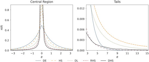
Figure 2. Squared error loss corresponding to the posterior median derived from the normal means problem (Simulation Study I), with a D = 400 dimensional parameter vector for varying signal strengths $A\in \{4,5,6\}$ and sparsity ratios $q_D=5\%$ (left panel) and $q_D=10\%$ (right panel). We abbreviate the considered priors SPSL (spike-and-slab), BAL (Bayesian Adaptive lasso), HS (horseshoe), DL (Dirichlet-Laplace), RHS (regularized horseshoe), and DHS (Dirichlet-horseshoe).

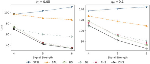
Figure 3. Squared error loss corresponding to the posterior median for different hyperparameter choices ν, derived from the normal means problem with a D = 400 dimensional parameter vector, sparsity ratio $q_D=5\%,$ and varying signal strengths $A\in \{4,5,6\}.$

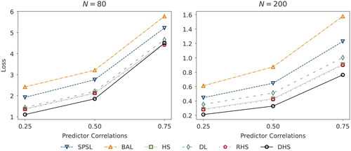
Figure 4. Squared error loss corresponding to the posterior median derived from the multiple regression setting (Simulation Study II) with a D = 100 dimensional parameter vector drawn from a log-normal distribution for varying correlations $\rho \in \{0.25,0.5,0.75\}$ and observations N = 80 (left panel) and N = 200 (right panel). The design matrix is generated by a multivariate normal distribution with correlated predictors. The parameter vector $\mathit{\beta }$ has a sparsity ratio of 20%, such that we set 80 of the 100 predictors to 0. We abbreviate the priors SPSL (spike-and-slab), BAL (Bayesian Adaptive lasso), HS (horseshoe), DL (Dirichlet-Laplace), RHS (regularized horseshoe), and DHS (Dirichlet-horseshoe).

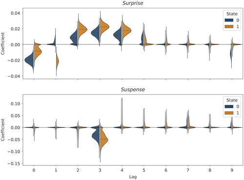
Figure 5. Posterior distributions of the effects of the emotional cues Surprise and Suspense on beer sales, derived from the real-data example. The figure shows posteriors for all lags in both states (negative S = 0 and positive S = 1). The dotted lines indicate the estimated median effect.

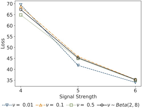
Table 1. This table provides a brief summary of the properties of prior distributions.

Spike-and-Slab	Bayesian (Adaptive) Lasso
discrete (point-mass mixture) prior; continuous versions exist	continuous shrinkage prior
good performance in most settings, in terms of sparsity	simple and fast computations
well-understood theoretical properties	ensures unimodal posteriors
computationally intensive in high-dimensional spaces	limited flexibility and adaptivity
results sensitive to hyperprior choices difficulties in modeling correlated predictors difficulties in modeling class variables with more than two levels	undershrinkage of noise and overshrinkage of large coefficients overestimation of signal density
Horseshoe	Dirichlet-Laplace
continuous shrinkage prior	continuous shrinkage prior
good performance in high-dimensional, sparse settings	existing closed-form representation
adaptivity to unknown sparsity and signal-to-noise ratio	efficient posterior computation
complexity not dependent on number of observations	optimal posterior concentration
no possibility of including prior knowledge of sparsity ratios over- and underestimation of sparsity ratio large coefficients left unshrunk correlated predictors can cause multimodal posteriors convergence and sampling issues	results strongly dependent on unknown concentration parameter
Regularized Horseshoe
continuous shrinkage prior	generalization of the horseshoe that nests it
good performance in high-dimensional settings improved sampling robustness results sensitive to hyperparameter choices	ability to include prior knowledge about the degree of sparsity correlated predictors can cause multimodal posteriors

Table A1. This table presents performance metrics based on 95% HDIs, averaged across simulation replicates. The measures are derived from the normal means problem (Simulation Study I) with a D = 400 dimensional parameter vector. We perform Ω = 100 replications for all combinations of signals strengths $A\in \{4,5,6\}$ and sparsity ratios $q_D\in \{0.05,0.1\}.$ We consider the spike-and-slab (SPSL), Bayesian Adaptive lasso (BAL), horseshoe (HS), Dirichlet-Laplace (DL), regularized horseshoe (RHS), and Dirichlet-horseshoe (DHS) priors.

		Loss	StdLoss	StdMedian	Coverage	Loss	StdLoss	StdMedian	Coverage
A = 4	SPSL	96.6	0.1431	0.6510	0.9812	137.0	0.1348	0.7284	0.9747
	BAL	97.1	0.1689	0.7146	0.9923	127.0	0.1496	0.7334	0.9857
	HS	73.8	0.2784	0.4539	0.9892	118.0	0.1957	0.5862	0.9815
	DL	70.6	0.2244	0.6309	0.9919	108.0	0.1840	0.6546	0.9845
	RHS	69.3	0.2673	0.5014	0.9889	114.0	0.1822	0.6330	0.9814
	DHS	69.5	0.2939	0.4494	0.9900	110.0	0.2057	0.5875	0.9826
A = 5	SPSL	102.0	0.1411	0.6951	0.9852	141.0	0.1273	0.7587	0.9859
	BAL	90.0	0.1739	0.7137	0.9955	117.0	0.1581	0.7310	0.9913
	HS	43.9	0.3480	0.4728	0.9935	89.4	0.2312	0.5997	0.9889
	DL	59.9	0.2387	0.6292	0.9956	91.3	0.2032	0.6510	0.9909
	RHS	44.8	0.3369	0.5020	0.9931	92.6	0.2126	0.6310	0.9905
	DHS	41.8	0.3582	0.4535	0.9938	81.9	0.2471	0.5772	0.9893
A = 6	SPSL	110.0	0.1436	0.7243	0.9878	144.0	0.1187	0.7788	0.9871
	BAL	86.8	0.1711	0.7128	0.9957	109.0	0.1431	0.7295	0.9922
	HS	34.6	0.3198	0.4743	0.9971	73.1	0.1925	0.6025	0.9927
	DL	55.8	0.2292	0.6277	0.9962	80.8	0.1732	0.6490	0.9922
	RHS	35.8	0.3181	0.4934	0.9968	76.7	0.1892	0.6239	0.9925
	DHS	34.0	0.3303	0.4470	0.9971	66.7	0.2099	0.5653	0.9931

Table A2. See the descriptive notes to Table A1.

		TypeIErr	Rhat	Minutes	Divergences	TypeIErr	Rhat	Minutes	Divergences
A = 4	SPSL	0.0004	1.00	0.4216	0	0.0012	1	0.4864	0
	BAL	0.0012	1.00	2.00	21	0.0015	1.00	1.90	31
	HS	0.0001	1.00	0.9389	118	0.0002	1.00	1.11	105
	DL	0.0005	1.00	2.54	0	0.0005	1.00	2.42	0
	RHS	0.0001	1.00	0.4583	0	0.0005	1	0.4244	0
	DHS	0.0001	1.00	4.68	7.49	0.0003	1.00	4.29	3.38
A = 5	SPSL	0.0009	1.00	0.5204	0	0.0017	1	0.4934	0
	BAL	0.0014	1.00	1.97	25.4	0.0012	1.00	1.88	30.9
	HS	0.0001	1.00	0.9861	131	0.0003	1.00	1.34	95
	DL	0.0006	1.00	2.40	0	0.0006	1.00	2.42	0
	RHS	0.0001	1.00	0.4315	0.0400	0.0005	1	0.4438	0
	DHS	0.0002	1.01	4.47	4.60	0.0003	1.00	4.44	1.83
A = 6	SPSL	0.0014	1.00	0.4924	0	0.0024	1	0.5030	0
	BAL	0.0014	1.00	1.89	23	0.0013	1.00	1.88	31.8
	HS	0.0001	1.00	1.09	116	0.0003	1.00	1.36	109
	DL	0.0005	1.00	2.42	0	0.0005	1.00	2.41	0
	RHS	0.0002	1.00	0.4359	0	0.0005	1	0.4540	0
	DHS	0.0001	1.00	4.45	1.40	0.0003	1.00	4.47	1.25

Table A3. This table presents performance metrics based on 95% HDIs, averaged across simulation replicates. The measures are derived from the multiple regression setting (Simulation Study II) with a D = 100 dimensional parameter vector drawn from a log-normal distribution. The design matrix is generated by a multivariate normal distribution with correlated predictors. We perform Ω = 100 replications for all combinations of observations $N\in \{80,200\}$ and correlations $\rho \in \{0.25,0.5,0.75\}.$ We consider the spike-and-slab (SPSL), Bayesian Adaptive lasso (BAL), horseshoe (HS), Dirichlet-Laplace (DL), regularized horseshoe (RHS), and Dirichlet-horseshoe (DHS) priors.

		Loss	StdLoss	StdMedian	Coverage	Loss	StdLoss	StdMedian	Coverage
\rho = 0.25	SPSL	1.92	0.4223	0.2256	0.9948	0.4456	0.2645	0.0869	0.9885
	BAL	2.42	0.4099	0.2744	0.9972	0.6116	0.2233	0.0946	0.9841
	HS	1.37	0.4449	0.1579	0.9878	0.2860	0.3186	0.0721	0.9884
	DL	1.44	0.4377	0.1917	0.9939	0.3525	0.2883	0.0804	0.9898
	RHS	1.35	0.4422	0.1586	0.9884	0.2791	0.3235	0.0715	0.9879
	DHS	1.11	0.5348	0.1280	0.9868	0.2121	0.3872	0.0594	0.9881
\rho = 0.50	SPSL	2.76	0.3267	0.2600	0.9946	0.6471	0.2536	0.1057	0.9898
	BAL	3.21	0.2827	0.3114	0.9981	0.8737	0.2278	0.1144	0.9870
	HS	2.13	0.3693	0.1903	0.9864	0.4316	0.2859	0.0879	0.9887
	DL	2.21	0.3544	0.2291	0.9939	0.5116	0.2752	0.0977	0.9907
	RHS	2.12	0.3599	0.1944	0.9868	0.4198	0.2910	0.0868	0.9885
	DHS	1.85	0.4337	0.1624	0.9850	0.3291	0.3506	0.0741	0.9888
\rho = 0.75	SPSL	5.22	0.3433	0.3254	0.9904	1.23	0.2698	0.1467	0.9885
	BAL	5.77	0.3284	0.3875	0.9954	1.58	0.2455	0.1574	0.9866
	HS	4.50	0.3840	0.2512	0.9805	0.9078	0.2818	0.1221	0.9860
	DL	4.66	0.4054	0.3030	0.9903	1.00	0.2915	0.1356	0.9884
	RHS	4.41	0.3748	0.2590	0.9826	0.8957	0.2844	0.1216	0.9856
	DHS	4.49	0.4476	0.2254	0.9768	0.7623	0.3345	0.1064	0.9857

Table A4. See the descriptions for Table A3.

		TypeIErr	Rhat	Minutes	Divergences	TypeIErr	Rhat	Minutes	Divergences
\rho = 0.25	SPSL	0.0000	1.00	0.3974	0	0.0025	1.00	0.5614	0
	BAL	0.0000	1.00	0.8220	120	0.0076	1.00	0.9750	94.5
	HS	0.0003	1.00	0.7104	64.9	0.0005	1.00	0.9305	76.8
	DL	0.0001	1.00	0.9277	0.3800	0.0014	1.00	1.06	2.99
	RHS	0.0003	1.00	0.5096	0.1500	0.0005	1.01	0.6999	0.4700
	DHS	0.0003	1.00	1.58	11	0.0003	1.01	1.66	24.7
\rho = 0.50	SPSL	0.0004	1.00	0.5328	0	0.0022	1.00	0.6584	0
	BAL	0.0001	1.00	0.8209	82.4	0.0063	1.00	0.9727	79.8
	HS	0.0003	1.00	0.7402	69.1	0.0006	1.00	0.9357	58.6
	DL	0.0001	1.00	0.9274	1.17	0.0011	1.00	1.06	6.06
	RHS	0.0003	1.01	0.5613	0.0700	0.0005	1.00	0.9318	0.3900
	DHS	0.0001	1.00	1.58	13.4	0.0003	1.00	1.66	23
\rho = 0.75	SPSL	0.0006	1.00	0.6019	0	0.0022	1.00	0.8126	0
	BAL	0.0004	1.00	0.8207	68.8	0.0046	1.00	0.9755	88
	HS	0.0006	1.00	0.7695	71.2	0.0004	1.00	0.9376	79.6
	DL	0.0006	1.00	0.9262	1.36	0.0013	1.00	1.06	6.39
	RHS	0.0009	1.00	0.6668	0.0400	0.0006	1.00	1.07	0.1300
	DHS	0.0009	1.00	1.58	10.5	0.0004	1.00	1.66	16.3

Appendix B. Priors simulation studies

B.1 Spike-and-slab

$$\begin{array}{c}{\beta }_j|{\lambda }_j,c,\sim {\lambda }_j\mathcal{N}\left(0,c^2\right)\\ {\lambda }_j\sim \text{Beta}\left(.5,.5\right)\\ c^2\sim \text{InvGamma}(1,4)\end{array}$$

B.2 Bayesian Adaptive Lasso

$$\begin{array}{c}{\beta }_j|{\lambda }_j,\sim \text{DE}\left(0,\frac{1}{{\lambda }_j}\right)\\ {\lambda }_j,\sim {\mathcal{C}}^{+}\left(0,1\right)\end{array}$$

B.3 Horseshoe

$$\begin{array}{c}{\beta }_j|{\lambda }_j,\tau \sim \mathcal{N}\left(0,{\lambda }_j^2{\tau }^2\right)\\ {\lambda }_j\sim {\mathcal{C}}^{+}\left(0,1\right)\\ \tau \sim {\mathcal{C}}^{+}\left(0,1\right)\end{array}$$

B.4 Dirichlet-Laplace

$$\begin{array}{c}{\beta }_j|{\varphi }_j,\tau \sim \text{DE}\left(0,{\varphi }_j\tau \right)\\ \mathit{\varphi }\sim \text{Dir}\left(.5,\dots ,.5\right)\\ \tau \sim \text{Gamma}\left(\frac{D}{2},\frac{1}{2}\right)\end{array}$$

B.5 Regularized Horseshoe

$$\begin{array}{c}{\beta }_j|{\lambda }_j,\tau ,c\sim \mathcal{N}\left(0,{\tau }^2{\tilde{\lambda }}_j^2\right)\\ \tau \sim {\mathcal{C}}^{+}\left(0,{\tau }_0^2\right)\\ {\tilde{\lambda }}_j^2=\frac{c^2{\lambda }_j^2}{c^2+{\tau }^2{\lambda }_j^2}\\ {\lambda }_j\sim {\mathcal{C}}^{+}\left(0,1\right)\\ c^2\sim \text{InvGamma}\left(1,4\right)\\ {\tau }_0=\frac{p_0}{D-p_0}\frac{\sigma }{\sqrt{N}}\\ p_0=\eta D,\\ \eta \sim \text{Beta}(2,8)\end{array}$$

B.6 Dirichlet-Horseshoe

(B1) $$\begin{array}{c}{\beta }_j|{\lambda }_j,{\psi }_j,\tau ,c\sim \mathcal{N}\left(0,{\tau }^2{\tilde{\lambda }}_j^2{\tilde{\varphi }}_j^2\right)\\ \tau \sim {\mathcal{C}}^{+}\left(0,{\tau }_0^2\right)\\ {\tilde{\lambda }}_j^2=\frac{c^2{\lambda }_j^2}{c^2+{\tau }^2{\lambda }_j^2}\\ \tilde{\mathit{\varphi }}=\mathit{\varphi }D\\ {\lambda }_j\sim {\mathcal{C}}^{+}\left(0,1\right)\\ \mathit{\varphi }\sim \text{Dir}(\nu ,\dots ,\nu )\\ c^2\sim \text{InvGamma}\left(1,4\right)\\ {\tau }_0=\frac{p_0}{D-p_0}\frac{\sigma }{\sqrt{N}}\\ p_0=\nu D\\ \nu \sim \text{Beta}(2,8)\end{array}$$(B1)

References

- Armagan, A., Dunson, D. B., & Lee, J. (2013). Generalized double pareto shrinkage. Statistica Sinica, 23, 119. https://doi.org/10.5705/ss.2011.048
- Berry, D. A. (1987). Multiple comparisons, multiple tests, and data dredging: A Bayesian perspective (Tech. Rep. No. 486 April, 1987). University of Minnesota.
- Bhadra, A., Datta, J., Polson, N. G., & Willard, B. (2017). The Horseshoe + estimator of ultra-sparse signals. Bayesian Analysis, 12, 1105–1131. https://doi.org/10.1214/16-BA1028
- Bhattacharya, A., Pati, D., Pillai, N. S., & Dunson, D. B. (2015). Dirichlet–Laplace priors for optimal shrinkage. Journal of the American Statistical Association, 110, 1479–1490. https://doi.org/10.1080/01621459.2014.960967
- Brandt, H., Cambria, J., & Kelava, A. (2018). An adaptive Bayesian Lasso approach with spike-and-slab priors to identify multiple linear and nonlinear effects in structural equation models. Structural Equation Modeling: A Multidisciplinary Journal, 25, 946–960. https://doi.org/10.1080/10705511.2018.1474114
- Brooks, S., & Gelman, A. (1998). General methods for monitoring convergence of iterative simulations. Journal of Computational and Graphical Statistics, 7, 434–455. https://doi.org/10.2307/1390675
- Brown, P. J., & Griffin, J. E. (2010). Inference with normal-gamma prior distributions in regression problems. Bayesian Analysis, 5, 171–188. https://doi.org/10.1214/10-BA507
- Buraimo, B., Forrest, D., McHale, I. G., & Tena, J. d D. (2020). Unscripted drama: Soccer audience response to suspense, surprise, and shock. Economic Inquiry, 58, 881–896. https://doi.org/10.1111/ecin.12874
- Carvalho, C. M., Polson, N. G., & Scott, J. G. (2008). The Horseshoe estimator for sparse signals. Duke University Department of Statistical Science, Discussion Paper 2008-31.
- Carvalho, C. M., Polson, N. G., & Scott, J. G. (2009). Handling sparsity via the Horseshoe. In Proceedings of the Twelth International Conference on Artificial Intelligence and Statistics (Vol. 5, pp. 73–80.). PMLR.
- Carvalho, C. M., Polson, N. G., & Scott, J. G. (2010). The Horseshoe estimator for sparse signals. Biometrika, 97, 465–480. https://doi.org/10.1093/biomet/asq017
- Ely, J., Frankel, A., & Kamenica, E. (2015). Suspense and surprise. Journal of Political Economy, 123, 215–260. https://doi.org/10.1086/677350
- Engle, R. F., & Rangel, J. G. (2008). The spline-GARCH model for low-frequency volatility and its global macroeconomic causes. Review of Financial Studies, 21, 1187–1222. https://doi.org/10.1093/rfs/hhn004
- Epskamp, S., Rhemtulla, M., & Borsboom, D. (2017). Generalized network psychometrics: combining network and latent variable models. Psychometrika, 82, 904–927. https://doi.org/10.1007/s11336-017-9557-x
- Fischer, L., Nagel, M., Kelava, A., & Pawlowski, T. (2023). Celebration beats frustration: Emotional cues and alcohol use during soccer matches. Available at SSRN: https://ssrn.com/abstract=4569227 or http://dx.doi.org/10.2139/ssrn.4569227
- Gelman, A., & Rubin, D. B. (1992). A single series from the gibbs sampler provides a false sense of security. In J. M. Bernardo (Ed.), Bayesian statistics. Oxford University Press.
- George, E. I., & McCulloch, R. E. (1993). Variable selection via gibbs sampling. Journal of the American Statistical Association, 88, 881–889. https://doi.org/10.1080/01621459.1993.10476353
- Ghosh, J., Li, Y., & Mitra, R. (2018). On the use of cauchy prior distributions for Bayesian logistic regression. Bayesian Analysis, 13, 359–383. https://doi.org/10.1214/17-BA1051
- Hoffman, M. D., & Gelman, A. (2014). The No-U-Turn sampler: Adaptively setting path lengthsin Hamiltonian Monte Carlo. Journal of Machine Learning Research, 15, 1593–1623.
- Ishwaran, H., & Rao, J. S. (2005). Spike and slab variable selection: Frequentist and Bayesian strategies. The Annals of Statistics, 33, 730–773. https://doi.org/10.1214/009053604000001147
- Johnstone, I. M., & Silverman, B. W. (2004). Needles and straw in haystacks: Empirical Bayes estimates of possibly sparse sequences. The Annals of Statistics, 32, 1594–1649. https://doi.org/10.1214/009053604000000030
- Kelava, A., & Brandt, H. (2019). A nonlinear dynamic latent class structural equation model. Structural Equation Modeling: A Multidisciplinary Journal, 26, 509–528. https://doi.org/10.1080/10705511.2018.1555692
- Leng, C., Tran, M.-N., & Nott, D. (2014). Bayesian adaptive Lasso. Annals of the Institute of Statistical Mathematics, 66, 221–244. https://doi.org/10.1007/s10463-013-0429-6
- Marquardt, D. W., & Snee, R. D. (1975). Ridge regression in practice. The American Statistician, 29, 3–20. https://doi.org/10.2307/2683673
- Mitchell, T. J., & Beauchamp, J. J. (1988). Bayesian variable selection in linear regression. Journal of the American Statistical Association, 83, 1023–1032. https://doi.org/10.1080/01621459.1988.10478694
- Park, T., & Casella, G. (2008). The Bayesian Lasso. Journal of the American Statistical Association, 103, 681–686. https://doi.org/10.1198/016214508000000337
- Petrone, S., Rousseau, J., & Scricciolo, C. (2014). Bayes and empirical Bayes: Do they merge? Biometrika, 101, 285–302. https://doi.org/10.1093/biomet/ast067
- Piironen, J., & Vehtari, A. (2015). Projection predictive variable selection using Stan + R. arXiv Preprint arXiv:1508.02502.
- Piironen, J., & Vehtari, A. (2017). Sparsity information and regularizationin the horseshoe and other shrinkage priors. Electronic Journal of Statistics, 11, 5018–5051. https://doi.org/10.1214/17-EJS1337SI
- Polson, N. G., & Scott, J. G. (2010). Shrink globally, act locally: Sparse Bayesian regularization and prediction. Bayesian Statistics, 9, 105.
- Salvatier, J., Wiecki, T. V., & Fonnesbeck, C. (2016). Probabilistic programming in python using PyMC3. PeerJ Computer Science, 2, e55. https://doi.org/10.7717/peerj-cs.55
- Scott, J. G., & Berger, J. O. (2006). An exploration of aspects of bayesian multiple testing. Journal of Statistical Planning and Inference, 136, 2144–2162. https://doi.org/10.1016/j.jspi.2005.08.031
- Tibshirani, R. (1996). Regression shrinkage and selection via the Lasso. Journal of the Royal Statistical Society: Series B (Methodological), 58, 267–288. https://doi.org/10.1111/j.2517-6161.1996.tb02080.x
- Van Der Pas, S. L., Kleijn, B. J., & Van Der Vaart, A. W. (2014). The Horseshoe estimator: Posterior concentration around nearly black vectors. Electronic Journal of Statistics, 8, 2585–2618. https://doi.org/10.1214/14-EJS962
- Watt, H. M. (2004). Development of adolescents’ self-perceptions, values, and task perceptions according to gender and domain in 7th-through 11th-grade australian students. Child Development, 75, 1556–1574. https://doi.org/10.1111/j.1467-8624.2004.00757.x
- Williams, D. R., & Rodriguez, J. E. (2022). Why overfitting is not (usually) a problem in partial correlation networks. Psychological Methods, 27, 822–840. https://doi.org/10.1037/met0000437