Causal Effects of Time-Varying Exposures: A Comparison of Structural Equation Modeling and Marginal Structural Models in Cross-Lagged Panel Research

Abstract

The use of structural equation models for causal inference from panel data is critiqued in the causal inference literature for unnecessarily relying on a large number of parametric assumptions, and alternative methods originating from the potential outcomes framework have been recommended, such as inverse probability weighting (IPW) estimation of marginal structural models (MSMs). To better understand this criticism, we describe three phases of causal research. We explain (differences in) the assumptions that are made throughout these phases for structural equation modeling (SEM) and IPW-MSM approaches using an empirical example. Second, using simulations we compare the finite sample performance of SEM and IPW-MSM for the estimation of time-varying exposure effects on an end-of-study outcome under violations of parametric assumptions. Although increased reliance on parametric assumptions does not always translate to increased bias (even under model misspecification), researchers are still well-advised to acquaint themselves with causal methods from the potential outcomes framework.

Keywords:

• Inverse probability weighting
• marginal structural model
• observational data
• structural equation modeling
• time-varying causal effect

1. Introduction

A common question shared across research disciplines is how one variable has a prospective effect on another. In psychology and related fields, this question is often tackled using panel data, in which the same people are measured multiple times on the same variables. A particularly popular modeling approach to such data is cross-lagged panel modeling, which refers to a particular class of statistical models within the broader context of the structural equation modeling (SEM) framework (see Usami et al., 2019; Zyphur, Allison, et al., 2020; Zyphur, Voelkle, et al., 2020, for an overview of the various specific SEM models this modeling approach comprises). The cross-lagged effects that are obtained with them are often interpreted as causal effects, sometimes quite explicitly (Asendorpf, 2021; Orth et al., 2021), but oftentimes in a more implicit way through the use of specific language (e.g., when one variable is described to “react to,” “respond to,” “impact,” or “spill over into” another variable; Hamaker et al., 2020; Hernán, 2018). While the SEM framework has been commended by researchers like Bollen and Pearl (2013) for the purpose of causal inference, there is also criticism of this practice. In particular, Van der Laan and Rose (2011) and VanderWeele (2012) point out that SEM models depend heavily on parametric assumptions; since these are likely to be violated—at least to some degree—in practice, SEM is prone to bias when used for causal inference, according to these researchers.

Obviously, this claim should raise concerns among SEM users. Yet, disciplinary differences can hinder SEM users, for instance from the field of psychology, to appreciate the arguments, concerns, and solutions put forward by SEM critics who come from fields like epidemiology and biostatistics. To fully comprehend whether, when, and to what extent the critique of SEM is relevant, one first needs to be well-versed in the principled approach to causal inference (based on the potential outcomes framework) that is currently used in these disciplines. Additionally, one needs to be aware of typical presumptions in these disciplines: Oftentimes, the focus is on a binary causal variable, which is typically referred to as the treatment or exposure; furthermore, when the state of this variable can vary over time, the focus is often on contrasting treatment regimes—that is, specific sequential patterns of being (not) exposed at particular time points—rather than the effect of the exposure at one specific time point only; in that case, the focus is often on an end-of-study outcome, rather than multiple repeated outcomes. Finally, to understand what is meant with the unrealistic parametric assumptions made in the SEM framework, and how these can be avoided using an alternative estimation framework, one needs to be able to compare the SEM approach with a possible alternative that is proposed, such as inverse probability weighting (IPW) estimation of marginal structural models (MSMs; Robins et al., 2000; Vansteelandt & Sjolander, 2016). Hence, bridging this disciplinary gap is quite challenging, and it is therefore likely that the criticism of SEM does not end up with SEM users.

The goal of this paper is therefore twofold. First, we want to provide SEM users from disciplines like psychology with the necessary knowledge to understand the voiced criticism of SEM for causal inference. To this end we introduce the reader to the principled approach to causal inference that has been developed within the potential outcomes framework, and discuss to what extent SEM can be considered compatible with this approach. Moreover, we will explain the main idea and purpose of IPW estimation of an MSM as an alternative that is based on fewer parametric assumptions, making it less susceptible to violations of these assumptions. Second, we will perform a simulation study to assess the finite sample performance of path analysis (a SEM method) versus IPW estimation of MSMs under various violations of the parametric assumptions that path analysis relies on. Throughout, our focus will be specifically on panel data where we want to make inferences about the effect of a time-varying exposure on an end-of-study outcome, in the presence of both baseline and time-varying confounding.

This paper is organized as follows. Section 2 introduces the potential outcome framework and the phases of causal research. These phases are illustrated for both SEM and IPW estimation in Section 3 using an empirical example concerning the effect of smoking cessation on body weight. Section 4 describes the set-up of our simulation study for comparing the bias and mean squared error (MSE) of path analysis and IPW estimation in estimating the effect of a time-varying binary exposure on a continuous end-of-study outcome under different violations of parametric assumptions. Section 5 describes the results of the simulations. We end with a discussion and conclusion.

To facilitate understanding of terminology more common in the potential outcomes framework, we provide a glossary in Table 1 that explains important causal inference related terms that our discussion relies on. Boldfaced words in this paper are included in the glossary. Annotated R code used for the analyses in this paper can be found in the online supplementary materials at https://jeroendmulder.github.io/SEM-and-MSM.

Table 1. Glossary of causal inference-related terms used in this article.

Term	Description and related terms
Exposure regime	A rule that determines the value of a time-varying exposure for each time point (Hernán & Robins, 2020). In case of a dichotomous exposure variable, an exposure regime is thus a specific sequence of 0’s and 1’s, indicating for each time point whether treatment or no treatment is given. Here, we discuss static regimes, implying that exposure values are all predetermined. Related term: exposure sequence.
Always-exposed	An exposure regime in which a binary exposure is set to “exposed” for all predefined number of time points.
Never-exposed	An exposure regime in which a binary exposure is set to “not exposed” for all predefined number of time points.
Causal estimand	A precise description of an effect, reflecting the research question of a research project. It summarizes at a population-level what the outcomes would be in the same individuals under different exposure conditions (European Medicines Agency, 2020). Causal estimands are often defined as functions (e.g., contrasts) of potential outcomes. Related term: target causal quantity (Petersen & Van der Laan, 2014).
Causal identification	The process of translating a causal estimand to a statistical estimand, which is defined as a function of observed data. It involves evaluation of the causal identification assumptions of exchangeability, consistency, and positivity.
Exchangeability	A causal identification assumption restricting the exposure to be independent from the potential outcomes (Angrist & Pischke, 2009; Hernán & Robins, 2020; Imbens & Rubin, 2015). Violated in settings with confounding/selection bias. Related terms: unconfounded assignment, unconfoundedness, no unmeasured confounding, (conditional) independence of treatment and potential outcomes, exogeneity (Rosenbaum & Rubin, 1983).
Consistency	A causal identification assumption linking potential outcomes to observed outcomes. It is violated when exposure is not well-defined and/or there exist multiple versions of intervention/treatment (Hernán, 2016).
Causal directed acyclical graphs (DAGs)	A diagram, consisting of nodes and edges connecting them, visualizing a data generating process. Nodes represent variables in the phenomenon under study, and edges the causal relationships between them. All variables thought to play a role in the causal process should be included. Related terms: causal diagrams, non-parametric structural equation model (Pearl, 2009)

2. Causal Inference in the Potential Outcomes Framework

Generally, the process of causal inference contains three phases, namely (1) the formulation of a causal research question using potential outcomes, resulting in a causal estimand; (2) the identification of the causal estimand in terms of observed data, translating the causal estimand into a statistical estimand; and (3) estimation of the statistical estimand from a finite sample using a statistical model (Goetghebeur et al., 2020; Petersen & Van der Laan, 2014). Below, each phase is discussed in more detail.

Phase 1 concerns the formulation of a causal research question in terms of a contrast between possible scenarios. In the case of a time-varying exposure, the question can be of the form “What would happen to an outcome variable if a time-varying exposure had been fixed to a certain regime versus another regime?”¹ These questions are thus expressed as contrasts of potential outcomes, that is, values of an outcome that would have been observed if the exposure had been set to a particular regime (see Table 1 for a definition of an “exposure regime”; Rubin, 1974; Splawa-Neyman et al., 1990). Phase 1 involves, amongst other things, specifying a population, an exposure contrast, and an outcome. The population indicates which specific group of individuals the study aims to make inferences about (which is referred to as the target population in the causal inference literature), that is, who is eligible for inclusion in the study? This includes a specification of the moment at which individuals become eligible for the study (Brookhart, 2015; Edwards et al., 2016; Hernán et al., 2016; Suissa, 2008). The exposure contrast reflects which specific exposure regimes will be compared. The outcome is specified by defining the measure that is a relevant outcome, including when this is measured. Thinking about these questions and using the potential outcomes language helps researchers to formalize their research question into an explicit causal estimand that describes in great detail what causal effect is of interest.

Phase 2 concerns the translation of the causal estimand (which is a hypothetical, potential outcomes concept), into a statistical estimand that can be estimated using observed data. The process of equating a causal estimand to a function of the population distribution of observed variables is also known as identification. This is done by evaluating a set of causal identification assumptions, typically including consistency, exchangeability, and positivity (Hernán & Robins, 2020). The assumption of consistency relates the potential outcomes that form the basis of the causal estimand to observed outcomes. It requires interventions on the exposures to be sufficiently well-defined, implying that researchers need to clearly define an intervention on exposures, even if the intervention is purely hypothetical (e.g., carrying out the intervention would be unethical, impractical, or impossible; Hernán & Robins, 2020). The assumption of conditional exchangeability states that, conditional on covariates, the potential outcomes are independent from the observed exposures of individuals. One often-discussed scenario in which this assumption is violated, is when there exist unmeasured covariates that confound the relationship between an exposure and an outcome. Hence, this assumption is closely associated to the assumption of no unmeasured confounding that psychological researchers might be more familiar with, but note that the assumption of conditional exchangeability is more general (i.e., there exist situations other than the presence of unobserved confounding in which conditional exchangeability is violated; Bollen, 1989). The positivity assumption indicates that there is a non-zero probability for individuals to be in either exposure condition. This assumption would be violated when, in practice, there is perhaps a policy or condition due to which an individual has a zero probability of either one exposure values.

Phase 3 concerns the translation of the statistical estimand, which still refers to the entire population, to an estimator, which is a method to estimate the statistical estimand from a finite random sample. We compare two methods here: Path analysis (a SEM approach), and IPW regression of an MSM (a potential outcomes approach). These different methods make different parametric assumptions—such as linearity for certain relations, and whether or not interactions are present—which imply a particular probability distribution. Whenever an estimator relies on parametric assumptions, it comes with the risk of model misspecification, and violation of parametric assumptions can result in a biased estimator.² Parametric assumptions and violations thereof can also influence other properties of estimators, such as statistical convergence, or sampling variability. It is therefore important to decide a priori which properties of estimators are most desirable for a particular research problem, and then to find an estimator that has these properties.

Sometimes a fourth phase is described, in which researchers evaluate how particular assumptions made throughout the first three phases impact their results. Through a sensitivity analysis, it can be determined how large the violations of an assumption need to be before this changes the conclusions that were drawn (based on the results in Phase 3). In the current study, we do not further discuss this, but the interested reader is referred to Imbens and Rubin (2015), Lash et al. (2009) and VanderWeele and Ding (2017).

2.1. Differences between SEM and MSM Approaches

The phases for empirical causal research are equally applicable to both SEM and potential outcome approaches. However, notions about causality are explicit in the latter; for instance, an MSM is defined in terms of potential outcomes, rather than in terms of the observed outcome variable, and thus invites explicit examination of causal identification assumptions. SEM can also be used within the potential outcome framework (e.g., De Stavola et al., 2015; Moerkerke et al., 2015; B. O. Muthén et al., 2016). However, in applications of SEM models for cross-lagged panel research, commonly in psychology and related fields, the focus is mainly on estimation of (complex) statistical models (Phase 3) where little to no attention is paid to the formulation of an explicit causal research question (Phase 1), and identifying it (Phase 2; Grosz et al., 2020; Hamaker et al., 2020). Without careful formulation and evaluation of the causal identification assumptions, it remains unclear if the estimates that result from a statistical analysis actually provide an answer to the causal question of interest. Despite this, estimates derived from SEM models in cross-lagged panel research are often described using implicit causal language, making the interpretation of results even more ambiguous (Hernán, 2018).

Another difference between SEM and potential outcome approaches concerns their modeling “focus.” While typically only one (or a limited number of) causal effect(s) is targeted in a research question, SEM approaches usually attempt to model the entire causal process under study. That is, SEM models make parametric assumptions about the causal dependencies of the outcome, the exposure, and all time-varying covariates that are thought to play a role. By estimating each and every individual path-specific effect, SEM models rely on a large number parametric assumptions in total. This is a valid approach assuming all of these assumptions hold (e.g., if, in fact, all effects are linear and there are no interactions). However, one of the points made by critics of the use of SEM models for causal inference, is that these parametric assumptions are unlikely to start with, and the potential for violations thereof only increases as the size of SEM models grows (VanderWeele, 2012). Instead, IPW estimation of MSMs does not require a model for the distribution of covariates, and the relation between covariates and the outcome. Compared to SEM, this reduced reliance on parametric assumptions therefore should, in principle, lead to more robust causal inference.

A third difference is how both modeling approaches handle the problem of exposure-confounding feedback. This issue occurs whenever an exposure affects subsequent time-varying confounding variables and is itself influenced by the confounding variable (Robins et al., 2000). This type of confounding cannot be adjusted for using standard regression techniques which attempt to estimate effects of a time-varying exposure simultaneously, for example by a single linear regression of the outcome on previous time-varying exposures and time-varying covariates. G-methods such as IPW estimation for MSMs have been developed to resolve these issues and estimate time-varying exposure effects (Daniel et al., 2013; Naimi et al., 2016; Robins et al., 2000). However, exposure-confounding feedback is not a topic in the SEM literature, as modeling the entire assumed data generating mechanism forgoes this issue. Hence, the issues introduced by exposure-confounding feedback are likely unfamiliar to researchers predominantly working with SEM.

3. Investigating Time-Varying Exposure Effects: An Example Using Smoking Cessation and Body Weight

To illustrate the three phases of causal inference described above, we make use of an empirical example about the causal effect of smoking cessation on body weight. These data come from the health survey of the Longitudinal Internet studies for the Social Sciences panel, administered by Centerdata (Tilburg University, The Netherlands). The LISS panel consists of a random sample of Dutch households representative of the Dutch-speaking population in the Netherlands aged 16 years or older (more information about the LISS panel can be found at https://www.lissdata.nl; Scherpenzeel, 2018). The empirical example focuses on self-reported measurements of smoking cessation, body weight, and a set of covariates in the period 2007 to 2020. Some simplifying decisions were made throughout the three phases. This was done for illustrative purposes, and to keep the focus of this comparison on the (parametric) assumptions underlying both approaches (rather than on differences in, for example, techniques for missing data handling).

3.1. Phase 1: Formulation of the Research Question and Causal Estimand

Formulating a research question and causal estimand is similar for SEM and potential outcome approaches. Suppose we are interested in the impact of smoking cessation on body weight. Rather than focusing on the effect of smoking cessation at one particular wave on body weight at the next wave (as often focused on in cross lagged panel modeling), we may decide to focus on the effect of smoking cessation at multiple waves on an end-of-study measure of body weight. Our research question about the average causal effect (ACE) of a change in exposure (i.e., smoking) regimes can then be: “What would be the difference in average body weight after two years if all currently smoking adults quit smoking, and refrained from smoking for two years, compared to if they continued smoking for two years?” This research question describes a joint effect, as it refers to a change in smoking status at multiple exposure times, that is smoking cessation in year 1 and year 2, and its combined (joint) effect on end-of-study body weight (Daniel et al., 2013).

The target population in this example are adults who smoke in the general Dutch population. The moment that individuals become eligible is the moment they enroll in the LISS cohort. Note that this is an eligibility criterion that is difficult to translate into a meaningful event in everyday life (i.e., outside the context of the LISS study; Suissa, 2008). We explored whether we could define a meaningful moment of eligibility, such as “the first time that their physician indicated they are at cardiovascular risk (i.e., suffer from high blood pressure, high serum cholesterol, or diabetes).” However, this left us with fewer than 80 individuals in the LISS data set, which would inhibit us from fitting the models of interest in this illustration. We make this remark for future empirical studies. The exposure contrast is “quitting and refraining from smoking for two years” versus “continuing smoking for two years.” The outcome is defined as body weight in kilograms measured by a scale two years after the moment of becoming eligible.

To formalize this research question as a causal estimand, we introduce some notation. In terms of timing, we denote t = − 1 as the time at which eligibility is assessed. From time point t = 0 onward, the exposure can vary for everyone. Let Y₂ represent the end-of-study outcome, observed body weight in kilos at time point t = 2. Let A_t denote the exposure variable of interest at time point t, in this case quitting smoking (A_t = 1) or not (A_t = 0). Let L_t denote a multivariate random variable consisting of multiple covariates at time point t (including body weight at t = 0, 1), and with baseline covariates measured at t = − 1, $L_{-1}.$ We abbreviate the history of the exposure and covariates up to t, that is, $(A_0,\dots ,A_t)$ and $(L_0,\dots ,L_t),$ by ${\overline{A}}_t$ and ${\overline{L}}_t,$ respectively. Finally, let $Y_2^{{\overline{a}}_1}$ be the potential outcome weight under smoking regime ${\overline{A}}_1=(A_0,A_1)=(a_0,a_1).$ The potential outcome of a smoker who continues smoking for two years is then $Y_2^{{\overline{0}}_1},$ and $Y_2^{{\overline{1}}_1}$ if the smoker quits and refrains from smoking for two years.

The causal estimand for our research question can be formalized as a contrast of two potential outcomes: (1) $$\text{ACE}=\mathbb{E}\left[Y_2^{{\overline{1}}_1}\right]-\mathbb{E}\left[Y_2^{{\overline{0}}_1}\right].$$(1)

The causal estimand in 1 can be referred to as an “always-exposed versus never-exposed effect.”

In Phase 1, we can also specify an MSM to formalize the research question. An MSM is a model for the marginal distribution (i.e., summarizing across all possible subpopulations) of potential outcomes. For our research question, in which ${\overline{a}}_1$ can only be ${\overline{0}}_1$ or ${\overline{1}}_1,$ it can specified as (2) $$\mathbb{E}\left[Y_2^{{\overline{0}}_1}\right]={\beta }_0,$$(2) (3) $$\mathbb{E}\left[Y_2^{{\overline{1}}_1}\right]={\beta }_0+{\beta }_1$$(3) where β₀ represents the expected end-of-study body weight if all individuals continue smoking for two years, and β₁ represents the difference between the expected end-of-study body weight if all individuals quit smoking for two years (i.e., ${\overline{a}}_1={\overline{1}}_1$) versus if they continue smoking for two years (i.e., ${\overline{a}}_1={\overline{0}}_1$).

3.2. Phase 2: Assess Identifiability of Causal Estimands

Evaluation of the causal identification assumptions, particularly exchangeability, can be done with help of a visual diagram such as a causal directed acyclic graph (DAG; Hernán, 2016; Pearl, 2009, 2010; VanderWeele, 2019). A causal DAG encodes causal assumptions about the data-generating mechanism based on domain knowledge (for an introduction on DAGs in the context of psychological science, we refer to Rohrer, 2018). While causal DAGs appear similar to path diagrams commonly used in SEM, there are some crucial differences (Kunicki et al., 2023; Moerkerke et al., 2015). Importantly, the causal relations between variables in a causal DAG do not encode parametric assumptions about those relations, such as linearity assumptions or normality of residuals, which are typically assumed in a path diagram. Furthermore, causal DAGs only depict direct causal relationships represented by one-headed arrows, whereas path diagrams can also include covariances represented by two-headed arrows to account for unexplained relationships between variables. Yet, both types of diagrams can help a researcher to assess whether the causal identification assumptions can be plausibly invoked in theory. To illustrate this, we examine the identifiability of the causal estimand in our empirical example.

First, we visually represent existing knowledge about the causal system (as well as uncertainty). Such knowledge can be obtained by a review of the literature and expert consultations. We pragmatically drew information from a systematic review into smoking cessation and body weight gain by Tian et al. (2015). Potential confounding variables in the causal system of interest are time-invariant covariates age, sex, and ethnicity. Time-varying covariates are body weight, alcohol consumption, physical activity, socioeconomic factors, energy intake, and comorbidities. Knowledge of the involvement of these covariates in the causal system is represented in the causal DAG in Figure 1. For readability, we simplified the DAG by omitting relations between covariates themselves, and denoted the set of three time-fixed covariates at baseline simply as “Baseline covariates,” and the set of five time-varying covariates as “Time-varying covariates_t” for t = 0, 1, 2.

Figure 1. A simplified representation of the causal DAG relating smoking cessation and body weight. It includes the variables smoking cessation, body weight, baseline covariates, and time-varying covariates. The arrows represent the nonparametric links between them. ${}^{‡}$Age, sex, ethnicity. ${}^{*}$Body weight, socioeconomic factors, alcohol consumption, physical activity, energy intake, and comorbidities.

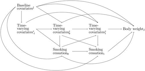
It is of paramount importance that the causal system is drawn based on background knowledge, and is not based on data availability. In this process, the omission of variables or arrows from the causal DAG is a stronger assumption than including them, as omissions of arrows amounts to constraining causal effects to exactly zero (Bollen & Pearl, 2013). In longitudinal studies, this might imply that not only lag-1 effects are included in the causal DAG, but also lag-2 and longer relations (VanderWeele, 2021). As encoded in the simplified causal DAG in Figure 1, we do not assume only lag-1 effects, but additionally allows for lag-2 effects and longer. This causal DAG does not assume any particular probability distribution for the causal system, nor does it specify the functional form of the causal relationships in the graph. This means that there may be linear but also non-linear relations, and that there may be interactions in addition to main effects.

We can now determine whether the causal estimand that was specified in Phase 1, can be expressed as a function of the observed data (i.e., the statistical estimand), given the background knowledge encoded in the causal DAG in Figure 1 and the available data. The causal identification assumption of consistency entails that the observed outcome of an individual who quits smoking for two years is equal to their potential outcome if quitting smoking for two years, that is, $Y_2^{{\overline{1}}_1}=Y$ for individuals with observed ${\overline{a}}_1={\overline{1}}_1.$ Similarly, the observed outcome of an individual who continues smoking for two years should be equal to their potential outcome if continuing smoking for two year, that is, $Y_2^{{\overline{0}}_1}=Y$ for individuals with observed ${\overline{a}}_1={\overline{0}}_1$ (Hernán & Robins, 2020). This seemingly obvious assumption implies that the exposure itself, as well as (hypothetical) interventions on it, must be sufficiently well defined such that it is clear what specific exposure the causal effect refers to (Hernán, 2016; VanderWeele, 2018). For example, smoking cessation can be achieved with the help of nicotine pills, therapy, a supporting friend, or a combination of these; setting the exposure to “quit smoking” leaves it open which of these exposures an individual undergoes. Because the different strategies might have different causal effects on body weight, the observed outcome need not necessarily equal the potential outcome. Information about the distribution of strategies to quit smoking might help to link the potential outcomes to observed data (Hernán & Robins, 2020), but this information is not collected in the LISS study, meaning that consistency is compromised in our example.

The conditional exchangeability assumption states that, given a set of covariates, the potential outcomes are independent of the observed exposures. In longitudinal settings, with multiple exposure-times, conditional exchangeability must hold at each time point. This can be denoted as $A_t\perp \text{}\perp Y^{{\overline{a}}_t}|{\overline{L}}_t,{\overline{A}}_{t-1}={\overline{a}}_{t-1},$ with ${\overline{L}}_t$ denoting the set of baseline and time-varying covariates up to and including time t and ${\overline{A}}_{t-1}={\overline{a}}_{t-1}$ representing the sequence of exposures a person received up to t − 1 (Hernán & Robins, 2020; Naimi et al., 2016). To be able to achieve this in practice, we must have collected data (without measurement error) on all relevant covariates that, based on the causal DAG, could confound the relationship between exposure and outcome. Based on Tian et al. (2015), ethnicity, socioeconomic factors, and energy intake were identified as relevant confounders. However, energy intake, for example, is not measured in the LISS data set, and therefore cannot be adjusted for in the analyses. As such, conditional exchangeability is compromised for our example. In practice, this conclusion would imply that additional data needs to be collected or identified to be able to provide a valid answer to the research question. Additionally, a sensitivity analysis can give insight into how strong the confounding by energy intake must be to substantively affect the conclusions derived from the primary analysis.

The sequential positivity assumption indicates that, at each time point and across all values of the covariates in the data, there is a non-zero probability for individuals to be in either exposure condition. This seems to be the case in this example on smoking cessation, because it is hard to conceive a policy or condition due to which an individual has a zero probability to quit or continue smoking.

Based on our evaluation of the causal identification assumptions for the empirical example, we conclude that additional data needs to be collected or identified to provide a valid answer to the causal research question: Such a finding is in itself is a useful contribution for the design of future studies (Petersen & Van der Laan, 2014). This example also underscores the importance of carefully considering Phases 1 and 2 in causal research before data is collected to ensure that the causal identification assumptions are as plausible as possible. If no additional data can be collected and the assumptions are compromised, then sensitivity analyses can be performed to determine, for example, how strong the relations of a confounding covariate must be to substantively change the conclusions of the primary analysis. For illustrative purposes we continue with the current example, but emphasize that causal interpretation of findings would be incorrect.

Using the causal identification assumptions, the causal estimand can be reexpressed as a statistical estimand. These steps, which are provided in detail in Appendix B, are a formalization of the causal identification process as described above. It yields: (4) $$\begin{array}{c}\text{causal estimand}:=\mathbb{E}[Y_2^{{\overline{1}}_1}]-\mathbb{E}[Y_2^{{\overline{0}}_1}],\\ ⋮\\ =\mathbb{E}\{\mathbb{E}(\mathbb{E}[Y_2|{\overline{A}}_1={\overline{1}}_1,{\overline{L}}_1]|A_0=1,L_0)\}\\ \mathrm{\hspace{1em}}\mathrm{\hspace{1em}}-\mathbb{E}\{\mathbb{E}(\mathbb{E}[Y_2|{\overline{A}}_1={\overline{0}}_1,{\overline{L}}_1]|A_0=0,L_0)\}\\ =:\text{statistical estimand}.\end{array}$$(4) Notice how the identification process starts with the causal estimand in terms of potential outcomes (hypothetical quantities), and ends in a statistical estimand with only observed variables. However the statistical estimand in Equation (4)(4) $$\begin{array}{c}\text{causal estimand}:=\mathbb{E}[Y_2^{{\overline{1}}_1}]-\mathbb{E}[Y_2^{{\overline{0}}_1}],\\ ⋮\\ =\mathbb{E}\{\mathbb{E}(\mathbb{E}[Y_2|{\overline{A}}_1={\overline{1}}_1,{\overline{L}}_1]|A_0=1,L_0)\}\\ \mathrm{\hspace{1em}}\mathrm{\hspace{1em}}-\mathbb{E}\{\mathbb{E}(\mathbb{E}[Y_2|{\overline{A}}_1={\overline{0}}_1,{\overline{L}}_1]|A_0=0,L_0)\}\\ =:\text{statistical estimand}.\end{array}$$(4) is just one “form,” known in the causal inference literature as the “g-formula representation,” but can be further rewritten such that it takes a different form (for an introduction to the parametric g-formula aimed at psychological researchers, see Loh et al., 2023). This is illustrated in Appendix B where we further rewrite the g-formula representation of the statistical estimand to the “IPW representation.” Different representations of a statistical estimand invite different modeling approaches for Phase 3, and this can have advantages (or disadvantages) for particular research designs.

3.3. Phase 3: Estimation Using Finite Sample Data

The terms in the statistical estimand can be estimated from finite random samples (taken from the population distribution) under a statistical model. The “g-formula representation” of the statistical estimand in Equation (4)(4) $$\begin{array}{c}\text{causal estimand}:=\mathbb{E}[Y_2^{{\overline{1}}_1}]-\mathbb{E}[Y_2^{{\overline{0}}_1}],\\ ⋮\\ =\mathbb{E}\{\mathbb{E}(\mathbb{E}[Y_2|{\overline{A}}_1={\overline{1}}_1,{\overline{L}}_1]|A_0=1,L_0)\}\\ \mathrm{\hspace{1em}}\mathrm{\hspace{1em}}-\mathbb{E}\{\mathbb{E}(\mathbb{E}[Y_2|{\overline{A}}_1={\overline{0}}_1,{\overline{L}}_1]|A_0=0,L_0)\}\\ =:\text{statistical estimand}.\end{array}$$(4) suggests that we impose a statistical model on the distribution of the outcome given the exposure and covariate history, and thus assumes that we accurately model the relationships between the outcome and the covariates (Schafer & Kang, 2008). In contrast, the statistical estimand can be reexpressed (see Appendix B) to the IPW representation, such that it does not suggest that the conditional distribution of the outcome be modeled; instead, the reexpressed statistical estimand suggests that the time-varying exposures are modeled. So the same causal effect can be expressed as two different representations of a statistical estimand, each of which invites a different modeling strategy, and depending on a particular application one modeling strategy might be advantageous over the other. Here, we compare path analysis to IPW estimation—in which path analysis is more in line with the g-formula representation of the statistical estimand, and IPW estimation (obviously) with the IPW representation (Naimi et al., 2016)—and attempt to answer our research question using the LISS data.

3.3.1. Establishing the Study Sample from the LISS Data

The LISS panel study is based on a rolling enrollment, meaning that each year, a new group of individuals is added to the existing participant pool. Table 2 contains an overview of covariates that were included in the LISS data. We established the study sample for the target population “currently smoking Dutch adults” from the LISS data as follows. From each participant, the first four yearly measures were selected (regardless of the year in which participants enrolled), corresponding to time anchors t = − 1 to t = 2 in our study. If participants indicated affirmatively on the question “Do you smoke now?” at their first measurement wave, they were included in the sample of this study starting from the wave after (i.e., their second measurement wave is at t = 0). The sample included 2,736 participants. Participants with implausible or impossible values on variables were deleted (i.e., weight higher than 200 kg or lower than 20 kg, yearly weight increase followed by weight decrease of more than 50 kg, more than 150 h of physical activity per week). To keep the focus of this analysis on the parametric assumptions underlying both approaches, we filled in missing values in this sample by single imputation using the mice package (version 3.16.0; Buuren & Groothuis-Oudshoorn, 2011) in R (version 4.2.2; R Core Team, 2022).

Table 2. Overview of covariates included in the LISS panel study.

Covariate	Measurement level	Measurement time	Time-span
Age	Continuous	Baseline	Right now
Sex	Nominal	Baseline	Right now
Body weight	Continuous	Time-varying	Right now
Alcohol consumption	Ordinal	Time-varying	Average last year
Hours physical activity	Continuous	Time-varying	Average last week
Number of comorbidities^a	Ordinal	Time-varying	Last year

Note. All variables are self-reported measures taken from a questionnaire.

^a Self reported information on diagnosis by a physician.

3.3.2. Path Analysis with an Additional Joint Effect Parameter

In a typical SEM approach, the entire causal system as illustrated in the simplified DAG of Figure 1 would be interpreted as a path diagram. This implies that each dependency is specified in a SEM model as a linear effect, with independent residuals that are multivariate normally distributed. All exogenous variables (i.e., the baseline covariates) are allowed to freely covary with each other. This path diagram represents a set of linear equations, the parameters of which are estimated from the data. If the entire causal system is correctly specified (i.e., all dependencies in Figure 1 are indeed linear; there is no measurement error, effect modification, or interactions between the intermediate covariates in influencing the outcome; error terms follow a multivariate normal distribution; Gische & Voelkle, 2022), then this approach results in unbiased estimates of each path. Estimates of our joint effect of interest can then be obtained as linear combinations of path-specific estimates. In particular, the joint effect is a linear combination of all regression coefficients on paths from exposures (both at time points 0 and 1) to the outcome, not going through later exposures. For the empirical example, this includes (a) the lag-2 path “Smoking cessation₀” → “Body weight₂”; (b) the set of indirect paths “Smoking cessation₀” → “Time-varying covariates₁” → “Body weight₂”; and (c) the path “Smoking cessation₁” → “Body weight₂.” The combinations of these paths can be specified as additional parameters in a SEM model, such that point estimates for the targeted effects can be obtained directly. Confidence intervals can be obtained by nonparametric bootstrap.

A complicating factor is the inclusion of time-varying covariates that are categorical. When the effect of exposure on an intermediate time-varying covariate is estimated based on logistic or probit regression, it results in a logit or probit coefficient, and the simple product of regression coefficients along causal paths should not be used (Li et al., 2007). Some solutions have been proposed in the causal mediation literature, such as the use of adjusted logit and probit regression estimates when taking the product of regression coefficients (Li et al., 2007), or estimation of so-called counterfactually-defined indirect effects based on the simulation of potential outcomes (B. O. Muthén et al., 2016; Nguyen et al., 2016). However, the uptake up these methods is limited (Rijnhart et al., 2023), and these methods have not been implemented and evaluated for cross-lagged panel research yet. For this reason, a path analysis using the LISS data that incorporates all variables mentioned in Table 2, including those covariates measured in a categorical manner (e.g., alcohol consumption, number of comorbidities), is currently not a viable option.

For purely illustrative purposes, we discard the categorical covariates in this example such that we can continue our comparison of SEM and potential outcome approaches, and (the impact of) the parametric assumptions underlying path analysis and IPW estimation. We stress that this decision is far from satisfying from a causal inference point-of-view because the exchangeability assumption would consequently be violated. The decision is a necessary consequence of choosing path analysis as an estimation strategy in this phase. A path model based on Figure 1 was fitted to the LISS data in Mplus version 8.9. (L. K. Muthén & Muthén, 2017). Only body weight and hours of physical activity were included as time-varying covariates. The probit-link was used for regressing the time-varying exposures on covariates.

3.3.3. IPW Linear Regression

In brief, the aim of IPW is to create a pseudo-population in which the exchangeability assumption holds conditional on the measured covariates (Robins et al., 2000). This is achieved in three steps. First, probability of exposure is estimated using a propensity score model in which the exposure is regressed on the measured confounding variables. For a categorical exposure, such a model is commonly a logistic regression model in which the exposure is the outcome, and all confounding variables identified using the approach described in Section 3.2 are independent variables. The propensity score model must be correctly specified, implying that the functional form of the dependencies in the model is correct (i.e., the dependencies are in fact linear). In the second step, inverse-probability-of-exposure-weights are created for each individual. These are based on the probability of observed exposures values from the fitted propensity score model, which are inverted, and then multiplied across the time points per individual. The resulting weights are used to balance the original sample: Individuals with a low probability of scoring their observed exposure value have a higher weight, and are therefore over-represented in the pseudo-population, whereas individuals with a high probability of scoring their observed exposure have a lower weight, and are therefore underrepresented in the pseudo-population. The consequence of this weighting procedure is that in the pseudo-population the dependencies of the time-varying exposure on the time-varying varying-covariates—the paths “Time-varying covariates${}_{-1}$” → “Smoking cessation₀”; “Time-varying covariates${}_{-1}$” → “Smoking cessation₁”; “Time-varying covariates₀” → “Smoking cessation₀”; “Time-varying covariates₀” → “Smoking cessation₁”; and “Time-varying covariates₁” → “Smoking cessation₁”—are broken, such that these covariates are not confounders anymore for the effect of smoking cessation on end-of-study body weight. In the third step, estimates of the targeted effects are obtained by fitting a weighted regression model to the pseudo-population in which the outcome is regressed on both exposure-times. If the parametric assumptions (e.g., linearity, the absence of interaction effects) of this outcome model hold, then this procedure leads to unbiased estimates of the effect of exposure at time point 0 not going through later exposures, and exposure at time point 1, on the outcome. These effects of smoking cessation at each time point are also sometimes referred to as controlled direct effects, where the term “controlled” refers to controlling for future exposures, and “direct” refers to the fact that the intermediate process by which smoking cessation leads to body weight is not modeled (Daniel et al., 2013). The sum of both controlled direct effects is our estimate of the joint effect.

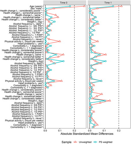
The IPW regression method was applied to our empirical example. In contrast to path analysis, we include both categorical and continuous time-varying covariates here. A propensity score model was fitted by regressing the exposure variables on covariate history and previous exposure status. Positivity was evaluated by a visual inspection of overlap of the distributions of propensity scores of exposed and non-exposed at each time point, see Figure 2. No violation to positivity was detected. Stabilized IPWs were computed from the propensity score model using the R package WeightIt (version 0.14.0; Greifer, 2023b). Balance of the confounding variables in the propensity score model was assessed by comparing the standardized means of covariates for those who quit smoking, and those who continued smoking, using the R package cobalt (version 4.5.0; Greifer, 2023a). This comparison was done in both the unweighted sample and the weighted sample (i.e., the pseudo-population), and at both exposure-times, see Figure 3. Absolute standardized mean differences indicated well-balanced data based on a recommended threshold value of 0.2 (Stuart, 2010).

Figure 2. Density of propensity scores for individuals who quit smoking versus individuals who continued smoking at time points 0 and 1 (before weighting). Propensity scores were computed using all covariates.

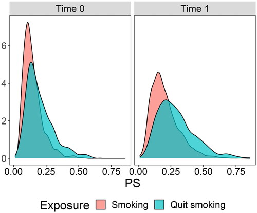
Figure 3. Visualization of covariate balance (standardized mean differences) before and after reweighing at time points 0 and 1. The asterisk * denotes binary covariates (or dummy variables) for which the displayed value is the raw (unstandardized) difference in means. PW = per week; PM = per month; P2M = per two months; PY = per year.

A regression model was fitted to the pseudo-population, regressing body weight at t = 2 on smoking cessation at t = 0 and t = 1. The regression coefficients of smoking cessation at t = 0 and $t=1$ are the controlled direct effects, the combination of which is our joint effect of interest. 95% confidence intervals were obtained using the nonparametric bootstrap with 999 replications. Bootstrapping was performed using the R package boot (version 1.3-28; Canty & Ripley, 2022).

3.3.4. Results

Path analysis resulted in an estimated always-exposed versus never-exposed effect of 0.69, 95% CI [−0.01, 1.34], implying that there is no evidence of an effect of sustained smoking cessation on body weight a year later. Analysis with IPW regression resulted in a negative estimate of sustained smoking cessation, −1.87, [−4.29, 0.53], although it similarly was not significant at the $\alpha =.05$ level. Although the conclusions drawn in terms of significance would be the same for this particular empirical example, both methods resulted in wildly different point estimates (the point estimate of one method is not contained within the confidence interval of the other). This difference can be due to the different set of covariates that was adjusted for, and the different parametric assumptions that both methods rely on. Note again that the results from IPW regression are based on a limited set of covariates that is adjusted for due to unavailability in the LISS data, and that results from the path analyses are based on a smaller set of covariates due to the limitations of including a large set of (categorical) covariates into a SEM model. When more covariates are included in the analyses, the results in terms of point estimates and significance can change, and it is not possible to predict beforehand how (dis)similar results from both methods will be for any given application.

4. Simulation Study

So far, we have given an elaborate illustration of the investigation of joint effects, specifically an always-exposed versus never-exposed effect, in the causal inference framework, and using path analysis and IPW linear regression as estimation methods. In the current section, we study the impact of violations of parametric assumptions in path analysis and IPW linear regression, particularly, violations of the linearity assumption. We performed a simulation study to compare the finite sample performance of both estimation methods in terms of bias and MSE under various scenarios of model misspecification. In line with the empirical example, we focused on investigating the always-exposed versus never-exposed effect. The scenarios considered here were further simplified compared to the empirical example (in terms of number of covariates), but are based on the same causal structure as the simplified DAG in Figure 1.

4.1. Data Generation

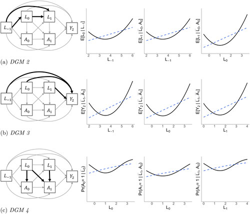
Data were generated under five different data-generating mechanisms (DGMs). All DGMs contain a time-varying binary exposure A measured at time points t = 0, 1, a continuous end-of-study outcome Y₂, a continuous baseline confounder $L_{-1},$ and continuous time-dependent confounding variables L_t at time points $t=0,1.$ The simulated data have a causal structure as visualized in Figure 4, with continuous variables following a normal distribution. Appendix A contains a table with population values for all regression coefficients. In DGM 1, all dependencies are linear. In DGM 2, the dependencies of the time-dependent confounders L₀ and L₁ include a quadratic term, see Figure 5(a). These terms were created by first grand mean centering the predictors before squaring them. The quadratic regression coefficients were equal to the linear regression coefficients. By grand mean centering the predictors, the population value of the always-exposed versus never-exposed effect does not change. In DGM 3, the dependencies of the outcome on the baseline and time-dependent covariates are quadratic, see Figure 5(b). In DGM 4, the dependencies of the exposure on the time-varying covariates are quadratic, see Figure 5(c). Finally, DGM 5 combines all quadratic dependencies of DGMs 2, 3 and 4. In all five DGMs, the population controlled direct effect of A₀ on Y₂ is 0.32, and the population controlled direct effect of A₁ on Y₂ is 0.40, such that, combined, the population always-exposed versus never-exposed effect is 0.72. Data generation was performed in base R (version 4.2.2; R Core Team, 2022).

Figure 4. The causal structure of the data generating mechanisms used in the simulations.

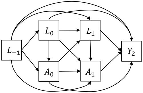
Figure 5. Overview of data generating mechanisms (DGMs) 2, 3, and 4. Bold black arrows in the DAGs indicate nonlinear dependencies. These direct effects are visualized in the plots to the right of each respective DGM, with the solid black line representing the true (nonlinear) functional relationship between two variables, and the dashed blue line representing the linear projection. DGM 1 (not illustrated here) contains only linear dependencies. DGM 5 (not illustrated here) combines the nonlinear dependencies of DGMs 2, 3, and 4.

4.2. Estimation

Five different estimation methods were used for investigating the always-exposed versus never-exposed effect: IPW linear regression, linear path analysis, IPW regression with both linear and quadratic terms in the propensity score model, path analysis with both linear and quadratic terms, and linear regression without confounding adjustment. These methods estimated the always-exposed versus sustained non-exposed effect as a combination of the controlled direct effects of A₀ and A₁. The propensity score model and outcome model of IPW linear regression were fitted using standard OLS regression in R version 4.2.2 (R Core Team, 2022). The path analysis models were fitted in Mplus version 8.9, with the probit link used for the regression models of the exposures, and robust maximum likelihood selected as the estimator (L. K. Muthén & Muthén, 2017).

The linear IPW estimation method was misspecified under DGMs 4 and 5: It wrongly assumed linear dependencies for the propensity score model. For path analysis, a linear path analysis model was specified, which was locally misspecified under DGMs 2, 3, 4, and 5. To get a sense for the impact of misspecification on performance of the method, we also estimated the joint effects without misspecification in the methods: For IPW, this was implemented using a propensity score model that included quadratic terms for DGMs 4 and 5; for path analysis, a path analysis model was specified which included quadratic terms where relevant for DGMs 2, 3, 4, and 5. These latter two scenarios thus represent a “best-case scenario,” in which no model misspecification occurs in the IPW regression, and path analysis methods. Finally, a linear regression model with Y₂ as the outcome and A₀ and A₁ as independent variables was specified, without any regression adjustment for confounding, or weighting. This method provides a benchmark for a “worst-case scenario” against which we can compare (misspecified) IPW regression and path analysis methods. Performance of these five methods under different simulation conditions was evaluated in terms of bias of the joint-effect point estimates, and mean square error (MSE).

In addition to varying the source of model misspecification, we varied sample size (n = 300, 1,000) and proportion exposed at both time points ($p=0.1,0.5,0.9$). Combined, this lead to 30 simulation conditions. For each condition, a thousand replications were simulated.

5. Results

Figure 6 visualizes the bias of point estimates for the always-exposed versus never-exposed effect across the five estimation methods. Here, we only present results for a sample size of n = 1,000, and 10% and 50% exposed. Figure 7 contains the mean square error of these point estimates. The horizontal bars in both plots are 95% confidence intervals (CI), based on Monte Carlo standard errors, for the bias and MSE (Morris et al., 2019). For most estimates of bias and MSE, this CI is so narrow that it is not visible. Numerical results, as well as results for the other simulation conditions, are included in the online supplementary materials.

Figure 6. Bias in the point estimates of the always-exposed versus never-exposed effect across five methods: “IPW (L)” is linear IPW regression; “path (L) is linear path analysis; “IPW (L, Q)” is IPW regression with linear and quadratic terms in DGMs 3, 4, and 5; “path (L, Q)” is path analysis with linear and quadratic terms in DGMs 2, 3, 4, and 5; “unadjusted” is a linear regression without confounding adjustment. Results are presented for the case of n = 1,000, 10% and 50% exposed, and across five DGMs.

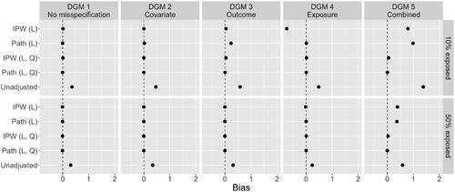
Figure 7. MSE of the point estimates of the always-exposed versus never-exposed effect across five methods, and five DGMS (n = 1,000).

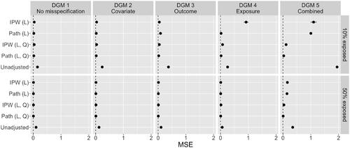
As expected under DGM 1, the linear IPW regression model and linear path analysis model performed well in terms of bias and MSE. Here, the IPW regression model and path analysis model with additional quadratic effects were equivalent, as all dependencies are in fact linear under DGM 1. For DGM 2, there was only slight upward bias for the linear path analysis model under the 10% exposed condition, which reduced to near 0 when exposure was balanced (it is barely visible in Figure 6, but shows in the numerical results in the online supplementary materials). This bias did not exist for the linear IPW regression model, although it had more variability of the estimates as reflected in the slightly increased MSE.

Results for DGM 3 and 10% exposed showed significant bias in the estimates of the linear path analysis model, and small bias for the linear IPW regression model. The higher bias for the linear path analysis model was also reflected in the MSE, which was now higher than that of the linear IPW regression model. When exposure was balanced, these biases disappeared and linear path analysis had a lower MSE again. Results for DGM 4 with 10% exposed showed a large negative impact of an incorrectly specified propensity score model for IPW-based estimators (Hernán & Robins, 2020). There was considerable bias for the linear IPW regression model and increased MSE. When exposure was balanced in the sample, both bias and MSE were close to zero again, although some bias remained. Somewhat surprisingly, estimates of the effect of interest in the linear path analysis model appeared unaffected by the incorrectly modeled exposures, with no bias and low MSE for both the 10% exposed and 50% exposed conditions.

Finally, for DGM 5, both the linear IPW regression model and the linear path analysis model performed badly, with significant bias in the point estimates and high MSE. This was expected as there was considerable misspecification of functional forms in multiple locations of the models (i.e., numerous violations of parametric assumptions). Performance increased somewhat when the proportion exposed in the sample was balanced, but bias remained significant. In this situation, both methods performed almost as poorly as the naive, unadjusted method.

6. Discussion

While the use of SEM models for causal inference from longitudinal observational data is quite popular in psychology, this practice has been criticized in the causal inference literature for its high potential of model misspecification and, consequently, bias in the estimates of causal effects of interest (cf. Bollen & Pearl, 2013; Van der Laan & Rose, 2011; VanderWeele, 2012). To fully understand this critique, and to see why the alternative causal inference methods that have been proposed counter these problems, researchers need to be knowledgeable of the potential outcomes framework. Although SEM methods are compatible with the potential outcomes framework (e.g., Loeys et al., 2014; Moerkerke et al., 2015; B. O. Muthén et al., 2016), the literature on the potential outcomes framework comes predominantly from the disciplines of epidemiology and biostatistics; as such, the literature is targeted to research problems and common practices that psychological researchers are less familiar with, making it difficult to bridge the disciplinary gap. In this article, we first introduced SEM users from psychology (and related disciplines) to three core phases of the potential outcomes approach to causal inference (inspired by Goetghebeur et al., 2020; Petersen & Van der Laan, 2014). In particular, we compared path analysis from the SEM framework to IPW estimation of MSMs in the context of cross-lagged panel research, and when investigating an always-exposed versus never-exposed effect of a time-varying exposure on an end-of-study outcome in the presence of baseline and time-varying confounding. Through the use of a simulation study, we assessed the finite-sample performance (in terms of bias and MSE) of both methods under varying violations of parametric assumptions.

Simulation results showed that, for the specific scenarios investigated in this study, path analysis generally had lower MSE than IPW estimation when estimating the time-varying exposure effect; the only exception here was for DGM 3, with misspecification in the relationships between the confounders and the outcome. The lower MSE obtained with path analysis was mainly due to higher efficiency obtained from making assumptions about the relationships between variables, which compensated for the higher bias under particular forms of misspecification (see, for example, the lower MSE of path analysis in DGM 4, specifically for “IPW (L, Q)” and “Path (L, Q)”; and DGM 5, even while path analysis was as biased, or more biased than IPW regression). For misspecification of the covariate-outcome relations (i.e., in DGM 3, in which a linear relation was assumed in the fitted model whereas data were generated under a quadratic relation), results for an uneven distribution of exposed and non-exposed individuals (10% exposed) confirmed that path analysis was more prone to bias in the always-exposed versus never-exposed effect than IPW estimation. However, the bias appeared to be minor. For misspecification of the propensity score model (the covariate-exposure relationships in DGM 4), IPW estimation led to significant bias for the always-exposed versus never-exposed effects, whereas no bias was observed for path analysis in this scenario. When covariate, exposure, and outcome dependencies were all misspecified (DGM 5), then both path analysis and IPW regression performed almost as poorly (in terms of bias) as standard linear regression without any covariate adjustment. Interestingly, bias across all scenarios was significantly reduced when the proportion exposed was balanced.

Hence, our comparison of path analysis and IPW estimation across the three phases of causal inference has made insightful how SEM approaches fit within a principled approach to causal inference, the causal identification assumptions that both methods rely on, and the differences between them in terms of the parametric assumptions they make. Subsequently, our simulations have shown that violations of parametric assumptions unique to path analysis (i.e., concerning covariate-covariate relationships, investigated in DGM 2; and covariate-outcome relationships, investigated in DGM 3) do not always translate into substantial bias when estimating joint effects from finite samples. These results nuance the criticism of SEM for the purpose of causal inference, for instance as expressed by VanderWeele (2012). Moreover, we find that in a setting without unmeasured confounding, path analysis actually performed better generally in terms of MSE, and showed no bias when the functional forms of the covariate-exposure relations are misspecified, in contrast to IPW estimation (see DGM 4).

However, this should not be interpreted to mean that SEM can be easily used in cross-lagged panel research for the purpose of causal inference. First, our illustrative example highlights that attempts to model the entire data generating mechanism (as with cross-lagged panel modeling approaches) complicates computations of joint effects when categorical time-varying covariates are included (e.g., combining linear regression coefficients with logit or probit coefficients). This is problematic as the inclusion of many time-varying covariates is required to make the causal identification assumption of conditional exchangeability plausible in the first place, and some covariates are likely to be categorical in practice (e.g., level of education, diagnoses of psychological disorders, relationship status, etc.). Second, our simulations focused only on a limited number of scenarios in which the violation of parametric assumptions was limited to the omission of a quadratic term. We are likely to find more extreme biases for both methods under more severe violations in which linear relationships cannot approximate the true functional relationship well (for example, see Table 1 of Kang & Schafer, 2007). In such situations, the use of machine learning techniques for fitting nonparametric models is advisable, and IPW-based methods have been extended to easily allow for this (Greifer, 2023b). Third, the presence of unmeasured confounding variables, wrongfully omitting interactions and second-order lagged effects from the model, and a different set of population parameter values are factors that have not been explored in these simulations, but which can have a profound impact on the performance of both methods. In light of this uncertainty, it is therefore generally advisable to consider methods that relax the parametric assumptions as much as possible, and causal inference methods from the potential outcomes framework are advantageous in this respect compared to various kinds of cross-lagged panel models.

Furthermore, we emphasize that these simulation results should certainly not be interpreted as an incentive to continue currently popular SEM modeling practices, when the actual goal is causal inference. While estimation of causal effects using SEM models can work well for carefully-defined research problems (as illustrated by the relatively good performance of path analysis across different scenarios in the simulations, especially in terms in MSE), it requires careful and elaborate consideration of the issues and topics in Phases 1 and 2 of causal research, as we have shown in this article. Fitting an off-the-shelf bivariate cross-lagged panel model (or a related SEM-model) without inclusion of additional covariates (both baseline and time-invariant), and without consideration of lag-2 and further relationships, is inappropriate for investigating causal effects. While this paper focused on the investigation of joint effects, our conclusion equally applies when the interest is in cross-lagged effects. In fact, we estimated joint effects as combinations of CDEs, and under the causal DAGs in Figures 1 and 4, the CDE of exposure at time point 2 is the same as the cross-lagged effect of exposure at time point 2 to the end-of-study outcome. Psychological researchers are therefore well-advised to study the potential outcomes framework, and the proposed causal inference methods therein such that they can make better-informed decisions about which modeling approach is appropriate given their considerations in Phases 1 and 2.

In this article, we limited our simulations to misspecification of functional forms, and did not investigate the impact of unobserved confounding variables from the analysis, or the potential of latent variables to (partially) adjust for this (Usami et al., 2019). Unobserved confounding is, however, a fundamental issue in causal research. We also did not study the performance of path analysis and IPW estimation under violations of conditional independence assumptions—that is, when the causal DAG that acts as the basis for our analyses wrongfully omits one, or multiple, dependencies—which was an additional critique in VanderWeele (2012). Instead, in our simulations and in our illustrative example, both the path analysis model and IPW estimation included lag-0, lag-1, lag-2, and lag-3 relationships. Furthermore, missingness in the illustrative example was handled by single stochastic imputation for practical reasons. However, as the SEM framework and potential outcome framework have different techniques for missing data handling—IPW for censoring is more common in the potential outcomes framework, whereas the use of full information likelihood is widespread in SEM—it would be interesting to also investigate how differences in these techniques impact estimation performance.

In conclusion, psychological research has fully embraced the SEM framework for causal inference, whereas the uptake of the potential outcomes framework, and the causal inference methods developed herein, has been lagging behind. However, reduced reliance on parametric assumptions and the possibility to include a large set of (categorical) time-varying covariates, are good reasons to invest time in learning techniques such as IPW estimation of MSMs. We hope this comparison of IPW estimation and path analysis facilitates a better understanding of these methods for causal inference about time-varying exposure effects.

Additional information

Funding

Mulder and Hamaker are part of the Consortium on Individual Development (CID). CID is funded through the Gravitation Program of the Dutch Ministry of Education, Culture, and Science and the Netherlands Organization for Scientific Research (NWO grant number 024.001.003).

Notes

1 Readers more familiar with the potential outcomes literature might recognise this research question as pertaining to static exposure regimes rather than dynamic exposure regimes. For accessibility of the paper, we focus exclusively on the simpler case of static exposure regimes.

2 We discuss parametric assumptions in Phase 3, but it is possible that parametric assumptions are already incorporated in the statistical estimand, and are thus part of Phase 2. A more estimation-specific (i.e., Phase 3-specific) matter is how the parameters of the statistical models are estimated using finite samples. Different estimators (e.g., maximum likelihood with or without penalization, or random forests) need not have the same statistical properties (e.g., finite sample bias, statistical convergence, sampling variability).

Appendix A

A1. Simulation Study

Table A1 contains the population values used for data generation. $L_{-1}$ is normally distributed with mean 4 and variance 1. Residuals are standard-normally distributed. The intercepts of L₀ and L₁ are set to 1. The intercept of Y₂ is 0. These population values resulted in an always-exposed versus never-exposed effect of 0.72.

Table A1. Population values used for data generation.

Causal effect	Population value
$L_{-1}\to \dots$	0.1^a
$L_0\to A_0$	0.5
$L_0\to L_1$	0.3
$L_0\to A_1$	0.25
$L_0\to Y_2$	0.15
$A_0\to L_1$	0.4
$A_0\to A_1$	0.8
$A_0\to Y_2$	0.2
$L_1\to A_1$	0.5
$L_1\to Y_2$	0.3
$A_1\to Y_2$	0.4

^a This value applies to all effects of $L_{-1}.$

Appendix B

B1. Derivation Statistical Estimand

Here, we describe the derivation of the statistical estimand in Equation (4)(4) $$\begin{array}{c}\text{causal estimand}:=\mathbb{E}[Y_2^{{\overline{1}}_1}]-\mathbb{E}[Y_2^{{\overline{0}}_1}],\\ ⋮\\ =\mathbb{E}\{\mathbb{E}(\mathbb{E}[Y_2|{\overline{A}}_1={\overline{1}}_1,{\overline{L}}_1]|A_0=1,L_0)\}\\ \mathrm{\hspace{1em}}\mathrm{\hspace{1em}}-\mathbb{E}\{\mathbb{E}(\mathbb{E}[Y_2|{\overline{A}}_1={\overline{0}}_1,{\overline{L}}_1]|A_0=0,L_0)\}\\ =:\text{statistical estimand}.\end{array}$$(4) from the causal estimand in Equation (1)(1) $$\text{ACE}=\mathbb{E}\left[Y_2^{{\overline{1}}_1}\right]-\mathbb{E}\left[Y_2^{{\overline{0}}_1}\right].$$(1) . In the derivation we repeatedly make use of laws of conditional expectations (see Chapter 10 of Steyer & Nagel, 2017), as well as the causal identification assumptions of conditional exchangeability, consistency, and positivity. Equality (1) follows from the law of iterated expectations with regards to L₀. Equality (2) follows from the conditional exchangeability assumption of the form $Y_2^{{\overline{a}}_1}\perp \text{}\perp A_0|L_0,$ and from the positivity assumption with regards to A₀, $\mathit{\text{Pr}}[a_0|l_0]>0,$ for all l₀. Equality (3) follows from law of iterated expectations with regards to L₁, conditional on L₀ and A₀. As we now condition on both L₀ and L₁, we represent this as conditioning on covariate history ${\overline{L}}_1.$ Equality (4) follows from conditional exchangeability of the form $Y_2^{{\overline{a}}_1}\perp \text{}\perp A_1|{\overline{L}}_1,A_0=a_0,$ and the positivity assumption with regards to A₁, $\mathit{\text{Pr}}[a_1|a_0,{\overline{l}}_1]>0,$ for all a₀ and ${\overline{l}}_1.$ Equality (5) relies on the consistency assumption, stating that $Y_2^{{\overline{1}}_1}=Y_2$ for individuals with observed ${\overline{A}}_1={\overline{1}}_1,$ and $Y_2^{{\overline{0}}_1}=Y_2$ for individuals with observed ${\overline{A}}_1={\overline{0}}_1.$ $$\text{causal estimand}:=\mathbb{E}[Y_2^{{\overline{1}}_1}]-\mathbb{E}[Y_2^{{\overline{0}}_1}],{\displaystyle \stackrel{(1)}{=}}\mathbb{E}\{\mathbb{E}[Y_2^{{\overline{1}}_1}|L_0]\}-\mathbb{E}\{\mathbb{E}[Y_2^{{\overline{0}}_1}|L_0]\}{\displaystyle \stackrel{(2)}{=}}\mathbb{E}\{\mathbb{E}[Y_2^{{\overline{1}}_1}|A_0=1,L_0]\}-\mathbb{E}\{\mathbb{E}[Y_2^{{\overline{0}}_1}|A_0=0,L_0]\}\stackrel{(3)}{=}\mathbb{E}\{\mathbb{E}(\mathbb{E}[Y_2^{{\overline{1}}_1}|A_0=1,{\overline{L}}_1]|A_0=1,L_0)\}\mathrm{\hspace{1em}}\mathrm{\hspace{1em}}-\mathbb{E}\{\mathbb{E}(\mathbb{E}[Y_2^{{\overline{0}}_1}|A_0=0,{\overline{L}}_1]|A_0=0,L_0)\}\stackrel{(4)}{=}\mathbb{E}\{\mathbb{E}(\mathbb{E}[Y_2^{{\overline{1}}_1}|{\overline{A}}_1={\overline{1}}_1,{\overline{L}}_1]|A_0=1,L_0)\}\mathrm{\hspace{1em}}\mathrm{\hspace{1em}}-\mathbb{E}\{\mathbb{E}(\mathbb{E}[Y_2^{{\overline{0}}_1}|{\overline{A}}_1={\overline{0}}_1,{\overline{L}}_1]|A_0=0,L_0)\}\stackrel{(5)}{=}\mathbb{E}\{\mathbb{E}(\mathbb{E}[Y_2|{\overline{A}}_1={\overline{1}}_1,{\overline{L}}_1]|A_0=1,L_0)\}\mathrm{\hspace{1em}}\mathrm{\hspace{1em}}-\mathbb{E}\{\mathbb{E}(\mathbb{E}[Y_2|{\overline{A}}_1={\overline{0}}_1,{\overline{L}}_1]|A_0=0,L_0)\}=:\text{statistical estimand} (\text{g‐formula representation}).$$

This statistical estimand takes the form that is known in the causal inference literature as the standard g-formula for time-varying exposures (Loh et al., 2023; Naimi et al., 2016; Robins, 1986). It can be further rewritten to a form that is known in the causal inference literature as the IPW representation. Continuing from the statistical estimand in g-formula representation on the right-hand side of Equality (5), it yields: $$\mathbb{E}\{\mathbb{E}(\mathbb{E}\left[Y_2\right|{\overline{A}}_1={\overline{1}}_1,{\overline{L}}_1\left]\right|A_0=1,L_0)\}\mathrm{\hspace{1em}}\mathrm{\hspace{1em}}-\mathbb{E}\{\mathbb{E}(\mathbb{E}\left[Y_2\right|{\overline{A}}_1={\overline{0}}_1,{\overline{L}}_1\left]\right|A_0=0,L_0)\}\stackrel{(6)}{=}\mathbb{E}\{\mathbb{E}(\mathbb{E}\left[\frac{Y_2\mathbb{1}(A_1=1)}{\mathrm{\text{Pr}}(A_1=1|A_0=1,{\overline{L}}_1)}\right|A_0=1,{\overline{L}}_1\left]\right|A_0=1,L_0)\}\mathrm{\hspace{1em}}\mathrm{\hspace{1em}}-\mathbb{E}\{\mathbb{E}(\mathbb{E}\left[\frac{Y_2\mathbb{1}(A_1=0)}{\mathrm{\text{Pr}}(A_1=0|A_0=0,{\overline{L}}_1)}\right|A_0=0,{\overline{L}}_1\left]\right|A_0=0,L_0)\}\stackrel{(7)}{=}\mathbb{E}\{\mathbb{E}(\frac{Y_2\mathbb{1}(A_1=1)}{\mathrm{\text{Pr}}(A_1=1|A_0=1,{\overline{L}}_1)}|A_0=1,L_0)\}\mathrm{\hspace{1em}}\mathrm{\hspace{1em}}-\mathbb{E}\{\mathbb{E}(\frac{Y_2\mathbb{1}(A_1=0)}{\mathrm{\text{Pr}}(A_1=0|A_0=0,{\overline{L}}_1)}|A_0=0,L_0)\}\stackrel{(8)}{=}\mathbb{E}\{\mathbb{E}(\frac{Y_2\mathbb{1}({\overline{A}}_1={\overline{1}}_1)}{\mathrm{\text{Pr}}(A_0=1|L_0)\mathrm{\text{Pr}}(A_1=1|A_0=1,{\overline{L}}_1)}|L_0)\}\mathrm{\hspace{1em}}\mathrm{\hspace{1em}}-\mathbb{E}\{\mathbb{E}(\frac{Y_2\mathbb{1}({\overline{A}}_1={\overline{0}}_1)}{\mathrm{\text{Pr}}(A_0=0|L_0)\mathrm{\text{Pr}}(A_1=0|A_0=0,{\overline{L}}_1)}|L_0)\}\stackrel{(9)}{=}\mathbb{E}\left\{\frac{Y_2\mathbb{1}({\overline{A}}_1={\overline{1}}_1)}{\mathrm{\text{Pr}}(A_0=1|L_0)\mathrm{\text{Pr}}(A_1=1|A_0=1,{\overline{L}}_1)}\right\}\mathrm{\hspace{1em}}\mathrm{\hspace{1em}}-\mathbb{E}\left\{\frac{Y_2\mathbb{1}({\overline{A}}_1={\overline{0}}_1)}{\mathrm{\text{Pr}}(A_0=0|L_0)\mathrm{\text{Pr}}(A_1=0|A_0=0,{\overline{L}}_1)}\right\}\stackrel{(10)}{=}\mathbb{E}[W{Y}_2\mathbb{1}({\overline{A}}_1={\overline{1}}_1)]-\mathbb{E}[W{Y}_2\mathbb{1}({\overline{A}}_1={\overline{0}}_1)]\stackrel{(11)}{=}\mathbb{E}[W{Y}_2\mathrm{\text{Pr}}({\overline{A}}_1={\overline{1}}_1)|{\overline{A}}_1={\overline{1}}_1]-\mathbb{E}[W{Y}_2\mathrm{\text{Pr}}({\overline{A}}_1={\overline{0}}_1)|{\overline{A}}_1={\overline{0}}_1]\stackrel{(12)}{=}\mathbb{E}\left[\frac{W}{\mathbb{E}\left[W\right|{\overline{A}}_1]}{Y}_2\right|{\overline{A}}_1={\overline{1}}_1]-\mathbb{E}[\frac{W}{\mathbb{E}\left[W\right|{\overline{A}}_1]}{Y}_2|{\overline{A}}_1={\overline{0}}_1]\stackrel{(13)}{=}\mathbb{E}\left[W^{\ast }{Y}_2\right|{\overline{A}}_1={\overline{1}}_1)]-\mathbb{E}\left[W^{\ast }{Y}_2\right|{\overline{A}}_1={\overline{0}}_1]=:\text{statistical estimand}\mathrm{(}\text{IPW representation}\mathrm{)}.$$

Equality (6) follows from the law of iterated expectations with regard to A₁, conditional on A₀ and ${\overline{L}}_1,$ and from the positivity assumption with regards to A₁, $\mathit{\text{Pr}}[a_1|a_0,{\overline{l}}_1]>0,$ for all a₀ and ${\overline{l}}_1.$ Here, $\mathbb{1}(·)$ is an indicator function that equals one if $(·)$ is true, and zero otherwise. Equality (7) follows from the law of iterated expectations with regard to L₁, conditional on A₀ and L₀. Equality (8) follows from the law of iterated expectations with regard to A₀, conditional on L₀, and from the positivity assumption with regards to A₀, $\mathit{\text{Pr}}[a_0|l_0]>0,$ for all l₀. Equality (9) follows from the law of iterated expectations with regard L₀. For Equality (10) we define inverse probability of exposure weights W as $W=W_0{W}_1,$ that is the product of the inverse probability weights at each exposure-time. With a dichotomous exposure taking on values A = 0 or A = 1, and for time points t = 0, 1, the time-specific weights are defined as $$W_t=\frac{A_t}{\mathrm{\text{Pr}}(A_t=1|{\overline{L}}_t,{\overline{A}}_{t-1})}+\frac{1-A_t}{1‐\mathrm{\text{Pr}}(A_t=1|{\overline{L}}_t,{\overline{A}}_{t-1})}.$$

Equality (10) then follows from this definition of the weights W. Equation (11) follows from the law of iterated expectations with regard to ${\overline{A}}_1.$ To see that Equality (12) is true, suppose for simplicity that ${\overline{L}}_1$ is discrete, and observe that $$\mathbb{E}\left[W\right|{\overline{A}}_1={\overline{a}}_1]=\mathbb{E}[\frac{1}{\mathrm{\text{Pr}}(A_0=a_0|L_0)\mathrm{\text{Pr}}(A_1=a_1|A_0,{\overline{L}}_1)}|{\overline{A}}_1={\overline{a}}_1]=\sum _{l_0}\sum _{l_1}\frac{\mathrm{\text{Pr}}({\overline{L}}_1={\overline{l}}_1|{\overline{A}}_1={\overline{a}}_1)}{\mathrm{\text{Pr}}(A_0=a_0|L_0)\mathrm{\text{Pr}}(A_1=a_1|A_0=a_0,{\overline{L}}_1={\overline{l}}_1)}=\frac{1}{\mathrm{\text{Pr}}({\overline{A}}_1={\overline{a}}_1)}\sum _{l_0}\sum _{l_1}\frac{\mathrm{\text{Pr}}({\overline{A}}_1={\overline{a}}_1,{\overline{L}}_1={\overline{l}}_1)}{\mathrm{\text{Pr}}(A_0=a_0|L_0)\mathrm{\text{Pr}}(A_1=a_1|A_0=a_0,{\overline{L}}_1={\overline{l}}_1)}=\frac{1}{\mathrm{\text{Pr}}({\overline{A}}_1={\overline{a}}_1)}\sum _{l_0}\sum _{l_1}\mathrm{\text{Pr}}(L_0=l_0)\mathrm{\text{Pr}}(L_1=l_1|A_0=a_0,L_0=l_0)=\frac{1}{\mathrm{\text{Pr}}({\overline{A}}_1={\overline{a}}_1)}\sum _{l_0}\mathrm{\text{Pr}}(L_0=l_0)\sum _{l_1}\mathrm{\text{Pr}}(L_1=l_1|A_0=a_0,L_0=l_0)=\frac{1}{\mathrm{\text{Pr}}({\overline{A}}_1={\overline{a}}_1)}.$$

Equality (13) is a more succinct way of expressing the statistical estimand in IPW representation using stabilized weights $W^{\ast }=W/\mathbb{E}[W|{\overline{A}}_2].$ This derivation shows that a statistical estimand in g-formula representation can be rewritten into a statistical estimand in IPW representation. However, both representations suggest a different modeling approach: The g-formula representation suggest that a statistical model for L₁ and Y might need to be specified, whereas the IPW representation suggests that the time-varying exposures are modeled (via the inverse probability of exposure weights W).

References

- Angrist, J. D., & Pischke, J.-S. (2009). Mostly harmless econometrics: An empiricist’s companion. Princeton University Press. https://doi.org/10.1515/9781400829828
- Asendorpf, J. B. (2021). Modeling developmental processes. In J. F. Rauthmann (Ed.), The handbook of personality dynamics and processes (pp. 815–835). Elsevier. https://doi.org/10.1016/B978-0-12-813995-0.00031-5
- Bollen, K. A. (1989). Structural equations with latent variables. John Wiley.
- Bollen, K. A., & Pearl, J. (2013). Eight myths about causality and structural equation models. In S. L. Morgan (Ed.), Handbook of causal analysis for social research (pp. 301–328). Springer. https://doi.org/10.1007/978-94-007-6094-3_15
- Brookhart, M. A. (2015). Counterpoint: The treatment decision design. American Journal of Epidemiology, 182, 840–845. https://doi.org/10.1093/aje/kwv214
- Canty, A., & Ripley, B. D. (2022). boot: Bootstrap R (S-plus) functions (R package version 1.3-28) [Computer software].
- Daniel, R., Cousens, S., De Stavola, B., Kenward, M. G., & Sterne, J. A. C. (2013). Methods for dealing with time-dependent confounding. Statistics in Medicine, 32, 1584–1618. https://doi.org/10.1002/sim.5686
- De Stavola, B. L., Daniel, R. M., Ploubidis, G. B., & Micali, N. (2015). Mediation analysis with intermediate confounding: Structural equation modeling viewed through the causal inference lens. American Journal of Epidemiology, 181, 64–80. https://doi.org/10.1093/aje/kwu239
- Edwards, J. K., Hester, L. L., Gokhale, M., & Lesko, C. R. (2016). Methodologic issues when estimating risks in pharmacoepidemiology. Current Epidemiology Reports, 3, 285–296. https://doi.org/10.1007/s40471-016-0089-1
- European Medicines Agency. (2020). ICH E9 (R1) addendum on estimands and sensitivity analysis in clinical trials to the guideline on statistical principles for clinical trials. https://www.ema.europa.eu/en/documents/scientific-guideline/ich-e9-r1-addendum-estimands-sensitivity-analysis-clinical-trials-guideline-statistical-principles_en.pdf
- Gische, C., & Voelkle, M. C. (2022). Beyond the mean: A flexible framework for studying causal effects using linear models. Psychometrika, 87, 868–901. https://doi.org/10.1007/s11336-021-09811-z
- Goetghebeur, E., Le Cessie, S., De Stavola, B., Moodie, E. E., & Waernbaum, I. (2020). Formulating causal questions and principled statistical answers. Statistics in Medicine, 39, 4922–4948. https://doi.org/10.1002/sim.8741
- Greifer, N. (2023a). cobalt: Covariate balance tables and plots. (R package version 4.5.0) [Computer software]. https://CRAN.R-project.org/package=cobalt
- Greifer, N. (2023b). WeightIt: Weighting for covariate balance in observational studies. https://CRAN.R-project.org/package=WeightIt
- Grosz, M. P., Rohrer, J. M., & Thoemmes, F. (2020). The taboo against explicit causal inference in nonexperimental psychology. Perspectives on Psychological Science: A Journal of the Association for Psychological Science, 15, 1243–1255. https://doi.org/10.1177/1745691620921521
- Hamaker, E. L., Mulder, J. D., & van IJzendoorn, M. H. (2020). Description, prediction and causation: Methodological challenges of studying child and adolescent development. Developmental Cognitive Neuroscience, 46, 100867. https://doi.org/10.1016/j.dcn.2020.100867
- Hernán, M. A. (2016). Does water kill? A call for less casual causal inferences. Annals of Epidemiology, 26, 674–680. https://doi.org/10.1016/j.annepidem.2016.08.016
- Hernán, M. A. (2018). The C-word: Scientific euphemisms do not improve causal inference from observational data. American Journal of Public Health, 108, 616–619. https://doi.org/10.2105/AJPH.2018.304337
- Hernán, M. A., & Robins, J. M. (2020). Causal inference: What if. Chapman & Hall/CRC.
- Hernán, M. A., Sauer, B. C., Hernández-Díaz, S., Platt, R., & Shrier, I. (2016). Specifying a target trial prevents immortal time bias and other self-inflicted injuries in observational analyses. Journal of Clinical Epidemiology, 79, 70–75. https://doi.org/10.1016/j.jclinepi.2016.04.014
- Imbens, G. W., & Rubin, D. B. (2015). Causal inference for statistics, social, and biomedical sciences: An introduction (1st ed.). Cambridge University Press. https://doi.org/10.1017/CBO9781139025751
- Kang, J. D. Y., & Schafer, J. L. (2007). Demystifying double robustness: A comparison of alternative strategies for estimating a population mean from incomplete data. Statistical Science, 22, 523–539. https://doi.org/10.1214/07-STS227
- Kunicki, Z. J., Smith, M. L., & Murray, E. J. (2023). A primer on structural equation model diagrams and directed acyclic graphs: When and how to use each in psychological and epidemiological research. Advances in Methods and Practices in Psychological Science, 6, 251524592311560. https://doi.org/10.1177/25152459231156085
- Lash, T. L., Fox, M. P., & Fink, A. K. (2009). Applying quantitative bias analysis to epidemiologic data. Springer.
- Li, Y., Schneider, J. A., & Bennett, D. A. (2007). Estimation of the mediation effect with a binary mediator. Statistics in Medicine, 26, 3398–3414. https://doi.org/10.1002/sim.2730
- Loeys, T., Moerkerke, B., Raes, A., Rosseel, Y., & Vansteelandt, S. (2014). Estimation of controlled direct effects in the presence of exposure-induced confounding and latent variables. Structural Equation Modeling: A Multidisciplinary Journal, 21, 396–407. https://doi.org/10.1080/10705511.2014.915372
- Loh, W. W., Ren, D., & West, S. G. (2023). Parametric g-formula for testing time-varying causal effects: What it is, why it matters, and how to implement it in lavaan (preprint). PsyArXiv. https://doi.org/10.31234/osf.io/m37uc
- Moerkerke, B., Loeys, T., & Vansteelandt, S. (2015). Structural equation modeling versus marginal structural modeling for assessing mediation in the presence of posttreatment confounding. Psychological Methods, 20, 204–220. https://doi.org/10.1037/a0036368
- Morris, T. P., White, I. R., & Crowther, M. J. (2019). Using simulation studies to evaluate statistical methods. Statistics in Medicine, 38, 2074–2102. https://doi.org/10.1002/sim.8086
- Muthén, B. O., Muthén, L. K., & Asparouhov, T. (2016). Regression and mediation analysis using Mplus. Muthén & Muthén.
- Muthén, L. K., & Muthén, B. O. (2017). Mplus user’s guide. Muthén & Muthén.
- Naimi, A. I., Cole, S. R., & Kennedy, E. H. (2016). An introduction to G methods. International Journal of Epidemiology, 46, 756–762. https://doi.org/10.1093/ije/dyw323
- Nguyen, T. Q., Webb-Vargas, Y., Koning, I. M., & Stuart, E. A. (2016). Causal mediation analysis with a binary outcome and multiple continuous or ordinal mediators: Simulations and application to an alcohol intervention. Structural Equation Modeling: A Multidisciplinary Journal, 23, 368–383. https://doi.org/10.1080/10705511.2015.1062730
- Orth, U., Clark, D. A., Donnellan, M. B., & Robins, R. W. (2021). Testing prospective effects in longitudinal research: Comparing seven competing cross-lagged models. Journal of Personality and Social Psychology, 120, 1013–1034. https://doi.org/10.1037/pspp0000358
- Pearl, J. (2009). Causality: Models, reasoning, and inference (2nd ed.). Cambridge University Press. https://doi.org/10.1017/CBO9780511803161
- Pearl, J. (2010). On the consistency rule in causal inference: Axiom, definition, assumption, or theorem? Epidemiology, 21, 872–875. https://doi.org/10.1097/EDE.0b013e3181f5d3fd
- Petersen, M. L., & Van der Laan, M. J. (2014). Causal models and learning from data: Integrating causal modeling and statistical estimation. Epidemiology, 25, 418–426. https://doi.org/10.1097/EDE.0000000000000078
- R Core Team. (2022). R: A language and environment for statistical computing. R Foundation for Statistical Computing.
- Rijnhart, J. J. M., Valente, M. J., Smyth, H. L., & MacKinnon, D. P. (2023). Statistical mediation analysis for models with a binary mediator and a binary outcome: The differences between causal and traditional mediation analysis. Prevention Science, 24, 408–418. https://doi.org/10.1007/s11121-021-01308-6
- Robins, J. M. (1986). A new approach to causal inference in mortality studies with a sustained exposure period: Application to control of the healthy worker survivor effect. Mathematical Modelling, 7, 1393–1512. https://doi.org/10.1016/0270-0255(86)90088-6
- Robins, J. M., Hernán, M. A., & Brumback, B. (2000). Marginal structural models and causal inference in epidemiology. Epidemiology, 11, 550–560. https://doi.org/10.1097/00001648-200009000-00011
- Rohrer, J. M. (2018). Thinking clearly about correlations and causation: Graphical causal models for observational data. Advances in Methods and Practices in Psychological Science, 1, 27–42. https://doi.org/10.1177/2515245917745629
- Rosenbaum, P. R., & Rubin, D. B. (1983). The central role of the propensity score in observational studies for causal effects. Biometrika, 70, 41–55. https://doi.org/10.1093/biomet/70.1.41
- Rubin, D. B. (1974). Estimating causal effects of treatments in randomized and nonrandomized studies. Journal of Educational Psychology, 66, 688–701. https://doi.org/10.1037/h0037350
- Schafer, J. L., & Kang, J. (2008). Average causal effects from nonrandomized studies: A practical guide and simulated example. Psychological Methods, 13, 279–313. https://doi.org/10.1037/a0014268
- Scherpenzeel, A. C. (2018). “True” longitudinal and probability-based internet panels: Evidence from the Netherlands. In M. Das, P. Ester, & L. Kaczmirek (Eds.), Social and behavioral research and the internet (1st ed., pp. 77–104). Routledge. https://doi.org/10.4324/9780203844922-4
- Splawa-Neyman, J., Dabrowska, D. M., & Speed, T. P. (1990). On the application of probability theory to agricultural experiments. Essay on principles. Section 9. Statistical Science, 5, 465–480. https://doi.org/10.1214/ss/1177012031
- Steyer, R., & Nagel, W. (2017). Probability and conditional expectation: Fundamentals for the empirical sciences. John Wiley.
- Stuart, E. A. (2010). Matching methods for causal inference: A review and a look forward. Statistical Science, 25, 1–21. https://doi.org/10.1214/09-STS313
- Suissa, S. (2008). Immortal time bias in pharmacoepidemiology. American Journal of Epidemiology, 167, 492–499. https://doi.org/10.1093/aje/kwm324
- Tian, J., Venn, A., Otahal, P., & Gall, S. (2015). The association between quitting smoking and weight gain: A systemic review and meta-analysis of prospective cohort studies. Obesity Reviews: An Official Journal of the International Association for the Study of Obesity, 16, 883–901. https://doi.org/10.1111/obr.12304
- Usami, S., Murayama, K., & Hamaker, E. L. (2019). A unified framework of longitudinal models to examine reciprocal relations. Psychological Methods, 24, 637–657. https://doi.org/10.1037/met0000210
- van Buuren, S., & Groothuis-Oudshoorn, K. (2011). mice: Multivariate imputation by chained equations in R. Journal of Statistical Software, 45, 1–67. https://doi.org/10.18637/jss.v045.i03
- Van der Laan, M. J., & Rose, S. (2011). Targeted learning. Springer. https://doi.org/10.1007/978-1-4419-9782-1
- VanderWeele, T. J. (2012). Invited commentary: Structural equation models and epidemiologic analysis. American Journal of Epidemiology, 176, 608–612. https://doi.org/10.1093/aje/kws213
- VanderWeele, T. J. (2018). On well-defined hypothetical interventions in the potential outcomes framework. Epidemiology, 29, e24–e25. https://doi.org/10.1097/EDE.0000000000000823
- VanderWeele, T. J. (2019). Principles of confounder selection. European Journal of Epidemiology, 34, 211–219. https://doi.org/10.1007/s10654-019-00494-6
- VanderWeele, T. J. (2021). Causal inference with time-varying exposures. In T. L. Lash, T. J. VanderWeele, S. Haneuse, & K. J. Rothman (Eds.), Modern epidemiology (pp. 605–618). Wolters Kluwer.
- VanderWeele, T. J., & Ding, P. (2017). Sensitivity analysis in observational research: Introducing the E-value. Annals of Internal Medicine, 167, 268–274. https://doi.org/10.7326/M16-2607
- Vansteelandt, S., & Sjolander, A. (2016). Revisiting g-estimation of the effect of a time-varying exposure subject to time-varying confounding. Epidemiologic Methods, 5, 37–56. https://doi.org/10.1515/em-2015-0005
- Zyphur, M. J., Allison, P. D., Tay, L., Voelkle, M. C., Preacher, K. J., Zhang, Z., Hamaker, E. L., Shamsollahi, A., Pierides, D. C., Koval, P., & Diener, E. (2020). From data to causes I: Building a general cross-lagged panel model (GCLM). Organizational Research Methods, 23, 651–687. https://doi.org/10.1177/1094428119847278
- Zyphur, M. J., Voelkle, M. C., Tay, L., Allison, P. D., Preacher, K. J., Zhang, Z., Hamaker, E. L., Shamsollahi, A., Pierides, D. C., Koval, P., & Diener, E. (2020). From data to causes II: Comparing approaches to panel data analysis. Organizational Research Methods, 23, 688–716. https://doi.org/10.1177/1094428119847280