To Be Long or To Be Wide: How Data Format Influences Convergence and Estimation Accuracy in Multilevel Structural Equation Modeling

Abstract

A two-level data set can be structured in either long format (LF) or wide format (WF), and both have corresponding SEM approaches for estimating multilevel models. Intuitively, one might expect these approaches to perform similarly. However, the two data formats yield data matrices with different numbers of columns and rows, and their $\mathit{\text{cols}}:\mathit{\text{rows}}$ is related to the magnitude of eigenvalue bias in sample covariance matrices. Previous studies have shown similar performance for both approaches, but they were limited to settings where $\mathit{\text{cols}}\ll \mathit{\text{rows}}$ in both data formats. We conducted a Monte Carlo study to investigate whether varying $\mathit{\text{cols}}:\mathit{\text{rows}}$ result in differing performances. Specifically, we examined the $p:N$ ($\mathit{\text{cols}}:\mathit{\text{rows}}$) effect on convergence and estimation accuracy in multilevel settings. Our findings suggest that (1) the LF approach is more likely to achieve convergence, but for the models that converged in both, (2) the LF and WF approach yield similar estimation accuracy, which is related to (3) differential $\mathit{\text{cols}}:\mathit{\text{rows}}$ effects in both approaches, and (4) smaller ICC values lead to less accurate between-group parameter estimates.

Keywords:

• Accuracy
• convergence
• eigenvalues
• multilevel SEM

Covariance matrices are an integral part of multivariate statistics (T. W. Anderson, 2003). In structural equation modeling (SEM), the covariance matrix of the observed variables can be expressed as a function of the model parameters. To estimate a specified model, the sample covariance matrix of the observed variables is estimated first. Then, the model parameters are estimated by applying a fitting function, whose objective is to minimize the discrepancy between the sample covariance matrix and the model-implied covariance matrix. The model parameters are estimated by algorithms that use matrix algebra. Thus, the properties of involved matrices, such as the sample covariance matrix, are of importance.

Among matrix properties, eigenvalues appear to be the most important ones. Eigenvalues are a special set of scalars of a matrix and their characteristics inform us about other important matrix properties. At least one zero eigenvalue indicates singularity (which implies non-invertibility). At least one non-positive eigenvalue shows non-positive definiteness. At least one eigenvalue close to zero or largely spread out extrema result in a large condition number (which equals the ratio of the largest to the smallest eigenvalue; see Golub & Van Loan, 2013). These unfavorable matrix properties, which can easily be detected by the eigenvalues, are linked to lower convergence rates and less accurate estimations (e.g., Boomsma, 1985; Golub & Van Loan, 2013; Hill & Thompson, 1978; Kelley, 1995; Lange et al., 1999; Zitzmann, 2018; Zitzmann et al., 2015).

Commonly, the sample covariance matrix is estimated by the standard maximum likelihood (ML) estimator, which yields biased eigenvalue estimates (Stein, 1956). It has been shown analytically and empirically that the magnitude of the bias of the sample eigenvalues is comparable to the ratio of the number of observed variables to the sample size $p:N$ (Arruda & Bentler, 2017; Dempster, 1972; Hayashi et al., 2018; Schäfer & Strimmer, 2005; Stein, 1956, 1975)¹. More precisely, “biased” means that small eigenvalues are pushed downwards, and large eigenvalues are pushed upwards compared to their population counterpart. As a consequence, the ratio of the largest to the smallest eigenvalue gets larger, and it is more likely that at least one is zero or negative (even when all population eigenvalues are positive). As previously mentioned, this makes lower convergence rates and less accurate estimations more likely.

As a matter of fact, large p, small N settings, are a frequent state of affairs in the social sciences, which has received much attention (for an overview related to SEM, see, e.g., Deng et al., 2018; Marcoulides et al., 2023). Some research in this area focused on effects of $p:N$ on various outcomes.² For example, Yuan and Chan (2008) found that both convergence rate and accuracy of estimation decrease with increasing $p:N.$ Further, they proposed the “ridge method”, which adds a constant of size $p:N$ to the on-diagonal of the sample covariance matrix to improve its eigenvalue structure. This resulted in higher convergence rates and more efficient model parameter estimates. In the context of model fit and inference, Yuan et al. (2018) found that larger $p:N$ led to more biased likelihood ratio statistic, and Xing and Yuan (2017) proposed corrections for biased model fits based on these statistics. Further, some researchers suggested that the fundamental problem with test statistics in large p, small N settings might be the biased sample eigenvalues (Arruda & Bentler, 2017; Huang & Bentler, 2015; Yuan & Bentler, 2017). In sum, previous research supports the notion that $p:N$ is an important factor in convergence, model estimation, model fit and inference, and that the effect of $p:N$ is connected to the eigenvalue bias.

It is interesting to note that in the investigated single level settings, the number of observed variables p corresponds to the number of columns, and the sample size N corresponds to the number of rows of the data matrix by which the sample covariance matrix is estimated. Thus, $p:N$ can be expressed as $\mathit{\text{cols}}:\mathit{\text{rows}}.$ This emphasizes the relation between data matrix, sample covariance matrix, its eigenvalues, and model performance. However, many data sets in the social sciences have a hierarchical data structure. With two-level data (e.g., students nested within classes, clients nested within therapists, employees nested within teams), the number of observed variables and sample size has no one-to-one relation to columns and rows. Firstly, the two levels of data, level-1 (e.g., students, clients, employees) and level-2 (e.g., classes, therapists, teams), have different numbers of observed variables and sample sizes. Secondly, the same data set can be arranged in two different formats, long format (LF) and wide format (WF), that result in data matrices with inherently different dimensions. LF leads to longer data matrices (i.e., more rows), whereas WF leads to wider data matrices (i.e., more columns). However, to the best of our knowledge, possible equivalents of the $p:N$ ($\mathit{\text{cols}}:\mathit{\text{rows}}$) effect in multilevel settings have not been investigated before.

There are multiple approaches to estimate a multilevel SEM. We focus on the multilevel SEM approach by Muthén (1990, 1994) which uses the data in LF, and the single level restricted CFA approach by Barendse and Rosseel (2020) and Mehta and Neale (2005) which uses the data in WF. Both approaches are readily available in the lavaan package (Rosseel, 2012) for the statistical software R. Whereas past research demonstrated the analytical and empirical equivalence of both approaches (Barendse & Rosseel, 2020; Mehta & Neale, 2005), the empirical evidence included only settings with a small number of observed variables at both levels, small level-1 sample sizes, and, most notably, large level-2 sample size. In other words, the data matrices in both data formats had $\mathit{\text{cols}}\ll \mathit{\text{rows}},$ implying small biases of the eigenvalues. Little is known about how the approaches perform when $\mathit{\text{cols}}:\mathit{\text{rows}}$ differs across data matrices of both formats. We are interested in examining two (intertwined) effects on convergence and model estimation here: (a) the effect of the data format, because the data format inherently leads to different $\mathit{\text{cols}}:\mathit{\text{rows}},$ and (b) the effect of $\mathit{\text{cols}}:\mathit{\text{rows}}$ in each data format. Whereas the effect of the data format answers which data format (approach) to use, the effect of $\mathit{\text{cols}}:\mathit{\text{rows}}$ answers which $\mathit{\text{cols}}:\mathit{\text{rows}}$ to aim at with our study design. We conducted a Monte Carlo study to investigate these matters. The present article is organized as follows. First, we introduce the data matrices and sample covariance matrices in each data format. Second, we discuss the two SEM approaches. Finally, we present the results of the present study, discuss its implications, and provide suggestions for future research.

1. How Data Format Influences the Representation of Data Set and (Co)variances

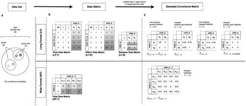
We first clarify the terms data set, data format, data matrices, and (sample) covariance matrices. To this end, we refer to the example in Figure 1. The data set (see Panel A) specifies the data that we collect in a given setting. Relevant information are the sample sizes and the number of observed variables at both levels. At level-2, we have the number of groups g. At level-1, we have the group size n, and the total sample size $N=g·n.$ For means of simplification, we restrict our example to the same observed variables p at both levels. In other words, we only look at level-2 variables that are aggregates of level-1 variables. Models that include the same variable at both levels are often referred to as contextual analysis models (e.g., Boyd & Iversen, 1979; Raudenbush & Bryk, 2002). In our example, we observed two groups (g = 2) with two units each (n = 2), resulting in a total sample size of $N=g·n=4$ units. For every level-1 unit we observed two variables (p = 2), x₁ and x₂, which we aggregate to obtain level-2 variables. The data matrix (see Panel B) specifies the data set in matrix form. It has two dimensions, columns and rows. The dimensions of the data matrix depend on the sample sizes and the number of observed variables, and, importantly, on the data format. We can arrange our data set either in LF or in WF. The data format further determines which sample covariance matrices are estimated. The sample covariance matrix contains the variances and covariances of the observed variables (i.e., of the columns of the respective data matrix). Note that the sample covariance matrix (S) is not always the unbiased population covariance matrix estimator ($\widehat{\mathbf{\Sigma }}$). This is why we refer to the entirety of covariance matrices of the observed variables as covariance matrices (see Panel C). Next we consider the data matrices and covariance matrices more closely. Note that the procedures we present in the following correspond to the multilevel modeling approaches by Muthén (1990, 1994) and Mehta and Neale (2005) and their implementation in lavaan that we investigated in our study, and may not generalize to other approaches.

Figure 1. Representation of data set and (Co)variances. Example data set with number of groups g = 2, group size n = 2, and number of observed variables p = 2. In the WF approach, p is split into n specific-units variables (e.g., $x_{1.2}$ is x₁ for every 2^nd unit in the group). We have coding variables for each unit (ID), units within groups (i), and groups (j). The grey shades indicate different units. κ = condition number. ${\widehat{\mathbf{\Sigma }}}_{\mathit{\text{LF}}-B}$ in lavaan = ${\widehat{\mathbf{\Sigma }}}_{\mathit{\text{LF}}-B}$ with negative variances and related covariances set to 0.

1.1. Long Format: Multilevel Representation of Data Set and (Co)variances

When we arrange the data set in long format (LF), the total raw data matrix (LF-T) has p columns and $N=g·n$ rows. We decompose the total data matrix (LF-T) into the between-group data matrix (LF-B) and the within-group data matrix (LF-W), see the upper part of Panel B of Figure 1, to separate the total (co)variance of each variable(s) into between-group and within-group components. For this, the group means (on level-2) are estimated and subtracted from the value of their respective level-1 units for every observed variable. The group means constitute the data matrix LF-B with p columns and g rows. The deviations from these group means constitute the data matrix LF-W with p columns and $g·n$ rows. Both LF-W and LF-B include all units for every p, resulting in all-units (co)variances³. One sample covariance matrix for each level using LF-W and LF-B is estimated.

The ML estimators for the sample covariance matrices of the two levels, the pooled within-group estimator in Equation (1)(1) $${\mathbf{S}}_{\mathit{\text{LF}}-W}=\frac{1}{N-g}\sum _{j=1}^g\sum _{i=1}^n({\mathbf{X}}_{\mathit{\text{ij}}}-{\overline{\mathbf{X}}}_j){({\mathbf{X}}_{\mathit{\text{ij}}}-{\overline{\mathbf{X}}}_j)}^T,$$(1) and the between-group estimator in Equation (2)(2) $${\mathbf{S}}_{\mathit{\text{LF}}-B}=\frac{n}{g-1}\sum _{j=1}^g({\mathbf{X}}_j-\overline{\mathbf{X}}){({\mathbf{X}}_j-\overline{\mathbf{X}})}^T,$$(2) (Muthén, 1990, 1994), read: (1) $${\mathbf{S}}_{\mathit{\text{LF}}-W}=\frac{1}{N-g}\sum _{j=1}^g\sum _{i=1}^n({\mathbf{X}}_{\mathit{\text{ij}}}-{\overline{\mathbf{X}}}_j){({\mathbf{X}}_{\mathit{\text{ij}}}-{\overline{\mathbf{X}}}_j)}^T,$$(1) (2) $${\mathbf{S}}_{\mathit{\text{LF}}-B}=\frac{n}{g-1}\sum _{j=1}^g({\mathbf{X}}_j-\overline{\mathbf{X}}){({\mathbf{X}}_j-\overline{\mathbf{X}})}^T,$$(2) with $j=1,\dots ,g$ groups and $i=1,\dots ,n$ units per group. ${\mathbf{X}}_{\mathit{\text{ij}}}$ denotes the raw data in LF (i.e., LF-T), ${\overline{\mathbf{X}}}_j$ denotes group mean estimates (i.e., LF-B), $({\mathbf{X}}_{\mathit{\text{ij}}}-{\overline{\mathbf{X}}}_j)$ denotes unit-wise deviations from these group mean estimates (i.e., LF-W), $\overline{\mathbf{X}}$ denotes a row vector with grand mean estimates, and ^T is the matrix transpose.

For the within-group level, the unbiased ML estimator of the population covariance matrix is the pooled within-group sample covariance matrix, ${\mathbf{S}}_{\mathit{\text{LF}}-W}={\widehat{\mathbf{\Sigma }}}_{\mathit{\text{LF}}-W}.$ However, for the between-group level, the unbiased ML estimator of the population covariance matrix is a function of the sample covariance matrices of both levels (Muthén, 1990, 1994): (3) $${\widehat{\mathbf{\Sigma }}}_{\mathit{\text{LF}}-B}=\frac{1}{c}({\mathbf{S}}_{\mathit{\text{LF}}-B}-{\mathbf{S}}_{\mathit{\text{LF}}-W}),$$(3) where c denotes the common group size, and in the case of balanced data, c = n. The $\mathit{\text{cols}}:\mathit{\text{rows}}$ implied biases in the eigenvalues are $p:(g·n)$ for ${\mathbf{S}}_{\mathit{\text{LF}}-W}={\widehat{\mathbf{\Sigma }}}_{\mathit{\text{LF}}-W}$ and $p:g$ for ${\mathbf{S}}_{\mathit{\text{LF}}-B}$ and ${\widehat{\mathbf{\Sigma }}}_{\mathit{\text{LF}}-B}.$ However, note that ${\mathbf{S}}_{\mathit{\text{LF}}-B}$ and ${\widehat{\mathbf{\Sigma }}}_{\mathit{\text{LF}}-B}$ are influenced by more factors than p and g, which we will discuss in the next section, and that in lavaan, negative variances and related covariances in ${\widehat{\mathbf{\Sigma }}}_{\mathit{\text{LF}}-B}$ are set to zero⁴. Thus, the eigenvalues of these LF-B covariance matrices differ from what we would expect from $\mathit{\text{cols}}:\mathit{\text{rows}}$ alone. All LF covariance matrices are shown in the upper part of Panel C of Figure 1.

1.1.1. Why Between-Group Covariance Matrices Have Even More Problems with Unfavorable Matrix Properties

As outlined, LF-B has larger $\mathit{\text{cols}}:\mathit{\text{rows}}$ than LF-W, more specifically, $p:g$ in contrast to $p:(g·n),$ which implies larger bias in the eigenvalues of ${\mathbf{S}}_{\mathit{\text{LF}}-B}$ than of ${\mathbf{S}}_{\mathit{\text{LF}}-W}.$ Hence, non-singularity, non-positive definiteness, and high condition numbers are more likely. However, the eigenvalues of ${\mathbf{S}}_{\mathit{\text{LF}}-B}$ and ${\widehat{\mathbf{\Sigma }}}_{\mathit{\text{LF}}-B}$ are likely not only influenced by the $\mathit{\text{cols}}:\mathit{\text{rows}}$ of LF-B. For example, the probability of being non-positive definite increases not only with increasing p and decreasing g (which links to the $\mathit{\text{cols}}:\mathit{\text{rows}}$) but also with decreasing group sizes n and intraclass correlation⁵ (ICC; Bhargava & Disch, 1982; Hill & Thompson, 1978; Searle et al., 1992). Further, ${\widehat{\mathbf{\Sigma }}}_{\mathit{\text{LF}}-B}$ is estimated as the difference of ${\mathbf{S}}_{\mathit{\text{LF}}-B}$ and ${\mathbf{S}}_{\mathit{\text{LF}}-W},$ see Equation (3)(3) $${\widehat{\mathbf{\Sigma }}}_{\mathit{\text{LF}}-B}=\frac{1}{c}({\mathbf{S}}_{\mathit{\text{LF}}-B}-{\mathbf{S}}_{\mathit{\text{LF}}-W}),$$(3) , and the subtraction often results in a non-positive definite covariance matrix even when both sample covariance matrices are positive definite (Bhargava & Disch, 1982; Hill & Thompson, 1978). Non-positive definiteness indicates zero or negative eigenvalues, which is related to singularity and high condition numbers. In sum, the fact that the occurrence of non-positive definiteness is related to larger p, and smaller g, n, and ICC, suggests that the exact bias term of ${\mathbf{S}}_{\mathit{\text{LF}}-B}$ and ${\widehat{\mathbf{\Sigma }}}_{\mathit{\text{LF}}-B}$ may be different than $p:g.$ We will elaborate more on this assumption shortly.

1.2. Wide Format: Single Level Representation of Data Set and (Co)variances

When we arrange the data set in WF, the total raw data matrix (WF-T) has $p·n$ columns and g rows, see the lower part of Panel B of Figure 1. Here we do not separate the total (co)variance in within- and between-group components. However, each variable p is split into n specific-units variables, or as Mehta and Neale (2005, p.1) put it, “people [n] are variables too.” One sample covariance matrix is estimated from WF-T.

We estimate the sample covariance matrix with the estimator for single level data. The single level represented two-level sample covariance matrix with specific-units (co)variances reads: (4) $${\mathbf{S}}_{\mathit{\text{WF}}-T}=\frac{1}{g}\sum _{j=1}^g(\mathbf{X}.{\mathbf{i}}_j-\overline{\mathbf{X}.\mathbf{i}}){(\mathbf{X}.{\mathbf{i}}_j-\overline{\mathbf{X}.\mathbf{i}})}^T,$$(4) where $\mathbf{X}.\mathbf{i}$ denotes the raw data in WF (i.e., WF-T) and $\overline{\mathbf{X}.\mathbf{i}}$ denotes a row vector with grand mean estimates. ${\mathbf{S}}_{\mathit{\text{WF}}-T}$ is the so-called biased ML estimator⁶ for ${\mathbf{\Sigma }}_{\mathit{\text{WF}}-T}.$ The $\mathit{\text{cols}}:\mathit{\text{rows}}$ implied bias in the eigenvalues of ${\mathbf{S}}_{\mathit{\text{WF}}-T}$ is $(p·n):g.$ We see ${\mathbf{S}}_{\mathit{\text{WF}}-T}$ in the lower part of Panel C of Figure 1.

1.3. Summary and Comparison

All LF and WF covariance matrices are estimated by ML. The $\mathit{\text{cols}}:\mathit{\text{rows}}$ of LF-W, LF-B, and WF-T, are $p:(g·n),p:g,$ and $(p·n):g.$ Thus, the order of the magnitude of $\mathit{\text{cols}}:\mathit{\text{rows}}$ is LF-W < LF-B < WF-T. However, it is unclear whether the $\mathit{\text{cols}}:\mathit{\text{rows}}$ bias in sample eigenvalues in single level settings is directly applicable to multilevel settings. As we pointed out earlier, evidence suggests that the between-group covariance matrices are not only influenced by the $\mathit{\text{cols}}:\mathit{\text{rows}}$ of LF-B. However, no study investigated the exact bias term of the eigenvalues of LF and WF covariance matrices before. Within the scope of this study, we are not interested in the exact term of the bias. Rather we use $\mathit{\text{cols}}:\mathit{\text{rows}}$ as a proxy of the eigenvalue bias, because we assume that it is the main influence on the bias. Let us support this assumption by looking at the other matrix properties of the LF and WF covariance matrices, which are shown in Panel C of Figure 1. ${\widehat{\mathbf{\Sigma }}}_{\mathit{\text{LF}}-W}$ is non-singular, positive definite, and has a small condition number. We see that ${\widehat{\mathbf{\Sigma }}}_{\mathit{\text{LF}}-B}$ has only negative variances. Thus, in lavaan all elements are set to zero which results in a singular, positive-semi definite matrix with an infinite condition number. ${\widehat{\mathbf{\Sigma }}}_{\mathit{\text{WF}}-T}$ is singular, indefinite, and has an infinite condition number. Note that negative variances in ${\widehat{\mathbf{\Sigma }}}_{\mathit{\text{WF}}-T}$ are kept which might contribute to inadmissible values (“Heywood cases”). In sum, the LF covariance matrices are assumed to have a smaller eigenvalue bias than the WF covariance matrix.

2. How Data Format Influences Multilevel SEM Approaches

It has been shown that ML estimation in multilevel SEM (Muthén, 1990, 1994) is analytically and in certain settings empirically equivalent to single level restricted confirmatory factor analysis (CFA) models (Barendse & Rosseel, 2020; Mehta & Neale, 2005). The multilevel SEM approach uses the data matrix in LF. The single level approach uses the data matrix in WF. More specifically, Mehta and Neale (2005) demonstrated analytical equivalence of the LF and WF approach for continuous, unbalanced data with full information ML (FIML) estimation, and provided an empirical example which used the WF approach (in Mplus). Barendse and Rosseel (2020) demonstrated empirical equivalence of the LF and WF approach for discrete, balanced and unbalanced data with marginal ML (MML) and pairwise ML (PML) estimation in a Monte Carlo study (in lavaan and Mplus). With very small group sizes n = 3 (but large g) the WF approach even resulted in somewhat less biased parameter estimates. However, all empirical data sets contained only small p and n, and large g (and thus large N), which resulted in $\mathit{\text{cols}}\ll \mathit{\text{rows}}$ in all involved data matrices, and no significant differences in the $\mathit{\text{cols}}:\mathit{\text{rows}}$ of the data matrices of both formats. In contrast, different $\mathit{\text{cols}}:\mathit{\text{rows}}$ imply different magnitudes of eigenvalue bias. Thus, data sets that result in strongly different $\mathit{\text{cols}}:\mathit{\text{rows}}$ in both formats imply differences in convergence and estimation accuracy. In lavaan, the multilevel SEM (LF) approach is yet implemented only for continuous data. Thus, we restricted our analysis to continuous, balanced data and standard normal-theory ML estimation for both the LF and WF approach⁷. We do not want to go into detail about the model estimation and fitting functions here. The interested reader is referred to Mehta and Neale (2005). Instead, we want to underline how the data format influences the modeling approaches, more specifically, the model specifications and minimum data set requirements.

2.1. Model Specification

Whereas the same multilevel model can be estimated in the LF and WF approaches, their model specifications differ. For reasons of simplicity, we only consider so called “intercept-only models” (e.g., Hox et al., 2017; Raudenbush & Bryk, 2002) of all-units (co)variances. In other words, we model the p variables covariance structure for the within- and between-group level which is equivalent to the LF covariance matrices. In the LF approach, we have the same model specification at each level. The (co)variances at both levels are modeled as (co)variances of the p observed variables (from ${\widehat{\mathbf{\Sigma }}}_{\mathit{\text{LF}}-W}$ and ${\widehat{\mathbf{\Sigma }}}_{\mathit{\text{LF}}-B},$ respectively). In the WF approach, the model specification differs at both levels. In contrast to the LF approach, all parameters are modeled as (co)variances of latent factors of the observed p × n specific-units variables (from ${\widehat{\mathbf{\Sigma }}}_{\mathit{\text{WF}}-T}$). 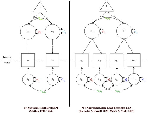To estimate the all-units (co)variances, the between-group parameters are modeled as common factors, with factor loadings set to 1, and the within-group parameters are modeled as unique factors, with equality constraints added to (co)variances of the unique factors of the same variable p. Note that with the equality constraints, homoscedasticity of specific-units variables is modeled. Figure 2 depicts the model specifications for a contextual intercept-only model for both approaches, using the earlier example data set. Note that in both approaches, the mean structure at the between-group level has to be included in order to discern the total (co)variance into within- and between-group parts. In the “genuine” multilevel approach (LF), this is done implicitly. In the restricted single level CFA approach (WF), we have to add it. Example R code for the specification and estimation of both models is presented in the Online Supplemental Material.

Figure 2. Example model specification in the LF and WF approach for a contextual intercept-only model. Example data set with group size n = 2, and number of observed variables p = 2. In the WF approach, p is split into n specific-units variables (e.g., $x_{1.2}$ is x₁ for every 2^nd unit in the group; see also Figure 1), and identical parameter labels indicate equality constraints in the model. Across both approaches, the same parameters have the same color. Across both levels, matching parameters have similar color. Affiliation of parameters to the between- and within-group level is indicated by location above and below the dashed line.

2.2. Software Requirements

We want to consider two requirements of lavaan because they are connected to the (sample) covariance matrices and their matrix properties. The first requirement concerns both approaches; the second concerns only the LF approach.

2.2.1. Minimum Data Set

One requirement of lavaan is that the data matrices we give as input, LF-T and WF-T, respectively, need to have $\mathit{\text{cols}}\le \mathit{\text{rows}}.$ This requirement is likely based in the fact that sample covariance matrices have undesirable matrix properties in these settings. For example, when cols > rows, at least one sample eigenvalue becomes zero and the sample covariance matrix turns singular (e.g., Duncan et al., 1997; Gorsuch, 1983; Wothke, 1993). Whereas the ML estimators in the LF and WF approach does not require the covariance matrices to be non-singular (i.e., invertible), singular matrices are non-positive definite and result in an infinite condition number, which might have a negative impact on convergence and estimation accuracy. Due to the different $\mathit{\text{cols}}:\mathit{\text{rows}}$ of LF-T and WF-T, $p:(g·n)$ and $(p·n):g,$ the minimum data set requirements for both approaches differ. Two points are noteworthy here. Firstly, larger group sizes n are advantageous for LF-T, but disadvantageous for WF-T. Secondly, there are settings where we can only use the LF approach because $p<(g·n)$ (in LF-T) is more easily satisfied than $(p·n)<g$ (in WF-T). Our example data set with g = 2, n = 2, and p = 2, would result in $2:4$ in LF-T and $4:2$ in WF-T. Thus, we could only use the LF approach to analyze it. Note that the $\mathit{\text{cols}}\le \mathit{\text{rows}}$ requirement generally supports the importance of considering $\mathit{\text{cols}}:\mathit{\text{rows}}.$

2.2.2. Definiteness of ${\widehat{\mathbf{\Sigma }}}_{\mathit{\text{LF}}-B}$

In the LF approach, there is one further requirement. Model estimation with the quasi-Newton algorithm (the default) fails with an error when ${\widehat{\mathbf{\Sigma }}}_{\mathit{\text{LF}}-B}$ is negative definite (i.e., has only negative eigenvalues; see e.g., Rosseel, 2018). This might be the reason why lavaan sets negative variances and related covariances in ${\widehat{\mathbf{\Sigma }}}_{\mathit{\text{LF}}-B}$ to 0, because this seems to prevent that all eigenvalues are negative. Thus, we do not have to worry about this requirement, but keep in mind, that ${\widehat{\mathbf{\Sigma }}}_{\mathit{\text{LF}}-B}$ can be altered.

3. This Study

The aim of this study is to investigate the equivalent of the $p:N$ ($\mathit{\text{cols}}:\mathit{\text{rows}}$) effect on convergence and estimation accuracy in multilevel SEM. To this end, we scrutinize the LF and WF approach in settings which result in different $\mathit{\text{cols}}:\mathit{\text{rows}}$ of the data matrices of both data formats. We use $\mathit{\text{cols}}:\mathit{\text{rows}}$ as a proxy of the eigenvalue bias of the LF and WF covariance matrices. Two (intertwined) effects are considered: (a) the effect of the data format, with its inherently different $\mathit{\text{cols}}:\mathit{\text{rows}},$ and (b) the effect of $\mathit{\text{cols}}:\mathit{\text{rows}}$ in each data format. By investigating (a) the effect of the data format, we want to learn which data format (and related approach) to prefer in a given setting. The same setting results in inherently different $\mathit{\text{cols}}:\mathit{\text{rows}}$ in the data matrices of both approaches. For example, the setting g = 10, n = 2, and p = 2 results in $2:20$ in LF-W, $2:10$ in LF-B, and $4:10$ in WF-T. Unless all data matrices have $\mathit{\text{cols}}\ll \mathit{\text{rows}},$ we assume that the LF approach, which has inherently smaller $\mathit{\text{cols}}:\mathit{\text{rows}}$ in its data matrices, outperforms the WF approach. We are also interested in (b) the effect of $\mathit{\text{cols}}:\mathit{\text{rows}}$ in each data format, to gather insight into optimal study design. On that account, different settings that result in the same $\mathit{\text{cols}}:\mathit{\text{rows}}$ in both data formats are investigated. Out of the multiple data matrices in LF, we focus on LF-B. We do so because LF-B does not have to satisfy cols < rows in lavaan, which implies more possible variation in $\mathit{\text{cols}}:\mathit{\text{rows}},$ and thus has the largest (i.e., most problematic) $\mathit{\text{cols}}:\mathit{\text{rows}}$ among the data matrices in LF. To continue the example, to have $4:10$ in LF-B (like in WF-T), we need another setting, for example where p = 4 (and g = 10 and n = 2 stay the same).

3.1. Method

In the following, we outline the data generation and evaluation criteria of the Monte Carlo study. As pointed out earlier, we only considered intercept-only models at the within- and between-group level. As a consequence, the data-generating model equals the data analysis model. All computations were performed on an AMD Ryzen Threadripper PRO 3975WX 32-cores (3.50 GHz) CPU on a Windows 10 (Version 20H2) platform. Data generation and analysis was conducted using R version 4.3.1 (R Core Team, 2023)⁸. The R code for data, analysis, tables, and figures is available at https://github.com/demianJK/LF_WF_SEM.

3.1.1. Data Generation

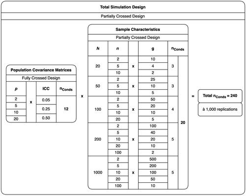
For the data generation, we drew from a multivariate normal distribution with population means fixed to zero and varying population covariance matrices and sample characteristics. Data generation was done in LF and separately for level-1 and level-2 data (see also example LF model in Figure 2). With respect to the population covariance matrices, we varied the number of observed variables p and the ICC. The range of the ICC was informed by common values in the social sciences (Gulliford et al., 1999). The total variance of each observed variable, ${\sigma }_B^2+{\sigma }_W^2,$ was constrained to be 1. Hence, ${\sigma }_B^2=\mathit{\text{ICC}}$ and ${\sigma }_W^2=1-{\sigma }_B^2.$ The variances for each level were then used to compute the covariances, respectively, with a fixed correlation of .30. Note that these variances and covariances are also the parameters in our intercept-only models. Applying a fully-crossed design for p and the ICC, we arrived at 12 different population conditions. With respect to the sample characteristics, we varied the total sample size N, the numbers of units per group n, and the number of groups g. We first set N and n, computed $g=N/n$ and then excluded all conditions where $N\ge n,$ g < 2, and where g was not an integer. Applying the described partially crossed design for N, n, and g, we arrived at 20 different sample conditions. Note that we chose the variations of p, n, and g to create conditions where LF-T has $\mathit{\text{cols}}\le \mathit{\text{rows}}$ (and thus, LF-B and WF-T have cols > rows, cols = rows, or cols < rows). We have done this because of the $\mathit{\text{cols}}\le \mathit{\text{rows}}$ requirement of lavaan for LF-T and WF-T. When LF-T has cols > rows, then WF-T has cols > rows, too, and neither approach could be applied. Moreover, we did this to investigate whether the LF approach leads to good results in settings where it is applicable but the WF approach is not (i.e., LF-T has $\mathit{\text{cols}}\le \mathit{\text{rows}},$ but WF-T has cols > rows). Finally, we partially crossed the population and sample conditions and arrived at a total of 240 simulation conditions. For each condition, we simulated 1000 data sets. The complete simulation design is shown in Figure 3.

Figure 3. Simulation design.

3.1.2. Evaluation Criteria

To assess model performance, we included convergence rate, and for estimation accuracy, relative root mean squared error (RMSE), relative bias, and relative variance⁹. The RMSE assesses the overall accuracy of an estimator. It is defined as the square root of the mean of the squared differences between the estimates and the population value. Bias is a measure to assess the extent with which an estimator targets the population value. It is defined as the mean of the differences between the estimates and the population value. Variance is a measure of the efficiency of an estimator. It is defined as the mean of the differences between the estimates and the mean of all estimates. We used the relative versions of these parameters dividing them by the respective population value (which is determined by the ICC). We further multiplied them by 100 to arrive at percentages. We did this to investigate potential differences in accuracy, bias, and efficiency with respect to the ICC. For example, when RMSE = 0.1 for both $\theta =\mathit{\text{ICC}}=0.5$ and $\theta =\mathit{\text{ICC}}=0.1,$ this mounts to relative RMSE of 20% and 100%, respectively, which suggests that the estimation of the smaller ICC is less accurate. Note that we only consider estimation accuracy of (co)variances but not of means of the intercept-only models.

3.2. Results

In the following, we summarize the results of (a) the effect of the data format, and (b) the effect of $\mathit{\text{cols}}:\mathit{\text{rows}}$ on convergence and estimation accuracy criteria in each data format. For this purpose, we plotted the results of the Monte Carlo study aggregated (a) by the sample size at level-2, the number of groups g (same data set, different data formats), and (b) by $\mathit{\text{cols}}:\mathit{\text{rows}}$ of LF-B and WF-T (different data sets, same data format). Out of the sample sizes at the two levels, level-1 group size n, and level-2 number of groups g, we decided to plot the latter because it equals the number of rows (i.e., observations) in both LF-B and WF-T. Table 1 shows descriptive statistics of the convergence and estimation accuracy criteria. Note that for the latter, we used only simulation conditions that resulted in 100% convergence in both approaches to minimize differences in Monte Carlo error in both approaches and thus, facilitate comparison of both approaches. An overview of the results of the simulation study clustered by the factors of the simulation design (i.e., 240 simulation conditions for each approach) can be found in Figure 2 in the Online Supplemental Material.

Table 1. Descriptive statistics of the model performance criteria.

Criterion	M	SD	Median	Min	Max
Convergence rate^a	49.28	49.33	49.25	0.00	100.00
Relative RMSE^b	84.83	101.44	47.76	14.04	571.09
Relative bias^b	−4.12	12.42	−1.27	−105.16	5.04
Relative variance^b	10.36	20.33	3.10	0.48	144.17

Unit for all criteria is %.

^aN = 480 (all simulation conditions for both approaches).

^bN = 156 (all simulation conditions that converged 100% in both approaches).

3.2.1. The Effect of Data Format

3.2.1.1. Convergence

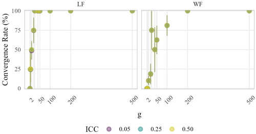
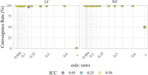
In Figure 4, convergence rates aggregated by sample size at level-2 g are depicted. It is evident that with increasing g, average convergence rates increased with a seemingly logarithmic trend in the LF and WF approach. Nevertheless, there was an effect of data format on convergence, as the LF approach was more likely to converge in small and moderate sample sizes. For instance, the average convergence rate in g = 100 was 100% in the LF approach, and 80% in the WF approach. Further, for the WF approach, we see that the convergence trend was non-monotonous with g. Whereas g = 25 had an average convergence rate of 75%, g = 40 and g = 50 had lower ones. The non-monotonous trend of the WF approach suggests that other terms than g might also be relevant for convergence. We will scrutinize this matter in the following section when investigating the $\mathit{\text{cols}}:\mathit{\text{rows}}$ effects.

Figure 4. Convergence aggregated by sample size at level-2. Points indicate means; lines indicate means ± standard errors (i.e., variability across simulation conditions). The sample size at level-2 g corresponds to the rows of both LF-B and WF-T.

3.2.1.2. Estimation Accuracy

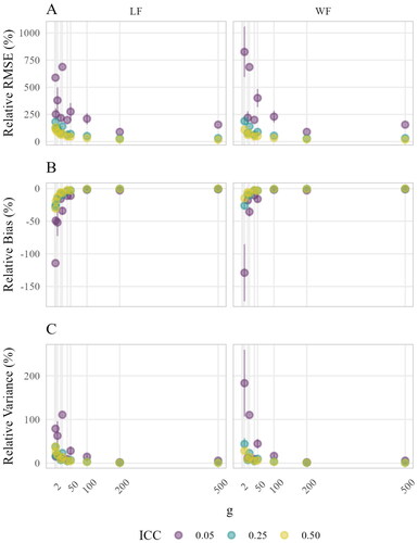
Results for the estimation accuracy of between-group parameters are shown in Figure 5. The relative RMSE (Panel A), relative bias (Panel B), and relative variance (Panel C) decreased with larger numbers of groups g in a very similar fashion for both approaches. Slight differences were only present for settings with small g and small ICC where variability across simulation conditions was large. Overall, this suggests that there was no substantial effect of the data format on estimation accuracy of between-group level parameters. However, the findings revealed a connection between the estimation accuracy of between-group level parameters and the magnitude of the ICC. Specifically, the smaller the ICC, the more inaccurate, biased, and inefficient were the between-group parameters. Besides main effects of g and ICC, the results further imply an interaction effect. The least accurate, most biased, and inefficient results were obtained in settings with small g and small ICC.

Figure 5. Estimation accuracy of between-group parameters aggregated by sample size at level-2. Points indicate means; lines indicate means ± standard errors (i.e., variability across simulation conditions). The sample size at level-2 g corresponds to the rows of both LF-B and WF-T.

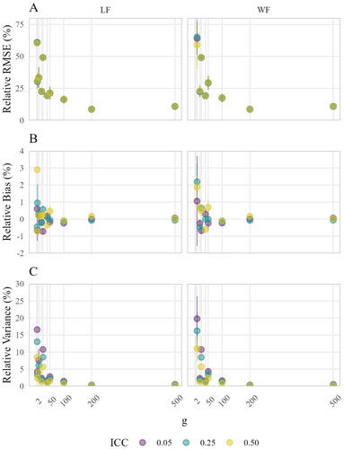
Similar patterns have been found for the estimation accuracy of the within-group parameters that are depicted in Figure 6. However, in contrast to the between-group parameters, an effect of the ICC was only present for the relative variance, as was an interaction effect of g and ICC. Furthermore, the within-group parameters were overall more accurate, less biased, and more efficient than the between-group parameters.

Figure 6. Estimation accuracy of within-group parameters aggregated by sample size at level-2. Points indicate means; lines indicate means ± standard errors (i.e., variability across simulation conditions). The sample size at level-2 g corresponds to the rows of both LF-B and WF-T.

3.2.1.3. Summary

Our findings suggest that there was an effect of data format on convergence, but not on estimation accuracy, despite the different $\mathit{\text{cols}}:\mathit{\text{rows}}$ (and implied magnitudes of eigenvalue biases) in both approaches. Further, we found an interaction effect of g, ICC, and parameter level on estimation accuracy. More specifically, the least accurate, most biased, and inefficient parameter estimates were obtained in samples with small numbers of groups, small ICC values, and at the between-group level.

3.2.2. The Effect of Cols : Rows in Each Data Format

3.2.2.1. Convergence

In Figure 7, convergence rates aggregated by $\mathit{\text{cols}}:\mathit{\text{rows}}$ of LF-B and WF-T, $p:g$ and $(p·n):g,$ are shown. For cols < rows, both approaches led to average convergence rates of $\approx 100\%.$ For cols = rows, however, results for both approaches differed. In LF, this always led to non-convergence. In WF, half of the models converged. For the LF approach, this extends the minimum data set requirements given by lavaan and informs about optimal study design. We require cols < rows in the input data matrix LF-T ($p<(g·n)$) to use lavaan, and our results suggest that we additionally need to satisfy cols < rows in LF-B (p < g) to get a converging model in the LF approach. In other words, we have to design our study in such a way that the number of level-2 variables is smaller than the number of groups. The reason why p < g is required might be connected to the eigenvalue bias in ${\widehat{\mathbf{\Sigma }}}_{\mathit{\text{LF}}-B},$ which might have been non-negligible when cols = rows¹⁰. However, we cannot confirm that because we used $\mathit{\text{cols}}:\mathit{\text{rows}}$ only as a proxy of the eigenvalue bias. Comparing convergence rates aggregated by $\mathit{\text{cols}}:\mathit{\text{rows}}$ and aggregated by sample size at level-2 (i.e., rows; see Figure 4), it can be seen that the former exhibited smaller variability and thus, gave more reliable information on convergence. It further suggests that the effect of data format on convergence was attributable to the differences in $\mathit{\text{cols}}:\mathit{\text{rows}}$ in both approaches.

Figure 7. Convergence aggregated by $\mathit{\text{Cols}}:\mathit{\text{Rows}}.$ Points indicate means; lines indicate means ± standard errors (i.e., variability across simulation conditions). The $\mathit{\text{cols}}:\mathit{\text{rows}}$ of LF-B and WF-T, $p:g$ and $(p·n):g,$ are depicted.

3.2.2.2. Estimation Accuracy

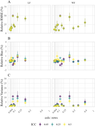
We saw in the last section that there was no noticeable effect of data format on estimation accuracy. Put differently, the estimation accuracy in both approaches was very similar for a given number of groups g (i.e., rows of LF-B and WF-T) despite different cols, and thus, $\mathit{\text{cols}}:\mathit{\text{rows}}$ of LF-B and WF-T. This suggests that there must have been different effects for $\mathit{\text{cols}}:\mathit{\text{rows}}$ in each data format. In Figure 8, the relative RMSE (Panel A), relative bias (Panel B), and relative variance (Panel C) by the $\mathit{\text{cols}}:\mathit{\text{rows}}$ in each data format are shown. We indeed see that the $\mathit{\text{cols}}:\mathit{\text{rows}}$ effect is less steep in the WF approach. For example, similar relative RMSE, relative bias, and relative variance where obtained with an $\mathit{\text{cols}}:\mathit{\text{rows}}$ of 0.2 in LF-B in the LF approach and 0.4 in WF-T in the WF approach. Within each data format, larger $\mathit{\text{cols}}:\mathit{\text{rows}}$ resulted in larger relative RMSE, relative bias, and relative variance. Further, there was an interaction with the ICC. Larger $\mathit{\text{cols}}:\mathit{\text{rows}}$ and smaller ICC values led to more inaccurate, biased, and inefficient estimation, with the most problematic results in settings with large $\mathit{\text{cols}}:\mathit{\text{rows}}$ and small ICC values. To continue the example from above, a $\mathit{\text{cols}}:\mathit{\text{rows}}$ of 0.2 in LF-B in combination with the smallest ICC 0.05 yielded approximately a six times higher relative RMSE than large ICC values of 0.50 in the LF approach. Note however, that these $\mathit{\text{cols}}:\mathit{\text{rows}}$ effects, and interaction effects of $\mathit{\text{cols}}:\mathit{\text{rows}}$ and ICC were not strictly monotonous. We will take up the issue in the discussion.

For the estimation accuracy of the within-group parameters, which is depicted in Figure 9, there was a slightly increasing trend in relative RMSE (Panel A) and relative variance (Panel C) with increasing $\mathit{\text{cols}}:\mathit{\text{rows}}.$ For the relative bias (Panel B), there was no systematic trend. In addition, the relative variance showed small effects of the ICC. Smaller ICC resulted in somewhat larger relative variance. Overall, as for the between-group parameters, the $\mathit{\text{cols}}:\mathit{\text{rows}}$ effect of the WF approach was less steep. Compared to the between-group parameters, the effects of $\mathit{\text{cols}}:\mathit{\text{rows}}$ and the ICC on the estimation accuracy of the within-group parameters were very small.

Figure 8. Estimation accuracy of between-group parameters aggregated by $\mathit{\text{Cols}}:\mathit{\text{Rows}}.$ Points indicate means; lines indicate means ± standard errors (i.e., variability across simulation conditions). The $\mathit{\text{cols}}:\mathit{\text{rows}}$ of LF-B and WF-T, $p:g$ and $(p·n):g,$ are depicted.

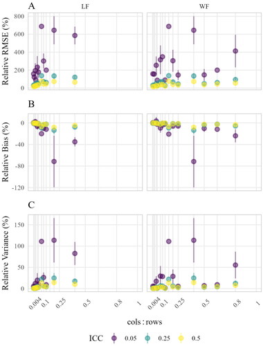
Figure 9. Estimation accuracy of within-group parameters aggregated by $\mathit{\text{Cols}}:\mathit{\text{Rows}}.$ Points indicate means; lines indicate means ± standard errors (i.e., variability across simulation conditions). The $\mathit{\text{cols}}:\mathit{\text{rows}}$ of LF-B and WF-T, $p:g$ and $(p·n):g,$ are depicted.

3.2.2.3. Summary

The results showed that there were differential effects of $\mathit{\text{cols}}:\mathit{\text{rows}}$ on convergence and estimation accuracy in both data formats (approaches). With regard to convergence, we found that cols < rows in LF-B (p < g) and $\mathit{\text{cols}}\le \mathit{\text{rows}}$ in WF-T ($(p·n)\le g$) had to be satisfied which expands the minimum data set requirements of lavaan. For estimation accuracy, the effect in the WF approach was less strong. For both approaches, increasing $\mathit{\text{cols}}:\mathit{\text{rows}}$ and having a smaller ICC was detrimental. These effects were more pronounced for the between-group parameters and smaller ICC values.

4. Discussion

One can arrange a two-level data set in two different data formats, LF and WF. In the two data formats, the involved data matrices, have inherently different $\mathit{\text{cols}}:\mathit{\text{rows}}.$ The $\mathit{\text{cols}}:\mathit{\text{rows}}$ is the $p:N$ equivalent, which depends on g, n, and p in multilevel settings, and implies a magnitude of bias in the sample eigenvalues. For both data formats, SEM approaches to estimate multilevel models with standard ML exist. Past research has provided evidence for analytical and empirical equivalence in settings with large samples sizes at level-2 where $\mathit{\text{cols}}\ll \mathit{\text{rows}}$ in all data matrices, and thus, the assumed bias in eigenvalues was negligibly small. Using a Monte Carlo study, we included settings with small sample sizes at level-2 where $\mathit{\text{cols}}:\mathit{\text{rows}}$ differs in all data matrices. We investigated the effect of the data format (with the same data set in different data formats), and the effects of $\mathit{\text{cols}}:\mathit{\text{rows}}$ (with different data sets in the same data format).

Regarding the effect of the data format, we found only an effect on convergence. In particular, the LF approach with its inherently smaller $\mathit{\text{cols}}:\mathit{\text{rows}}$ was more likely to converge. The estimation accuracy of both approaches did not differ substantially by the choice of the data format. Thus, the results of our study extend the evidence of the empirical equivalence of the LF and WF approaches to settings where both the sample size at level-1 n, and the sample size at level-2 g, are small.

Regarding the $\mathit{\text{cols}}:\mathit{\text{rows}},$ we found differential effects on convergence and estimation accuracy in both data formats (approaches). Concerning the former, the LF approach requires that the number of variables is smaller than the number of groups (p < g), whereas the WF approach requires that the number of variables multiplied by group size is smaller than or equal to the number of groups ($(p·n)<g;$ which is equivalent to the lavaan requirement). $\mathit{\text{Cols}}:\mathit{\text{rows}}$ (number of observed variables to sample size at level-2) includes more information than rows alone (sample size at level-2). It informs us about minimum requirements on study design, and which data format (approach) to use for converging models.

In accordance with the effect of data format, we found differential $\mathit{\text{cols}}:\mathit{\text{rows}}$ effects on estimation accuracy. Within each data format (approach), smaller $\mathit{\text{cols}}:\mathit{\text{rows}}$ resulted in models that yield more accurate, less biased, and more efficient parameter estimates. However, the WF approach had a less steep effect. Thus, the difference in cols, and thus, in $\mathit{\text{cols}}:\mathit{\text{rows}},$ in WF-T compared to LF-B (by the factor n) was not, as expected, detrimental for the estimation accuracy. Instead, the factor n was likely responsible for the less steep effect. Apparently, n appears to simply operate distinctly in both data formats (approaches). In the LF approach, the sample size at level-1 n influences the accuracy of the first and second-order moments at level-2. In the WF approach, the sample size at level-1 n (together with p) determines the number of “observed variables”, but also the number of equality constrains between related model parameters. Having more relations between “observed variables” with equality constrains similarly yields more accurate estimates. In sum, we assumed an effect of data format on estimation accuracy, based on the same $\mathit{\text{cols}}:\mathit{\text{rows}}$ effect on estimation accuracy in both data formats (approaches). However, we found no effect of data format on estimation accuracy, but different $\mathit{\text{cols}}:\mathit{\text{rows}}$ effects on estimation accuracy in both data formats (approaches).

Besides the main effects of data format and $\mathit{\text{cols}}:\mathit{\text{rows}},$ we found further noteworthy effects. Most notable is the interaction between g (or $\mathit{\text{cols}}:\mathit{\text{rows}}$) and magnitude of the ICC and parameter level on estimation accuracy. In particular, the smaller g, or the larger the $\mathit{\text{cols}}:\mathit{\text{rows}},$ and the smaller the ICC values, the more inaccurate, biased, and inefficient are the between-group parameters. Again, these findings reveal valuable insight into optimal study design. When between-group parameters are of interest, and prior studies found marginal ICC values, then future studies should have relatively large g (or $\mathit{\text{cols}}:\mathit{\text{rows}}$).

4.1. Limitations and Directions for Future Research

Firstly, we used the $\mathit{\text{cols}}:\mathit{\text{rows}}$ of a data matrix only as a proxy of the eigenvalue bias of the LF and WF covariance matrices. Our findings showed that within each data format, larger $\mathit{\text{cols}}:\mathit{\text{rows}}$ resulted in lower convergence rates, and less accurate between-group parameter estimates in both approaches, which suggests that eigenvalue biases might have increased with increasing $\mathit{\text{cols}}:\mathit{\text{rows}}.$ However, we did not investigate the exact term of the eigenvalue biases. For example, as pointed out earlier, when level-2 variables are aggregates of level-1 variables, the matrix properties of ${\widehat{\mathbf{\Sigma }}}_{\mathit{\text{LF}}-B}$ are not only influenced by p and g (which constitute $\mathit{\text{cols}}:\mathit{\text{rows}}$), but by n and the ICC (Bhargava & Disch, 1982; Hill & Thompson, 1978; Searle et al., 1992). This suggests that the bias term of its eigenvalues is influenced by these factors. Further, the effect of $\mathit{\text{cols}}:\mathit{\text{rows}}$ on convergence and estimation accuracy was different for the LF and WF approach. This might be related to different eigenvalue biases. On the other hand, it could suggest that eigenvalue biases exert minor influence on convergence and estimation accuracy. Future research could investigate the exact term of the eigenvalue biases of LF and WF covariance matrices, and whether the difference in eigenvalue biases explains the difference in convergence and estimation accuracy.

Secondly, because our study was the first to investigate the $p:N$ ($\mathit{\text{cols}}:\mathit{\text{rows}}$) equivalent within multilevel SEM, we included only simple intercept-only models. The influence in more complex models remains to be investigated. For example, it has been shown that in measurement models, convergence rates decreases with smaller numbers of indicators per factor, and smaller magnitude of factor loadings and factor correlations (J. C. Anderson & Gerbing, 1984; Boomsma, 1985; Jöreskog & Sörbom, 1984). Further, factor correlations are depended on correlations of indicators (i.e., observed variables), which implies that larger correlations of observed variables are desirable. In our study, correlations of all observed variables were fixed to 0.3, and covariances of observed variables were computed by the correlation and the respective variances. Differences in covariances did not show any influence on convergence. However, covariances (correlations) of observed variables have a bivariate nature, whereas factor correlations have a multivariate nature. It would be interesting to investigate how eigenvalue bias influences convergence and estimation accuracy in factor models. Further, level-2 predictors might be examined. We included only level-2 variables that are aggregates of level-1 variables. In other words, we investigated contextual analysis models. With level-2 predictors, the importance of larger n for more accurate between parameters could be smaller. The eigenvalue bias term of between-group covariance matrices of predictor variables is assumed to differ from those of between-group covariance matrices of level-1 aggregates. In sum, future research should investigate the influence of the eigenvalue bias in more complex multilevel SEM models with measurement models and level-2 predictors.

Thirdly, future research could investigate whether improving the eigenvalue structure of LF and WF covariance matrices can improve performance. In single level settings, it has been shown that improving the eigenvalues of the sample covariance matrix can result in increased convergence rates and more accurate model estimates (e.g., Kamada & Kano, 2012; Kamada et al., 2014; Yuan & Bentler, 2017; Yuan & Chan, 2008; Yuan et al., 2011). In multilevel settings, it has been shown that improving the eigenvalues of the model-implied between-group matrix results in more accurate between-group parameters (e.g., Chung et al., 2015; McNeish, 2016; Zitzmann, 2018). It seems promising to investigate improving the eigenvalues of the LF and WF covariance matrices, more specifically, ${\widehat{\mathbf{\Sigma }}}_{\mathit{\text{LF}}-B}$ in the LF approach and ${\widehat{\mathbf{\Sigma }}}_{\mathit{\text{WF}}-T}$ in the WF approach, and whether this could increase the accuracy of between-group parameters.

Fourthly, future studies could examine the effect of the ICC on the bias of the between-group parameters more closely. First, the evidence for its existence is mixed. Whereas some studies found no effect (e.g., Hox et al., 2010; McNeish & Stapleton, 2016; Meuleman & Billiet, 2009; Stegmueller, 2013), other studies, ours included, found that a smaller ICC leads to increased bias (e.g., Hox & Maas, 2001; Lüdtke et al., 2008, 2011; Muthen & Satorra, 1995; Zitzmann et al., 2015). Second, within the studies that found an effect, the direction of the bias differs. Most studies found a downward bias. However, the bias was mostly aggregated over parameters of different types. Hox and Maas (2001) classified them by type and found upward bias in variances and downward bias in factor loadings. Further, the type of parameter also depends on the modeling approach. Lüdtke et al. (2011) compared manifest and latent approaches and found that only the approach who had latent variables at both levels resulted in upward bias. In our study, both approaches incorporated latent variables at both levels, and both exhibited a downward bias. However, we did not distinguish between different types of parameters. Future research could explore how the presence and direction of an ICC effect on the bias of between-group parameters may vary depending on the parameter type.

4.2. Conclusion

Our study has demonstrated two important main results. First, data format influences convergence but not estimation accuracy. Second, the rows and $\mathit{\text{cols}}:\mathit{\text{rows}}$ of data matrices, which varies when conducting multilevel analysis in long versus wide format, along with the ICC are critical factors influencing the convergence and estimation accuracy of multilevel SEM approaches. To conclude with some literary advice: We aim for convergence all along, with accuracy nothing going wrong, especially if the ICCs are not strong, our data matrices should be comparatively long.

Disclosure statement

The authors report there are no competing interests to declare.

Notes

1 Note that Hayashi et al. (2018) pointed out that when p is negligibly small relative to N, the magnitude of the bias is $1:N.$ However, when p is not negligibly small relative to N, which is commonly the case, the magnitude of the bias is $p:N.$

2 Note that a large strain of research in large p, small N settings focused on the “model size” effect, which has been conceptualized in many different ways: as the effect of the number of observed variables p (Shi et al., 2018, 2019), the number of freely estimated parameters q (Shi et al., 2018), the number of participants per (freely estimated) parameter $N:q$ (Herzog et al., 2007; Jackson, 2001, 2003), or a function of both p and q, the degrees of freedom df (Herzog et al., 2007; Shi et al., 2018). Because it has not been conceptualized as $p:N,$ we do not go into detail about the model size effect here.

3 Barendse and Rosseel (2020) introduced the term unit-specific with regards to the WF covariance matrix. To avoid confusion with within-group effects and make the difference between LF and WF more succinct, we use the terms specific-units (co)variances for the WF covariance matrix, and all-units (co)variances for the LF covariance matrices instead.

4 We found no information on this procedure in the reference manual or presentations but discovered it by chance. The potential reason is discussed later.

5 Hox et al. (2017) define the ICC as amount of between-group variance out of the total variance (i.e., sum of between- and within-group variance), ${\sigma }_B^2/({\sigma }_B^2+{\sigma }_W^2).$

6 In the unbiased ML estimator, the denominator would be $g-1.$ However, we focus on the biased estimator because it is the default in lavaan (see Rosseel et al., 2023, reference manual p.81 accessed on 16 September 2023, lav_matrix_cov function).

7 The default estimator in both single level and multilevel SEM in lavaan is the standard normal-theory ML estimator (see Rosseel et al., 2023, reference manual p.53f; see also https://lavaan.ugent.be/tutorial/est.html, accessed on 16 September 2023). Note also that both approaches use the quasi-Newton algorithm (Jak et al., 2021).

8 We used the following R packages: broom version 1.0.5 (Robinson et al., 2023), car version 3.1-2 (Fox et al., 2023), cowplot version 1.1.1 (Wilke, 2020), dplyr version 1.1.0 (Wickham, Chang, et al., 2023; Wickham, François, et al., 2023), effectsize version 0.8.3 (Ben-Shachar et al., 2023), ggbreak version 0.1.1 (Yu & Xu, 2022), ggplot2 version 3.4.1 (Wickham, Chang, et al., 2023; Wickham, François, et al., 2023), gridExtra version 2.3 (Auguie & Antonov, 2017), huxtable version 5.5.2 (Hugh-Jones, 2022), lavaan version 0.6–14 (Rosseel et al., 2023), lsr version 0.5.2 (Navarro, 2021), MASS version 7.3-58.2 (Ripley et al., 2023), patchwork version 1.1.2 (Pedersen, 2022), stringr version 1.5.0 (Wickham & R Studio, 2022) tidyr version 1.3.0 (Wickham et al., 2022), and xlsx version 0.6.5 (Dragulescu & Arendt, 2020).

9 We further investigated the aforementioned matrix properties, non-singularity, definiteness, and the condition number. However, results suggested that these matrix properties did not offer critical information above $\mathit{\text{cols}}:\mathit{\text{rows}}.$ Thus we do not report them in the main findings. Further information can be found in Figure 1 in the Online Supplemental Material.

10 Note that the matrix properties singularity and non-definiteness of ${\widehat{\mathbf{\Sigma }}}_{\mathit{\text{LF}}-B}$ were non-informative here (for more information see Figures 1, 3, and 4 in the Online Supplemental Material).

References

- Anderson, J. C., & Gerbing, D. W. (1984). The effect of sampling error on convergence, improper solutions, and goodness-of-fit indices for maximum likelihood confirmatory factor analysis. Psychometrika, 49, 155–173. https://doi.org/10.1007/BF02294170
- Anderson, T. W. (2003). Introduction to multivariate statistical analysis (3rd ed ed.). Wiley.
- Arruda, E. H., & Bentler, P. M. (2017). A regularized GLS for structural equation modeling. Structural Equation Modeling: A Multidisciplinary Journal, 24, 657–665. https://doi.org/10.1080/10705511.2017.1318392
- Auguie, B., & Antonov, A. (2017). gridExtra: Miscellaneous functions for “grid” graphics (2.3) [Computer software]. https://CRAN.R-project.org/package=gridExtra
- Barendse, M., & Rosseel, Y. (2020). Multilevel modeling in the ‘wide format’ approach with discrete data: A solution for small cluster sizes. Structural Equation Modeling: A Multidisciplinary Journal, 27, 696–721. https://doi.org/10.1080/10705511.2019.1689366
- Ben-Shachar, M. S., Makowski, D., Lüdecke, D., Patil, I., Wiernik, B. M., Thériault, R., Kelley, K., Stanley, D., Caldwell, A., Burnett, J., & Karreth, J. (2023). effectsize: Indices of effect size (0.8.3) [Computer software]. https://cran.r-project.org/web/packages/effectsize/index.html
- Bhargava, A. K., & Disch, D. (1982). Exact probabilities of obtaining estimated non-positive definite between-group covariance matrices. Journal of Statistical Computation and Simulation, 15, 27–32. https://doi.org/10.1080/00949658208810561
- Boomsma, A. (1985). Nonconvergence, improper solutions, and starting values in lisrel maximum likelihood estimation. Psychometrika, 50, 229–242. https://doi.org/10.1007/BF02294248
- Boyd, L. H., & Iversen, G. R. (1979). Contextual analysis: Concepts and statistical techniques. Wadsworth Publishing Company.
- Chung, Y., Gelman, A., Rabe-Hesketh, S., Liu, J., & Dorie, V. (2015). Weakly informative prior for point estimation of covariance matrices in hierarchical models. Journal of Educational and Behavioral Statistics, 40, 136–157. https://doi.org/10.3102/1076998615570945
- Dempster, A. P. (1972). Covariance selection. Biometrics, 28, 157–175. https://doi.org/10.2307/2528966
- Deng, L., Yang, M., & Marcoulides, K. M. (2018). Structural equation modeling with many variables: A systematic review of issues and developments. Frontiers in Psychology, 9, 580. https://doi.org/10.3389/fpsyg.2018.00580
- Dragulescu, A., & Arendt, C. (2020). xlsx: Read, write, format excel 2007 and excel 97/2000/XP/2003 files (0.6.5) [Computer software]. https://CRAN.R-project.org/package=xlsx
- Duncan, T. E., Duncan, S. C., Alpert, A., Hops, H., Stoolmiller, M., & Muthen, B. (1997). Latent variable modeling of longitudinal and multilevel substance use data. Multivariate Behavioral Research, 32, 275–318. https://doi.org/10.1207/s15327906mbr3203_3
- Fox, J., Weisberg, S., Price, B., Adler, D., Bates, D., Baud-Bovy, G., Bolker, B., Ellison, S., Firth, D., Friendly, M., Gorjanc, G., Graves, S., Heiberger, R., Krivitsky, P., Laboissiere, R., Maechler, M., Monette, G., Murdoch, D., Nilsson, H., … R-Core. (2023). car: Companion to applied regression (3.1-2) [Computer software]. https://cran.r-project.org/web/packages/car/index.html.
- Golub, G. H., & Van Loan, C. F. (2013). Matrix computations. John Hopkins University Press.
- Gorsuch, R. L. (1983). Factor analysis. Lawrence Earlbaum Associates.
- Gulliford, M. C., Ukoumunne, O. C., & Chinn, S. (1999). Components of variance and intraclass correlations for the design of community-based surveys and intervention studies: Data from the health survey for England 1994. American Journal of Epidemiology, 149, 876–883. https://doi.org/10.1093/oxfordjournals.aje.a009904
- Hayashi, K., Yuan, K. H., & Liang, L. (2018). On the bias in eigenvalues of sample covariance matrix. In M. Wiberg, S. Culpepper, R. Janssen, J. González, & D. Molenaar (Eds.), Quantitative psychology (Vol. 233, pp. 221–233). Springer International Publishing.
- Herzog, W., Boomsma, A., & Reinecke, S. (2007). The model-size effect on traditional and modified tests of covariance structures. Structural Equation Modeling: A Multidisciplinary Journal, 14, 361–390. https://doi.org/10.1080/10705510701301602
- Hill, W. G., & Thompson, R. (1978). Probabilities of non-positive definite between-group or genetic covariance matrices. Biometrics, 34, 429–439. https://doi.org/10.2307/2530605
- Hox, J. J., & Maas, C. J. M. (2001). The accuracy of multilevel structural equation modeling with pseudobalanced groups and small samples. Structural Equation Modeling: A Multidisciplinary Journal, 8, 157–174. https://doi.org/10.1207/S15328007SEM0802_1
- Hox, J. J., Maas, C. J. M., & Brinkhuis, M. J. S. (2010). The effect of estimation method and sample size in multilevel structural equation modeling. Statistica Neerlandica, 64, 157–170. https://doi.org/10.1111/j.1467-9574.2009.00445.x
- Hox, J. J., Moerbeek, M., & Van de Schoot, R. (2017). Multilevel analysis: Techniques and applications. Routledge.
- Huang, Y., & Bentler, P. M. (2015). Behavior of asymptotically distribution free test statistics in covariance versus correlation structure analysis. Structural Equation Modeling: A Multidisciplinary Journal, 22, 489–503. https://doi.org/10.1080/10705511.2014.954078
- Hugh-Jones, D. (2022). huxtable: Easily create and style tables for LaTeX, HTML and other formats (5.5.2) [Computer software]. https://CRAN.R-project.org/package=huxtable
- Jackson, D. L. (2001). Sample size and number of parameter estimates in maximum likelihood confirmatory factor analysis: A Monte Carlo investigation. Structural Equation Modeling: A Multidisciplinary Journal, 8, 205–223. https://doi.org/10.1207/S15328007SEM0802_3
- Jackson, D. L. (2003). Revisiting sample size and number of parameter estimates: Some support for the N: Q hypothesis. Structural Equation Modeling: A Multidisciplinary Journal, 10, 128–141. https://doi.org/10.1207/S15328007SEM1001_6
- Jak, S., Jorgensen, T. D., & Rosseel, Y. (2021). Evaluating cluster-level factor models with lavaan and Mplus. Psych, 3, 134–152. https://doi.org/10.3390/psych3020012
- Jöreskog, K. G., & Sörbom, D. (1984). LISREL VI, analysis of linear structural relationships by maximum likelihood, instrumental variables, and least squares methods. Scientific Software, Inc.
- Kamada, A., & Kano, Y. (2012). Statistical inference in structural equation modeling with a near singular covariance matrix. 2nd Institute of Mathematical Statistics Asia Pacific Rim Meeting Tsukuba, Japan.
- Kamada, A., Yanagihara, H., Wakaki, H., & Fukui, K. (2014). Selecting a shrinkage parameter in structural equation modeling with a near singular covariance matrix by the GIC minimization method. Hiroshima Mathematical Journal, 44, 315–326. https://doi.org/10.32917/hmj/1419619749
- Kelley, C. T. (1995). Iterative methods for linear and nonlinear equations. Society for Industrial and Applied Mathematics.
- Lange, K., Chambers, J., & Eddy, W. (1999). Numerical analysis for statisticians (Vol. 2). Springer.
- Lüdtke, O., Marsh, H. W., Robitzsch, A., & Trautwein, U. (2011). A 2 × 2 taxonomy of multilevel latent contextual models: Accuracy–bias trade-offs in full and partial error correction models. Psychological Methods, 16, 444–467. https://doi.org/10.1037/a0024376
- Lüdtke, O., Marsh, H. W., Robitzsch, A., Trautwein, U., Asparouhov, T., & Muthén, B. (2008). September) The multilevel latent covariate model: A new, more reliable approach to group-level effects in contextual studies. Psychological Methods, 13, 203–229. https://doi.org/10.1037/a0012869
- Marcoulides, K. M., Yuan, K. H., & Deng, L. (2023). Structural equation modeling with small samples and many variables. In R. Hoyle (Ed.), Handbook of structural equation modeling (2nd ed., pp. 525–542). Guilford Press.
- McNeish, D. M. (2016). Using data-dependent priors to mitigate small sample bias in latent growth models: A discussion and illustration using mplus. Journal of Educational and Behavioral Statistics, 41, 27–56. https://doi.org/10.3102/1076998615621299
- McNeish, D. M., & Stapleton, L. M. (2016). The effect of small sample size on two-level model estimates: A review and illustration. Educational Psychology Review, 28, 295–314. https://doi.org/10.1007/s10648-014-9287-x
- Mehta, P. D., & Neale, M. C. (2005). People are variables too: Multilevel structural equations modeling. Psychological Methods, 10, 259–284. https://doi.org/10.1037/1082-989X.10.3.259
- Meuleman, B., & Billiet, J. (2009). A Monte Carlo sample size study: How many countries are needed for accurate multilevel SEM? Survey Research Methods, 3, 45–58.
- Muthén, B. O. (1990). Mean and covariance structure analysis of hierarchical data. (Tech. Rep.). Department of Statistics.
- Muthén, B. O. (1994). Multilevel covariance structure analysis. Sociological Methods & Research, 22, 376–398. https://doi.org/10.1177/0049124194022003006
- Muthen, B. O., & Satorra, A. (1995). Complex sample data in structural equation modeling. Sociological Methodology, 25, 267. https://doi.org/10.2307/271070
- Navarro, D. (2021). lsr: Companion to “learning statistics with R” (0.5.2) [Computer software]. https://CRAN.R-project.org/package=lsr
- Pedersen, T. L. (2022). patchwork: The composer of plots (1.1.2) [Computer software]. https://CRAN.R-project.org/package=patchwork
- R Core Team. (2023). R: A language and environment for statistical computing [Computer software]. R Foundation for Statistical Computing. https://www.R-project.org/
- Raudenbush, S. W., & Bryk, A. S. (2002). Hierarchical linear models: Applications and data analysis methods (Vol. 1). SAGE.
- Ripley, B., Venables, B., Bates, D. M., Hornik, K., Gebhardt, A., & Firth, D. (2023). MASS: Support functions and datasets for venables and Ripley’s MASS (7.3-58.2) [Computer software]. https://CRAN.R-project.org/package=MASS
- Robinson, D., Hayes, A., Patil, I., Chiu, D., Gomez, M., Demeshev, B., Menne, D., Nutter, B., Johnston, L., Bolker, B., Briatte, F., Arnold, J., Gabry, J., Selzer, L., Simpson, G., Preussner, J., Hesselberth, J., Wickham, H., Lincoln, M., … Reinhart, A. (2023). broom: Convert statistical objects into tidy tibbles (1.0.5) [Computer software]. https://cran.r-project.org/web/packages/broom/index.html
- Rosseel, Y. (2012). Lavaan: An R package for structural equation modeling. Journal of Statistical Software, 48, 1–36. https://doi.org/10.18637/jss.v048.i02
- Rosseel, Y. (2018). Multilevel structural equation modeling with lavaan. https://docplayer.net/123371066-Multilevel-structural-equation-modeling-with-lavaan.html
- Rosseel, Y., Jorgensen, T. D., Rockwood, N., Oberski, D., Byrnes, J., Vanbrabant, L., Savalei, V., Merkle, E., Hallquist, M., Rhemtulla, M., Katsikatsou, M., Barendse, M., Scharf, F., & Du, H. (2023). lavaan: Latent variable analysis (0.6-14) [Computer software]. https://CRAN.R-project.org/package=lavaan
- Schäfer, J., & Strimmer, K. (2005). A Shrinkage approach to large-scale covariance matrix estimation and implications for functional genomics. Statistical Applications in Genetics and Molecular Biology, 4, 32. https://doi.org/10.2202/1544-6115.1175
- Searle, S. R., Casella, G., & McCulloch, C. E. (1992). Variance components. John Wiley & Sons, Inc.
- Shi, D., Lee, T., & Maydeu-Olivares, A. (2019). Understanding the model size effect on SEM Fit indices. Educational and Psychological Measurement, 79, 310–334. https://doi.org/10.1177/0013164418783530
- Shi, D., Lee, T., & Terry, R. A. (2018). Revisiting the model size effect in structural equation modeling. Structural Equation Modeling: A Multidisciplinary Journal, 25, 21–40. https://doi.org/10.1080/10705511.2017.1369088
- Stegmueller, D. (2013). How many countries for multilevel modeling? A comparison of frequentist and bayesian approaches. American Journal of Political Science, 57, 748–761. https://doi.org/10.1111/ajps.12001
- Stein, C. (1956). Inadmissibility of the usual estimator of the mean of a multivariate normal distribution. In J. Neyman (Ed.), Proceedings of the third Berkeley symposium on mathematical statistics and probability: Contributions to the theory of statistics (Vol. 1, pp. 197–206). University of California Press.
- Stein, C. (1975). Estimation of a covariance matrix. 39th Annual Meeting IMS, Atlanta, GA.
- Wickham, H., Chang, W., Henry, L., Pedersen, T. L., Takahashi, K., Wilke, C., Woo, K., Yutani, H., Dunnington, D., & Studio, R. (2023). ggplot2: Create elegant data visualisations using the grammar of graphics (3.4.1) [Computer software]. https://CRAN.R-project.org/package=ggplot2
- Wickham, H., François, R., Henry, L., Müller, K., Vaughan, D., Posit, & PBC. (2023). dplyr: A grammar of data manipulation (1.1.0) [Computer software]. https://CRAN.R-project.org/package=dplyr
- Wickham, H., Girlich M., & R Studio. (2022). tidyr: Tidy messy data (1.2.0) [Computer software]. https://CRAN.R-project.org/package=tidyr
- Wickham, H., & R Studio. (2022). stringr: Simple, consistent wrappers for common string operations (1.5.0) [Computer software]. https://cran.r-project.org/web/packages/stringr/index.html
- Wilke, C. O. (2020). cowplot: Streamlined plot theme and plot annotations for “ggplot2” (1.1.1) [Computer software]. https://cran.r-project.org/web/packages/cowplot/index.html
- Wothke, W. (1993). Nonpositive definite matrices in structural modeling. In K. A. Bollen & J. S. Long (Eds.), Testing structural equation models (pp. 256–293). SAGE Publications.
- Xing, L., & Yuan, K. (2017, July 20). Model evaluation with small N and/or large p [Paper presentation]. Annual Meeting of the Psychometric Society, Zurich, Switzerland.
- Yu, G., & Xu, S. (2022). ggbreak: Set axis break for “ggplot2” (0.1.2) [Computer software]. https://cran.r-project.org/web/packages/ggbreak/index.html
- Yuan, K. H., & Bentler, P. M. (2017). Improving the convergence rate and speed of Fisher-scoring algorithm: Ridge and anti-ridge methods in structural equation modeling. Annals of the Institute of Statistical Mathematics, 69, 571–597. https://doi.org/10.1007/s10463-016-0552-2
- Yuan, K. H., & Chan, W. (2008). Structural equation modeling with near singular covariance matrices. Computational Statistics & Data Analysis, 52, 4842–4858. https://doi.org/10.1016/j.csda.2008.03.030
- Yuan, K. H., Jiang, G., & Yang, M. (2018). Mean and mean-and-variance corrections with big data. Structural Equation Modeling: A Multidisciplinary Journal, 25, 214–229. https://doi.org/10.1080/10705511.2017.1379012
- Yuan, K. H., Wu, R., & Bentler, P. M. (2011). Ridge structural equation modelling with correlation matrices for ordinal and continuous data: Ridge SEM with correlation matrices. The British Journal of Mathematical and Statistical Psychology, 64, 107–133. https://doi.org/10.1348/000711010X497442
- Zitzmann, S. (2018). A computationally more efficient and more accurate stepwise approach for correcting for sampling error and measurement error. Multivariate Behavioral Research, 53, 612–632. https://doi.org/10.1080/00273171.2018.1469086
- Zitzmann, S., Lüdtke, O., & Robitzsch, A. (2015). A bayesian approach to more stable estimates of group-level effects in contextual studies. Multivariate Behavioral Research, 50, 688–705. https://doi.org/10.1080/00273171.2015.1090899