Joint Effects in Cross-Lagged Panel Research Using Structural Nested Mean Models

Abstract

A popular approach among psychological researchers for investigating causal relationships from panel data is cross-lagged panel modeling within the structural equation modeling (SEM) framework. However, SEM models are critiqued in the causal inference literature for relying on unnecessarily many parametric assumptions, increasing the risk of model misspecification and bias. Instead, the use of structural nested mean models (SNMMs) with G-estimation is promoted as an approach that relies on fewer assumptions and therefore, in principle, leads to more valid causal conclusions. However, the uptake of SNMMs and G-estimation in the psychological literature is lacking, hampered by a disconnect between the causal inference literature, and the modeling practices that psychological researchers are familiar with. We bridge this divide by introducing joint effects, linear SNMMs, and G-estimation in the context of cross-lagged panel research, and comparing these to cross-lagged panel modeling approaches from SEM. A substantive example from psychological practice is used throughout.

Keywords:

• Causal inference
• cross-lagged panel model
• g-estimation
• joint effects
• structural nested mean model

1. Introduction

Across a wide range of disciplines, researchers analyze longitudinal, observational data to investigate prospective causal relationships between variables. In psychology, a signification portion of this kind of research is devoted to lag-1 cross-lagged effects, which are investigated using cross-lagged panel modeling approaches within the framework of structural equation modeling (SEM; e.g., Usami et al., 2019; Zyphur et al., 2020a, 2020b; Gische et al., 2021). In contrast, in disciplines like epidemiology and biostatistics, research more typically focuses on exposure regimes and joint effects. These concern effects of a collection of repeatedly-measured exposures (i.e., the effect of an X-variable measured at time points 1, 2, and 3, etc., combined) on an outcome, and thus go beyond the individual, direct paths that are targeted by lag-1 cross-lagged effects. While these joint effects can be assessed within the SEM framework, they are traditionally investigated using a class of formal causal modeling approaches that were developed largely by James M. Robins (Daniel et al., 2013; Naimi et al., 2016). In this paper, we focus on one of these approaches, namely linear structural nested mean models (SNMMs) with G-estimation, as it is best equipped to analyze continuous exposures (commonly of interest in psychological research; Vansteelandt & Sjolander, 2016). Two major advantages of linear SNMMs with G-estimation compared to cross-lagged panel modeling approaches in SEM are (1) SNMMs rely on fewer parametric assumptions, thereby reducing the potential for model misspecification; (2) SNMMs with G-estimation can more easily accommodate large sets of confounders that one would want to adjust for. These advantages lead, in principle, to more robust causal conclusions (Van der Laan & Rose, 2011; VanderWeele, 2012).

However, the interest in joint effects and the uptake of (linear) SNMMs with G-estimation in the psychological literature is limited. While there are many introductions to this approach for investigating joint effects (e.g., Goetghebeur et al., 2020; Hernán & Robins, 2020; Naimi et al., 2016; Petersen & Van der Laan, 2014), these are typically not targeted towards psychological researchers, and provide little to no connection to the modeling practices that they are familiar with. Such a disconnect between strands of literature hinders researchers from understanding how different kinds of causal hypotheses (e.g., those about cross-lagged effects or joint effects), and the modeling approaches for estimating causal effects, are related. Two important contributions to overcoming this disconnect are recently published papers by Loh and Ren (2023a, 2023b) who, based on the method described by Vansteelandt and Sjolander (2016), provide an introduction to linear SNMMs with G-estimation, and illustrate how linear SNMMs can be fitted to longitudinal data with G-estimation within the structural equation modeling framework. The current paper supplements these papers by (1) extending the use of SNMMs to continuous predictors, commonly used in psychological panel research; (2) providing a more conceptual explanation of the concepts that underlie this causal inference approach, such as joint effects, controlled direct effects, exposure regimes, and the essence of SNMMs and G-estimation; and most importantly (3) comparing the use of SNMMs to modeling practices SEM users are familiar with, in particular cross-lagged panel modeling in SEM. We introduce key concepts using a cross-lagged panel design, minimize technical details, and present an empirical psychological example regarding the sociometer theory in which we investigate the effect of satisfaction of one’s social contacts on self-esteem (Leary, 2012).

This article is organized as follows. Section 2 provides the necessary background: We start with introducing a visual representation of a causal process (also referred to as a causal directed acyclic graph, or DAG); explain the difference between cross-lagged effects and joint effects; and end with discussing the causal identification assumptions needed for a causal interpretation of model estimates. This is followed, in Section 3, by the introduction and comparison of cross-lagged panel modeling approaches using SEM versus SNMMs using G-estimation. In Section 4, we illustrate both approaches for the investigation of joint effects with empirical data. The discussion in Section 5 connects our treatment of joint effects and SNMMs to other modeling topics that are prominent in the psychological literature on modeling longitudinal data, such as the decomposition of observed variance into within- and between-person variance, and the inclusion of lag-2 effects to control for confounding. Annotated R code for the empirical analyses in this paper can be found in the online supplementary materials at https://jeroendmulder.github.io/joint-effects-using-SNMM.

2. Background

This section starts with the introduction of causal DAGs and the empirical psychological example used throughout this paper. Subsequently, we discuss the different causal hypotheses that are typically the focus in different disciplines. We end with a discussion of causal identification assumptions; while these are not the focus of this article, they are needed for a causal interpretation of statistical results, regardless of the kind of causal hypothesis of interest, or the modeling approach that was taken.

2.1. A Causal DAG for Satisfaction with Social Contacts and Self-Esteem

Causal DAGs are graphical tools that can be used to represent the causal structure of empirical phenomena that researchers want to study. It consists of a set of variables (nodes) and one-headed arrows representing the causal dependencies between them (edges; Pearl, 2009). All variables that are believed to play a role in the empirical phenomenon should be included in the causal DAG. Thus, in addition to exposures¹ and outcomes, causal DAGs usually also include a set of time-varying and time-invariant covariates (both observed and unobserved), and their causal connections (Hamaker et al., 2020; Pearl, 2009; Rohrer, 2018). These causal DAGs appear similar to path diagrams in the SEM framework, but there are three important differences: Causal DAGs (1) do not necessarily imply linear relationships, that is, they represent dependencies between variables, without assuming a specific functional form of this dependency; (2) do not make any assumptions about the distribution underlying this system of variables; and (3) do not include two-headed arrows representing unexplained covariances between variables (Pearl, 2009).

Suppose we are interested in assessing causal relations between satisfaction with one’s social contacts (SSC) and self-esteem (SE), specifically in young adults who just moved out of their parents’ house for the first time. Let X_t be a measure of SSC and Y_t be a measure of SE, both measured at time point t. Let L_t be a time-varying multivariate random variable consisting of multiple covariates at time point t, for example alcohol and drug use, and let C be a time-invariant multivariate random variable consisting of baseline covariates such as gender, age, and personality traits like neuroticism (Boden et al., 2008). We can represent the causal structure underlying these variables over time in a causal DAG, as shown in Figure 1. It contains four repeated measures of SSC and SE, the time-varying variable L_t, two (sets of) baseline variables C and U, and the dependencies between these variables over time. The baseline covariates in C influence all variables at future time points; to avoid clutter, not every arrow is drawn in the DAG. The time-invariant variable U represents covariates that exist before t = 1, and that only have direct effects on X, Y, and L at the first time point. The existence of such a variable is often assumed in panel data, as measurements of X, Y, and L are obtained at random points in time in an ongoing process: U can then represent unobserved realisations of X, Y, and L before the start of measurement that results in covariances between X₁, Y₁, and L₁. This specific causal DAG represents a structure where time-varying variables influence all other time-varying variables at the next time point, but this influence does not extend beyond lag 1. Note that such lag-1 processes are also the predominant causal structure that is assumed in psychological cross-lagged panel research (Usami et al., 2019).

Figure 1. A causal DAG, representing how a time-invariant variable C, and time-varying variables X, Y, and L are causally related to each other across four repeated measurements. C is causally related to all other variables in the model, although not all arrows are included in the DAG to prevent clutter.

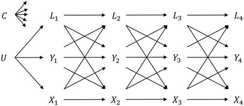
While working with the causal DAG in Figure 1, we make the implicit assumption that it correctly represents the underlying causal structure between SSC, SE, and the time-varying and time-invariant covariates (Imbens, 2019). Arguably, the lag-1 process as encoded in the DAG of Figure 1 is an oversimplification, as empirical processes might include effects that extend beyond a single time interval (i.e., lag-2 and longer; Little, 2013, p. 203). Additionally, lag-0 effects can be added to the DAG to represent contemporaneous effects. Such effects are commonly assumed in longitudinal biomedical research, for example when the decision to give an individual a treatment X at a particular time point depends on a range of previous covariates, as well as current values of covariates such as blood results. Recently, Muthén and Asparouhov (2022a) argued that lag-0 effects may also be realistic in psychological research when data are collected with long time intervals and measurements referring to past experiences (e.g., when X_t refers to a construct in the past thirty days, whereas Y_t refers to a construct “at this moment”). As the omission of such lag-0 or lag-2 (and longer) effects from the causal DAG is a stronger assumption than their inclusion (i.e., it amounts to constraining these paths to zero; Bollen & Pearl, 2013), it is advisable to include these effects whenever there is doubt about their existence, and to adjust for them in statistical analyses. For didactical reasons, we start with the simplified DAG in Figure 1, but in Section 4, we discuss in more detail the addition of lag-0 and lag-2 causal dependencies to the DAG, and how this impacts the cross-lagged panel modeling and SNMM approaches.

2.2. Cross-Lagged Effects and Joint Effects

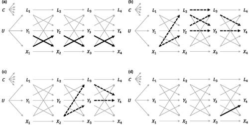
Figure 2(a) visualizes cross-lagged effects in the causal DAG of Figure 1. Characteristically, cross-lagged effects are bidirectional, implying that SSC and SE take on the role of both presumed cause and outcome: At the first wave SSC and SE are presumed causes, at the final wave SSC and SE are outcomes, and at the intermediate waves SSC and SE are both. In psychological research oftentimes each dependency (i.e., arrow) independently is a target of inference. That is, when interested in cross-lagged effects and assuming the causal structure of Figure 1, we target six causal effects: Three cross-lagged effects from SSC to subsequent SE, and three cross-lagged effects from SE to subsequent SSC. Although the focus is typically only on lag-1 relationships, in the epidemiological and biostatistical literature, effects of exposure regimes are more commonly investigated (also sometimes referred to as exposure sequences or exposure history; Wallace et al., 2017).

Figure 2. Representation of the causal dependencies that are targeted by research questions on reciprocal, cross-lagged effects, and joint effects. (a) Reciprocal, cross-lagged effects. (b) Controlled direct effect of X₁ on Y₄. (c) Controlled direct effect of X₂ on Y₄. (d) Controlled direct effect of X₃ on Y₄.

Regimes can be regarded as treatment strategies that span multiple time points. An example is a regime in which individuals are made to experience their highest possible satisfaction with their social contacts at each of the four measurement occasions. Suppose that “highest possible satisfaction” is denoted by a score of 5 on our SSC-scale, this regime could then be represented as $\{x_1=5,x_2=5,x_3=5,x_4=5\}.$ Another example would be a regime in which the individuals are made to be moderately satisfied at the first two occasions (corresponding to a score of 2), and to be completely unsatisfied at the third and fourth occasion (corresponding to a score of 0), $\{x_1=2,x_2=2,x_3=0,x_4=0\}.$ For simplicity of notation, we denote such regimes as $\{5,5,5,5\}$ and $\{2,2,0,0\},$ respectively. Contrasting end-of-study outcomes that follow from two different exposure regimes then allows researchers to assess the average causal effect (ACE) of being exposed to one specific regime compared to another specific regime. Such contrasts are also known as joint effects, where “joint” refers to the exposures at multiple time points combined.

For continuous exposures and the constructs typically of interest in psychological research, it might be difficult to conceive of a policy or intervention with which individuals can be made to experience exactly a particular level of satisfaction with their social contacts. Therefore, it might be more interesting to look at the joint effect of increasing an individual’s satisfaction by one unit compared to the level of satisfaction that individuals would naturally take on. This joint effect can represented as a contrast of end-of-study outcomes following the $\{x_1,x_2,x_3,x_4\}$ regime versus the $\{x_1+1,x_2+1,x_3+1,x_4+1\}$ regime, where the former represents the natural satisfaction of individuals, and the latter the natural satisfaction of individuals increased by one unit.

Such joint effects can be decomposed into multiple controlled direct effects (CDEs), specifically (1) the effect of X₁ on end-of-study Y₄, which does not through later versions of X; (2) the effect of X₂ on end-of-study Y₄ which does not go through later versions of X; and (3) the effect of X₃ on end-of-study Y₄ which does not go through later X (Figures 2(b–d), respectively; Daniel et al., 2013). This decomposition is useful later for understanding how SNMMs are build up. For researchers familiar with mediation analysis in SEM, the term “controlled direct effect” might be confusing terminology in this context as the intermediate process would be regarded as a set of indirect effects, rather than direct. For SNMMs, however, the term “controlled” in CDE refers to the fact that values of later SSC are held constant at a particular value (or set of values), whereas the term “direct” refers to the fact that the underlying intermediate process by which SSC at a particular time point affects end-of-study SE is not modeled, but that rather a single estimate summarizing this intermediate process is obtained (Tompsett et al., 2022; Wallace et al., 2017). To accentuate the fact that for CDEs in the context of SNMMs the intermediate process is not our target of inference, the intermediate dependencies for the CDEs of X₁ and X₂ in Figures 2(b,c) appear as dotted arrows.

Let us zoom in on the CDE of X₁ on the end-of-study outcome Y₄ in Figure 2(b). This can alternatively be represented as the difference between the outcome following the regime $\{x_1+1,x_2,x_3\}$ and the outcome following the regime $\{x_1,x_2,x_3\}$—i.e., the effect of a one-point increase in SSC at the first measurement occasion on end-of-study SE, while keeping future levels of SSC constant at values x₂ and x₃ for everyone. These values can be anything, but for interpretational reasons, researchers might set x₂ and x₃ to the mean SSC score, or, as commonly done when exposure is binary, to zero. Even more generally, the CDE can be represented as a contrast of outcomes following the regimes $\{x_1^{*},x_2,x_3\}$ versus $\{x_1,x_2,x_3\}$ to represent the effect of an arbitrary increase of SSC at the first measurement occasion. We ignore X₄ here as, based on the causal DAG in Figure 1, it has no causal effect on the end-of-study outcome. Similarly, the CDE of X₂ can be regarded as a contrast of outcomes following the regimes $\{x_1,x_2^{*},x_3\}$ versus $\{x_1,x_2,x_3\}.$ In this contrast, we control for exposure before time point 2 ($X_1=x_1$), and future exposure ($X_3=x_3$). Finally, the CDE of X₃ can be represented as a contrast of $\{x_1,x_2,x_3^{*}\}$ and $\{x_1,x_2,x_3\}.$ Finally, for this particular DAG, the CDE of X₃ and the cross-lagged effect of X₃ concern the same dependency in the causal DAG, $X_3\to Y_4.$ However, note that this (causal) equivalence does not hold generally (e.g., when lag-0 effects of the time-varying covariate to the outcome are added to the causal DAG).

2.3. Conceptual Differences Between Cross-Lagged Effects and Joint Effects

There are multiple conceptual differences between cross-lagged effects that tend to be the focus in psychological research, and joint effects that are more typically focused on biomedical research. These differences not only affect the interpretation of the effects, but also have statistical ramifications. First, research questions about cross-lagged effects in a psychological context are typically bidirectional in nature: Researchers investigate if effects between variables go from X to Y, from Y to X, and if both processes are at work, which process is “causally dominant” (Rogosa, 1980). Instead, investigations of joint effects in the literature are predominately unidirectional, with researchers deciding a priori which specific causal process (i.e., which “causal direction”) is studied. Nonetheless, joint effects can also be studied in both directions (e.g., Li et al., 2016), but this would be done as a seperate analysis.

Second, the role variables take on in a causal process depends on the causal effect that is targeted. For cross-lagged effects, six variables are exposures, namely X₁, Y₁, X₂, Y₂, X₃, and Y₃, and six variables are outcomes, namely X₂, Y₂, X₃, Y₃, X₄, and Y₄. Instead, for joint effects, the exposure is a single variable measured at multiple time points, X_t. Moreover, the majority of the studies investigating joint effects concern a single outcome, usually measured at the end of a study (e.g., Y₄). However, when an outcome is measured repeatedly (as done in a cross-lagged panel design), SNMMs can be extended to include time-varying outcomes as well (Vansteelandt & Sjolander, 2016).

The role of time-varying covariates also changes. For example, the cross-lagged effect $X_3\to Y_4$ is confounded by L₂ via the paths $X_3\leftarrow L_2\to L_3\to Y_4$ and $X_3\leftarrow L_2\to Y_3\to Y_4.$ This implies that the time-varying covariates at time point 2 should be controlled for in a statistical analysis. In contrast, for the joint effect of X, L₂ is both a confounder and a mediator: It is a confounder for the CDE of X₃ (i.e., it is a common cause on the paths $X_3\leftarrow L_2\to Y_3\to Y_4$ and $X_3\leftarrow L_2\to L_3\to Y_4$), but a mediator for the CDE of X₁ (it lies on the paths $X_1\to L_2\to L_3\to Y_4$ and $X_1\to L_2\to Y_3\to Y_4$). Such a “double role” complicates statistical analyses, as attempts to estimate the joint effect with standard regression methods—for example, a linear regression of Y₄ on all exposures X₁, X₂, X₃, and all confounders simultaneously—is incorrect: Controlling for L₂ leads to overcontrol bias for the CDE of X₁, whereas not controlling for L₂ leads to confounder bias in the CDE of X₃ (VanderWeele et al., 2016). In the causal inference literature, this problem is referred to as exposure-confounder feedback, and the causal inference approaches by Robins have been developed specifically to tackle this problem (Robins & Greenland, 2000). In Section 3, we discuss how exposure-confounder feedback is dealt with in both cross-lagged panel models, and SNMMs with G-estimation.

Third, cross-lagged effects and joint effects relate to different time lags at which the causal process operates. In general, estimates of causal effects depend critically on the size of the time interval between subsequent measures (Gollob & Reichardt, 1987; Kuiper & Ryan, 2018; Voelkle et al., 2012). Therefore, estimates of cross-lagged effects are interpreted as causal effects that take one time-lag to materialize. For our empirical example, we use data from the Longitudinal Internet studies for the Social Sciences (LISS) in which measurements were taken on a yearly basis (more information about the LISS panel can be found at https://www.lissdata.nl; Scherpenzeel, 2018). Hence, an estimate of the cross-lagged effect of SSC on SE is the expected change in SE one year later for a one-unit increase in SSC. In contrast, the joint effect is a combination of causal effects at varying time-lags: The CDE of X₁ relates to three years, the CDE of X₂ relates to two years, and the CDE of X₃ relates to one year. It can thus be regarded as a mix of shorter- and longer-term effects, describing the effect of repeated yearly interventions on SSC across a three-year period.

2.4. Causal identification assumptions

When estimating the effects discussed above from empirical data, a causal interpretation thereof relies critically on both causal identification assumptions and parametric assumptions. While the focus of this article is on a comparison of the parametric assumptions that a CLPM in SEM and an SNMM with G-estimation make, causal identification assumptions are fundamental to a causal interpretation of estimates. Introductions to causal identification assumptions are given by Morgan and Winship (2014); Imbens and Rubin (2015). Therefore, we briefly discuss two central causal identification assumptions here, namely conditional exchangeability and consistency. The plausibility of these assumptions for our empirical example is elaborated upon in the Discussion section; for the purpose of this article, we continue as if these assumptions hold.

Both consistency and exchangeability concern potential outcomes and observed variables. A potential outcome, denoted by Y^x, is an outcome for a particular individual at a particular point in time that would be observed if the individual had exposure X = x (Rubin, 1974; Splawa-Neyman et al., 1990). For example, suppose that we are looking at SSC only at time point 3; then Y⁵ would be the end-of-study SE if an individual had an SSC score of five at time point 3 (i.e., $x_3=5),$ and Y¹ would be the end-of-study SE if an individual had an SSC score of one (i.e., $x_3=1).$ In reality, an individual has only a single SSC score at time point 3, and thus we can only observe one potential outcome (the factual) while the others remain unknown (the counterfactuals). In similar vein, we can have potential outcomes for exposure regimes, $Y^{\{x_1,x_2,x_3\}},$ which is the outcome for a particular individual that would be observed if the individual had the exposure regime $\{x_1,x_2,x_3\}.$ Potential outcomes are the fundamental building blocks of much of the causal inference literature as they are used to define in great detail which particular (hypothesized) causal effects are of interest for a study. In fact, we have already implicitly used these above to explain joint effects as differences between end-of-study outcomes that follow from two different regimes (i.e., as a contrast of two potential outcomes). What causal identification assumptions do, is link the causal effect of interest (in terms of a contrast between two specifically defined potential outcomes), to the data from which we attempt to estimate this effect.

The consistency assumption states that the potential outcomes can be tied to observed variables, meaning that, for example, the potential outcome $Y^{\{5,5,5\}}$ is the same as the observed Y for individuals with exposure regime {5, 5, 5} (Hernán & Robins, 2020). In practice, this assumption implies that these constructs are well-defined, including being specific about the (hypothetical) intervention that could set an individual’s exposure regime to {5, 5, 5} (even if the intervention is impractical, unethical, or impossible to carry out; Robins & Greenland, 2000). For our example, we might consider changing an individual’s SSC by having participants partake in therapy, or perhaps we can imagine implementing a public a policy in which every individual gets an amount of money each month that they can spend on social events with others. The consistency assumption also highlights a fundamental challenge in psychological research, which is conceiving of practical interventions that change only the exposure of interest (Eronen, 2020). If multiple versions of an intervention on SSC have different effects, then observed outcomes might not necessarily equal the potential outcomes, and it remains unclear how numerical estimates of “the effect” relate to the “the effect” as formulated in the research question (i.e., we than have an “ill-defined” causal effect; Hernán, 2016; Pearl, 2018).

The assumption of (conditional) exchangeability states that the potential outcomes are independent from their observed value on the exposure X (conditional on a set of covariates).² It is a condition that is reasonable in the context of a randomized controlled trial, but is likely to be violated to some degree in nonexperimental settings. To make the assumption plausible, researchers condition on covariates that confound the targeted effect. The set of covariates to be adjusted for can be determined using the d-separation rules by Pearl (1995).³ In practice, the major challenge is making sure that we have measured enough covariates to adjust for the biasing effect of confounders. Unfortunately, this cannot be tested with data, but should be evaluated by the researcher based on theory, existing literature, and/or expert opinion (Goetghebeur et al., 2020; Petersen & Van der Laan, 2014). Note that the assumption of exchangeability merely concerns which confounders should be accounted for, not how they should be accounted for. The latter concerns the act of estimation rather than identification, and which is where SEMs and SNMMs with G-estimation are inherently different.

2.5. Conclusion

Traditionally, psychological research has typically focused on cross-lagged effects, whereas biomedical research was more commonly concerned with joint effects. However, there is no inherent reason why joint effects would not be interesting for psychology. For our empirical example, a research question concerning a joint effect could be: “For Dutch young adults who have moved out of their parents’ house in the past year, what is the joint effect of increasing their satisfaction with one’s social contacts for three years on self-esteem three years after moving out, compared to the satisfaction with one’s social contacts that they would naturally have during these three years?” Again, a big challenge here is making this research question well-defined by conceiving of an intervention by which we can change an individuals’ satisfaction with social contacts. For the purpose of this study, we continue as if the consistency assumption holds, and discuss how our research question can be investigated using several estimation approaches.

3. Estimation approaches

We focus on two estimation approaches: The use of cross-lagged panel models (CLPMs) within the framework of structural equation modeling, and the use of a SNMM with G-estimation. We specifically discuss the parametric assumptions underlying CLPMs and SNMMs: Which dependencies of a causal DAG do researchers need to correctly specify the functional form of, and how are differences herein across approaches (dis)advantageous when the goal is to estimate the targeted causal effect? To help clarify some key characteristics of SNMMs with G-estimation, we also briefly discuss a repeated multiple regression approach for estimating joint effects.

3.1. CLPMs in the Structural Equation Modeling Framework

One of the most popular classes of structural equation models in psychology for assessing prospective causal relations between variables is CLPMs (Usami et al., 2019; Zyphur et al., 2020a; 2020b). In this section, we outline some of the defining characteristics of this specific structural equation modeling approach, and subsequently discuss its advantages and disadvantages.

3.1.1. The Basic Idea

CLPMs typically attempt to model the entire causal structure of the process under study using linear relations. In a longitudinal context, this includes specifying how (1) the outcome depends on previous exposure and covariates; (2) the time-varying exposure depends on previous exposures and covariates; and (3) the covariates depend on previous exposures and covariates. For our example, this modeling approach implies that the causal DAG in Figure 1 would be interpreted as a path diagram, with all individual dependencies (arrows) specified. In practice, covariances between the residuals at the same wave are usually added to the model to capture the direct effects of unobserved time-varying confounders whose effects are limited to a single time point, and who themselves show no dependencies over time. Such confounding variables are not assumed in the causal DAG of Figure 1, which implies that estimation of residual covariances would be redundant.

In practice the dependencies in CLPMs in SEM are typically assumed to be linear; nonlinear relationships are rarely considered (although, in principle, it is possible to specify them, for example Harring & Zou, 2023; Mulder et al., 2024). If the assumed causal structure in the causal DAG is correct, and all parametric assumptions underlying the CLPM are true (i.e., all effects are linear, residuals are normally distributed), then the CLPM results in unbiased estimates of each path, and estimates of cross-lagged effects can be read off directly as regression coefficients of the boldfaced paths in Figure 2(a). The CDEs can then be obtained as relatively simple linear combinations of parameter estimates on the causal paths of interest. For example, using the path tracing rules by Wright (1934), the CDE of X₁ is a combination of the regression coefficients on the paths $X_1\to L_2\to L_3\to Y_4;$ $X_1\to L_2\to Y_3\to Y_4;$ $X_1\to Y_2\to L_3\to Y_4;$ and $X_1\to Y_2\to Y_3\to Y_4.$ This CDE is thus the effect of X₁ on Y₄ that is mediated by all covariates in L and previous Y, and does not go through future X’s. The same principle applies for the specification of the CDEs of X₂ and X₃.

3.1.2. Advantages

One advantage of this estimation approach is that the problem of exposure-confounder feedback is not applicable: By modeling the entire (assumed) data generating mechanism, the researcher has control over which paths to combine to get estimates of the effect of interest. Furthermore, reliance on (many) parametric assumptions results in efficient use of the data, leading to relatively small standard errors. Secondary advantages are derived from the structural equation modeling framework that CLPMs are specified in. For example, a major advantage is that SEMs can include latent variables, which can be used to study latent constructs using multiple indicators, to account for measurement error and unobserved heterogeneity in the constructs, among other things (Kenny & Zautra, 1995; Mulder & Hamaker, 2021; Usami, 2021). Furthermore, many structural equation modeling software packages can handle various missing data patterns through the use of full information maximum likelihood (FIML; Arbuckle, 1996). This is convenient, as missing data are the norm rather than the exception in nonexperimental longitudinal settings (Van Buuren, 2018, p. 7).

3.1.3. Disadvantages

From a causal inference point-of-view there is the concern that by parameterizing the entire causal process as a linear process, there is increased risk of model misspecification and consequently bias: Parametric misspecication of any dependency in the CLPM—such as wrongly assuming a causal effect to be linear, whereas, in fact, it is nonlinear—can lead to bias that propagates to other parts of the model as well (cf. Mulder et al., 2024; VanderWeele, 2012). In fact, with the CLPM approach outlined above, parts of the causal DAG are modeled that are not necessary for identification and estimation of targeted causal effects. Take the effect $X_3\to Y_4$ for example, which is of interest as both a cross-lagged effect, and as the CDE of X₃. Obtaining an unbiased estimate requires, amongst other things, correctly adjusting for covariates that could confound this relationship (i.e., the conditional exchangeability assumption). Based on the causal DAG in Figure 1 and using the d-separation rules, it can be shown that adjustment for covariates L₃, Y₃, and C is enough to block all noncausal pathways between X₃ and Y₄: It does not require modeling how these covariates themselves depend on previous covariates. However, since CLPMs are concerned with modeling a data generating mechanism in its entirety, the causal structure of these covariates is typically modeled as well. This is often required to achieve desirable levels of model fit for the model as a whole; yet, it is redundant if the researcher is exclusively interested in obtaining unbiased estimates of specific causal dependencies. Similar arguments apply when estimating other cross-lagged effects or CDEs. Van der Laan and Rose (2011) point out that such unnecessary modeling increases the potential for model misspecification, and ultimately results in bias for the estimates of the targeted causal effects (see also Naimi et al., 2016). This point has been made before in the context of CLPMs (Allison et al., 2017; Bollen, 1989), but does not appear to have been picked up in current structural equation modeling practices.

A second disadvantage of CLPM approaches in SEM is that the incorporation of multiple time-varying covariates can quickly become unwieldy. This also applies if bidirectional lag-0, or lag-2 effects (or further) are to be included, or if quadratic terms are added to the model to specify nonlinear dependencies (Muthén & Asparouhov, 2022a). Such extensions (and many others) can dramatically increase the number of parameters that need to be estimated, and can steeply increase the size of the covariance matrix that needs to be modeled, thereby requiring increasingly large sample sizes to find a stable solution for the parameter estimates. For our example, if we were to interpret the causal DAG in Figure 1 as a path diagram, it would include (at least, excluding covariances, and residual covariances) 65 parameters, that is: 39 regression parameters, 1 variance, and 12 residual variances, 1 mean, and 12 intercepts. The inclusion of 1 additional time-varying covariate with a similar lag-1 causal structure adds 21 regression coefficients, 4 residual variances, and 4 intercepts to the model. As psychological mechanisms can involve a plethora of time-varying covariates that researchers (should) want to adjust for, attempts to model the entire causal system can quickly become practically prohibitive.

Third, including categorical variables as covariates in CLPMs is challenging, as the estimated regression coefficients are then on different scales, making it difficult to combine coefficients to compute CDEs. Suppose that a time-varying covariate in L is categorical, for example drug use. This implies that regressions of drug use on other variables concern logistic or probit regressions, resulting in logistic (e.g., odds ratios) or probit regression coefficients, respectively (Muthén et al., 2016). These then need to be combined with linear regression coefficients from other paths in the SEM, for instance $L_3\to Y_4,$ to compute the CDEs of interest, which requires specific computational methods. Such computations are possible for relatively simple situations with a single categorical time-varying covariate, but this process becomes increasingly involved when the number of time-varying categorical covariates increases (for more details, see Muthén et al., 2016; Nguyen et al., 2016).

3.2. Repeated multiple regression

In the causal inference literature, estimation approaches are usually presented in the context of exposure-confounder feedback (VanderWeele, 2021). In the presence of this problem, standard regression methods that attempt to simultaneously estimate all CDEs that make up a particular joint treatment effect—for example, by regressing the outcome on all exposures and covariates—are inadequate, leading to biased estimates of joint effects. However, it is possible to use standard regression methods in a “repeated” manner: Multiple standard regression models are then fitted, one for the estimation of each CDE separately. This makes it possible to work with distinct sets of covariates to adjust for confounding, thereby preventing the problem of exposure-confounder feedback. Although this exact method is not commonly used in practice, we explore it here as a first step towards the explanation of SNMMs with G-estimation.

Figure 3 illustrates the three regression models that must be specified to estimate the joint effect of X on end-of-study Y₄ (assuming the causal DAG in Figure 1). We can determine which sets of covariates to condition on from the causal DAG in Figure 1 and using the d-separation rules by Pearl (1995). For this example, the smallest adjustment set for closing all back-door paths from X₃ to Y₄, is the set of variables L₃, Y₃, and C, as shown in Figure 3(a). Under the causal identification assumptions (Section 2.4) and the parametric assumptions of this regression model (i.e., the functional form of the relationship between the covariates in L₃ and the outcome is correct, and there is no interaction between exposure and previous exposures and confounders), the regression coefficient of X₃ obtained with this regression model is an unbiased estimate of the CDE of X₃ on Y₄. Alternatively, the regression model can be used akin to the “regression estimation” method described by Schafer and Kang (2008), which includes making predictions of individuals’ potential outcomes under two values of X₃ (and using observed values on all the covariates), and then compute the CDE of the exposure X₃ as the difference between the average outcomes under both X₃-values.

Figure 3. Overview of the regression models that need to be correctly specified for estimating the joint effect of X on Y using standard regression methods. (a) Regression model for estimating CDE of X₃ on Y₄. (b) Regression model for estimating CDE of X₂ on Y₄. (c) Regression model for estimating CDE of X₁ on Y₄.

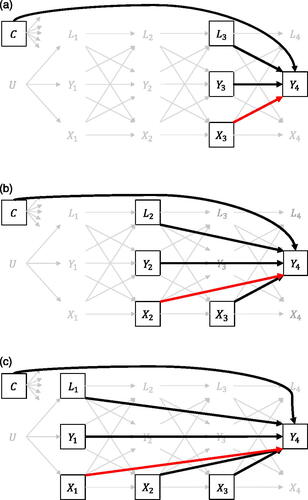
To estimate the CDE of X₂, we need to fit a second regression model, where this time we adjust for the set L₂, Y₂, C, and X₃ to control for confounding, and as shown in Figure 3(b). Adjustment for X₃ is required to block the effect of X₂ on Y₄ that goes through the future exposure (by definition of a joint effect, this is not allowed). In this regression model, we can block the effect of X₂ on Y₄ that goes through X₃ simply by including X₃ as an additional covariate in the model. Similar to the CDE of X₃ we can interpret the regression coefficient of X₂ is an unbiased estimate of the CDE of X₂ (given the causal identification assumptions, and the parametric assumptions of the specified regression model), or use this model for regression estimation to obtain an estimate of the causal effect.

Finally, the procedure for estimation of CDE of X₁ is similar, but now using the regression model illustrated in Figure 3(c). Here we include L₁, Y₁, and C as covariates to control for confounding by C and U. Future exposures X₂ and X₃ are included in the regression model to block the effect of X₁ on Y₄ through X₂ and X₃.

Compared to a CLPM, the regression models in this repeated procedure rely on the specification of much fewer dependencies to get unbiased estimates of the CDEs. Specifically, no model is specified for time-varying covariates L and Y (before the end-of-study), and the CDEs are specified directly rather than indirectly through the individual dependencies underlying them. For this reason, this approach has a lower risk of parametric model misspecification. Furthermore, these regression models can also be fitted within the SEM framework. As such, researchers can combine advantages of SEM techniques (e.g., the inclusion of latent variables, the use of FIML for missing data handling), with the advantages of this sequential regression approach.

3.3. Linear SNMMs Using G-Estimation

SNMMs with G-estimation are described as a flexible and robust method for investigating joint effects in the presence of exposure-confounder feedback (Vansteelandt & Joffe, 2014). It shows resemblance with the repeated multiple regression approach discussed above, in that the CDEs are estimated separately as well, and that G-estimation of the CDEs of X₂ and X₁ requires adjustment for future exposures. However, the use of SNMMs with G-estimation adjusts for future exposures differently; additionally requires modeling the exposure; and can be doubly-robust, implying that estimates of causal effects are consistent, and thus converge to the true value as sample size increases, even if part of the model is misspecified.⁴ This latter characteristic is generally considered appealing from a causal inference point-of-view (cf., Kang & Schafer, 2007; Schafer & Kang, 2008). However, what makes this approach challenging for psychological researchers to learn about is that (1) its use in the literature is described for heterogeneous research problems, for instance for assessing joint effects, mediation, or survival rates; (2) there exist multiple different G-estimation methods for fitting SNMMs to data; (3) these different methods each have different features that make them (dis)advantageous for specific research settings; and (4) there is little comprehensive software that has implemented all these methods. Therefore, our goal in this subsection is to provide the reader with a basic understanding of what an SNMM is, what the essence of G-estimation is, and what the (dis)advantages of this approach are compared to CLPMs. We focus specifically on the G-estimation method for linear SNMMs as described by Vansteelandt and Sjolander (2016) and Loh and Ren (2023a), with data in wide-format.

3.3.1. The Basic Idea

Joint effects are a collection of CDEs (Daniel et al., 2013), and CDEs can be represented as contrasts of end-of-study outcomes that follow from two different regimes (Section 2.2). An SNMM is a model for these contrasts, where each CDE is equated to a causal parameter ψ_t. G-estimation is a sequential process that estimates the ψ_t’s, starting with the last CDE, and then working backwards through time.

The joint effect can be represented as a comparison of the regimes $\{x_1,x_2,x_3\}$ with $\{x_1+1,x_2+1,x_3+1\}.$ We start with the CDE of X₃ on Y₄, which can be parameterized as (1) $$\mathbb{E}(Y_4^{\{x_1,x_2,x_3+1\}}-Y_4^{\{x_1,x_2,x_3\}}|C=c,X_2=x_2,L_2=l_2,Y_2=y_2)={\psi }_3.$$(1)

The term on the left-hand side is the difference in the expected outcome of end-of-study Y₄ if all individuals followed the regime $\{x_1,x_2,x_3+1\}$ versus if all followed the regime $\{x_1,x_2,x_3\};$ hence, the only difference is in the exposure at the third time point. We condition on covariates that are sufficient to block all noncausal paths between X₃ and Y₄ based on the causal DAG in Figure 1. Rather than conditioning on the smallest adjustment set used in the repeated regression method discussed above, we decided to condition on the covariates C, X₂, L₂, and Y₂. The reason for this is that in fitting the model (as discussed later in this Section), we need to predict the exposure X₃, and based on the causal DAG in Figure 1, it makes more sense to do this with variables prior to X₃ rather than variables measured contemporaneously with X₃. The causal effect is equated to the parameter ψ₃. For the purpose of this paper, we start with a basic linear SNMM here (i.e., there are no interaction terms implying an absence of moderation, and no quadratic terms), although Equation (1)(1) $$\mathbb{E}(Y_4^{\{x_1,x_2,x_3+1\}}-Y_4^{\{x_1,x_2,x_3\}}|C=c,X_2=x_2,L_2=l_2,Y_2=y_2)={\psi }_3.$$(1) can be extended with interactions between exposure and (time-varying) covariates.

To estimate ψ₃, we make use of G-estimation, which is any estimation procedure that can be derived from the conditional exchangeability assumption (Vansteelandt & Joffe, 2014). As discussed in Subsection 2.4, conditional exchangeability states that the potential outcomes are independent from observed exposure conditional on covariates. Assuming only linear relationships, this independence assumption can be written as (2) $$\mathit{\text{Cov}}(Y_4^{\{x_1,x_2,x_3^{*}\}},X_3|C,X_2,L_2,Y_2)=0,$$(2) where $Y^{\{x_1,x_2,x_3^{*}\}}$ represents the potential outcome for the treatment regimes with x₁ and x₂ set to their actual observed values, while $x_3^{*}$ is set to a specific value, for instance zero, for all people.

Equation (2)(2) $$\mathit{\text{Cov}}(Y_4^{\{x_1,x_2,x_3^{*}\}},X_3|C,X_2,L_2,Y_2)=0,$$(2) may at first appear unrelated to our parameter of interest ψ₃, and also rather impractical, as the potential outcome term $Y^{\{x_1,x_2,x_3^{*}\}}$ is not actually observed (Naimi et al., 2016). However, through the SNMM, we can connect ψ₃ and Equation (2)(2) $$\mathit{\text{Cov}}(Y_4^{\{x_1,x_2,x_3^{*}\}},X_3|C,X_2,L_2,Y_2)=0,$$(2) (Vansteelandt & Joffe, 2014). To see this, suppose we want to compute the expected end-of-study SE score for each individual if their SSC score at the third wave had been set zero, that is, $Y^{\{x_1,x_2,0\}};$ however, we have observed $Y^{\{x_1,x_2,x_3\}}.$ Recall that ψ₃ is the difference in the (expected) potential outcomes, when there is a one unit difference in x₃ (when going from the observed x₃ to $x_3+1$). Hence, when going from the actual observed x₃ to $x_3^{*}=0,$ the (expected) change in the potential outcomes is $Y_4^{\{x_1,x_2,x_3\}}-Y_4^{\{x_1,x_2,0\}}={\psi }_3{x}_3.$ Since, under consistency, $Y_4^{\{x_1,x_2,x_3\}}=Y_4$ (i.e., our observed end-of-study outcome), this implies we can write (3) $$Y_4^{\{x_1,x_2,0\}}=Y_4-{\psi }_3{X}_3.$$(3)

Plugging Equation (3)(3) $$Y_4^{\{x_1,x_2,0\}}=Y_4-{\psi }_3{X}_3.$$(3) into Equation (2)(2) $$\mathit{\text{Cov}}(Y_4^{\{x_1,x_2,x_3^{*}\}},X_3|C,X_2,L_2,Y_2)=0,$$(2) then leads to (4) $$\mathit{\text{Cov}}(Y_4-{\psi }_3{X}_3,X_3|C,X_2,L_2,Y_2)=0.$$(4)

This shows the essence of G-estimation: Finding a value for ψ₃ such that Equation (4)(4) $$\mathit{\text{Cov}}(Y_4-{\psi }_3{X}_3,X_3|C,X_2,L_2,Y_2)=0.$$(4) holds.⁵

3.3.2. G-estimation for Linear SNMMs by Vansteelandt and Sjolander

Multiple G-estimation methods have been developed for estimating ψ₃. For example, Hernán and Robins (2020) describe a grid search, simply plugging in a range of values for ψ₃ until you find the value such that Equation (2)(2) $$\mathit{\text{Cov}}(Y_4^{\{x_1,x_2,x_3^{*}\}},X_3|C,X_2,L_2,Y_2)=0,$$(2) holds. Vansteelandt and Sjolander (2016), however, describe a procedure (i.e., a closed-form estimator) for linear SNMMs that relies on fitting regression models for both the exposures and the outcome; a model for the covariates is not required. How this procedure can be derived from the conditional exchangeability assumption is shown in their appendix.

This method consists of three steps. First, a regression model for the exposure X₃ is specified, conditional on a set of covariates for blocking all noncausal paths, X₂, L₂, Y₂, and C. Figure 4(a) illustrates this exposure model, which Vansteelandt and Sjolander (2016) also refer to generally as the propensity score (PS) model. Second, from the exposure model, predicted values for the exposure X₃ are calculated, which we denote by ${\widehat{X}}_3.$ These values would be referred to as “propensity scores” if the exposure was dichotomous, but work essentially the same for continuous exposures. The idea of this score is that it contains all information from variables that are needed to block noncausal paths that contribute to the association between the exposure and the outcome (Imbens & Rubin, 2015). Third, a regression model for the outcome is specified conditional on the observed exposure X₃, the predicted exposure ${\widehat{X}}_3,$ and the covariates X₂, L₂, Y₂, and C, thereby blocking noncausal pathways. If only the exposure model in step 1 is correctly specified, then this procedure is comparable to regression adjustment on the propensity score, and the additional covariates only increase precision (Vansteelandt & Daniel, 2014). If only the covariate-outcome relations in the outcome model are correctly specified, then we block all noncausal paths akin to the repeated multiple regression approach, and the additional PS covariate merely leads to an overfitted outcome model. The regression coefficient of X₃ in the outcome model is the G-estimate of ψ₃, that is ${\widehat{\psi }}_3:$ It is unbiased with both the exposure model and the outcome model correctly specified, and consistent when only one of both models is correct (i.e., this method is doubly-robust).

Figure 4. Overview of the regression models that need to be correctly specified in the fitting procedure of a linear SNMM. A square around a variable implies that this variable needs to be included as a variable in the model. (a) Exposure model for X₃. (b) Outcome model for estimation of the CDE of X₃. (c) Exposure model for X₂. (d) Outcome model for the CDE of X₂ on end-of-study the X₃-free end-of-study outcome. (e) Exposure model for G-estimation of Equation 7(7) $$\mathbb{E}(Y_4^{\{x_1+1,0,0\}}-Y_4^{\{x_1,0,0\}}|C=c,U=u)={\psi }_1.$$(7) . Future exposure is set to X₃ = 0. (f) Outcome model for the CDE of X₁ on the X₂-and-X₃-free end-of-study outcome. Future exposures are set to X₂ = 0 and X₃ = 0.

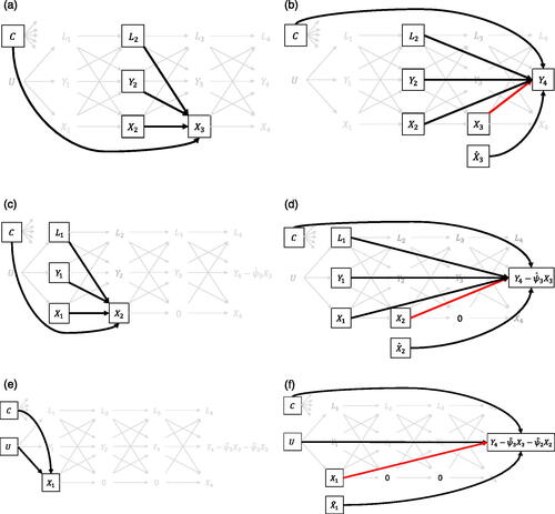
This entire procedure works similarly for estimating the CDEs of X₂ and X₁. In the SNMM, the CDE of X₂ is parameterized as (5) $$\mathbb{E}(Y_4^{\{x_1,x_2+1,0\}}-Y_4^{\{x_1,x_2,0\}}|C=c,L_1=l_1,Y_1=y_1)={\psi }_2,$$(5)

The term on the left-hand side represents the difference in the expected outcome of end-of-study Y if all individuals were exposed to the regime $\{x_1,x_2+1,0\}$ versus if all individuals were exposed to $\{x_1,x_2,0\}.$ Again, we condition on covariates to block all noncausal paths, C, X₁, L₁, and Y₁. To get the unique effect of X₂ (i.e., not going through future exposure), we additionally need to adjust for future exposure. Unlike the repeated multiple regression approach—in which we included future exposure as an additional covariate in the model—this method relies on computing a new outcome variable as if everyone had the same value on future exposures. The reasoning behind this is that when future exposures are a constant, they cannot have a causal effect on the outcome. In practice, future exposure value is commonly set to zero for all individuals such that the new outcome can be computed by (6) $$Y_{\text{4, blipped‐down}}=Y_4-{\widehat{\psi }}_3{X}_3.$$(6)

This equation is similar to Equation (3)(3) $$Y_4^{\{x_1,x_2,0\}}=Y_4-{\psi }_3{X}_3.$$(3) , except that we now plug ${\widehat{\psi }}_3$ into ψ₃. The new outcome is also referred to as the “blipped-down version of Y₄” or the “candidate counterfactual”, and represents the outcome if unaffected by the exposure at occasion 3. To estimate ψ₂, we first estimate an exposure model again; regressing X₂ on the covariates X₁, L₁, Y₁, and C (Figure 4c). Second, we compute the predicted values of exposure at time point 2, the PS score ${\widehat{X}}_2$ for every person. Third, we fit a regression model for the blipped-down outcome $Y_{\text{4, blipped‐down}}$ conditional on the covariates, observed exposure X₂, and predicted exposure ${\widehat{X}}_2$ (Figure 4(d), note X₃ is set to 0). The regression coefficient of X₂ in the outcome model is then an estimate of ψ₂.

Finally, in the SNMM, the CDE of $X_1$ is parameterized as (7) $$\mathbb{E}(Y_4^{\{x_1+1,0,0\}}-Y_4^{\{x_1,0,0\}}|C=c,U=u)={\psi }_1.$$(7)

The term on the left-hand side represents the difference in the expected outcome of end-of-study $Y_4$ if all individuals were exposed to the regime $\{x_1+1,0,0\}$ versus if all individuals were exposed to $\{x_1,0,0\}$. To block all noncausal pathways between $X_1$ and the outcome, we need to control for the variables in C and U. However, the issue is that in cross-lagged panel research, U is often unobserved, because measurements tend to commence in an ongoing process, and hence realizations of X, Y, and L before the start of measurements (i.e., before $t=1$) are not measured. Nevertheless, these are confounders we want to adjust for. In the epidemiological and biostatistical literature, the first measurements of time-varying covariates are commonly regarded as covariates at baseline (i.e., at $t=0$) that are merely adjusted for, but which are not exposures of interest: That is, we do not attempt to estimate the CDE of $X_0$ on $Y_4$, but only estimate CDEs of exposures after baseline. This is also the strategy that we employ for our explanation here, as well as in the empirical example in Section 4.⁶ In addition to controlling for C and U, we need to control for future exposures by setting them to $X_2=0$ and $X_3=0$. As such, a new blipped-down version of $Y_4$ is computed for every person by (8) $$Y_{\text{4, blipped‐down}}=Y_4-{\widehat{\psi }}_3{X}_3-{\widehat{\psi }}_2{X}_2.$$(8)

To estimate ${\psi }_1$, we follow the same procedure: Fitting an PS model for $X_1$ given C, and U (see Figure 4e), computing the predicted exposure ${\widehat{X}}_1,$ and fitting a regression model for the blipped-down outcome given the covariates in C and U, observed exposure $X_1$, and predicted exposure ${\widehat{X}}_1,$ (see Figure 4f). The regression coefficient of $X_1$ in the outcome model is then an estimate of ${\psi }_1$. This completes the procedure for obtaining point estimates for the CDEs of SSC on end-of-study SE using a basic SNMM via G-estimation. To obtain confidence intervals for these estimates, Vansteelandt and Sjolander (2016) recommend the use of non-parametric bootstrapping.

3.3.3. Advantages

Like the repeated multiple regression approach, these linear SNMMs with G-estimation have a lower risk of model misspecification compared to cross-lagged panel modeling approaches in SEM as no model needs to be specified for time-varying covariates L and Y (before the end-of-study), and the CDEs are obtained directly (Naimi et al., 2016). Furthermore, because this procedure is doubly-robust, the reliance on parametric assumptions being correctly specified is further reduced (although Kang & Schafer, 2007, nuance the perceived benefits of doubly-robust methods, showing that when both the exposure and the outcome model are misspecified, doubly-robust methods may actually show worse performance compared to non-doubly-robust counterparts). Additionally, forgoing the need to model the covariates L means that researchers can more easily adjust for multiple time-varying covariates, and it provides them with increased flexibility for specifying functional forms of dependencies in the exposure model and regression model (compared to SEM models).

The basic linear SNMM that we introduced here can be extended such that researchers can explore a wider range of research questions and using a greater variety of data. For example, Vansteelandt and Sjolander (2016) and Tompsett et al. (2022) discuss the inclusion of interactions to investigate effect modification, as well as analyses with time-varying outcomes using generalized estimating equations with data in long-format, allowing for this methodology to be applied to intensive longitudinal data as well. Finally, Loh and Ren (2023b) illustrate how the SNMM fitting procedure can be performed within the SEM framework. As such, researchers can combine advantages of SEM framework (e.g., working with latent variables, potential to use FIML) with the advantages of SNMMs with G-estimation.

3.3.4. Disadvantages

A disadvantage of the SNMM approach is that the implementation of G-estimation of SNMMs in software, for example in R packages such as gestTools (Tompsett et al., 2022) and DTRreg (Wallace et al., 2017), is currently still inflexible. Specifically, these packages are often tailored to situations which include lag-0 effects, and it can be challenging to adjust the data file, and the input for required arguments in such a way that these R packages work for situations without contemporaneous effects (as for our empirical example).

3.4. Conclusion

When comparing CLPMs in SEM with SNMMs with G-estimation, we can summarize their main differences in the following five points. First, compared to CLPMs, SNMMs approaches do not require the specification of a model for the covariates, thereby reducing the risk of model misspecification and bias. Second, by forgoing the specification of a covariate model, researchers have increased flexibility for including a large set of covariates compared to cross-lagged panel approaches. Third, the structural nested mean modeling procedure by Vansteelandt and Sjolander (2016) is doubly-robust: It requires the specification of a model for the exposures and the outcome, and still results in consistent estimates of CDE when either model is misspecified, thereby further reducing reliance on parametric assumptions. Fourth, in CLPMs, joint effects are obtained as linear combinations of path-specific coefficients whereas in SNMMS, the CDEs are obtained directly as coefficients in the outcome models. Fifth, CLPMs are predominantly fitted within the SEM framework, whereas SNMMs with G-estimation can be fitted as structural equation models, using ordinary least squares, or using generalized estimating equations.

The different estimation approaches can thus lead to contradicting conclusions, even with the same variables being used. It is difficult to predict a priori how different (or similar) the results following two different analyses will be. The importance of taking time in the preparation phase of a project to clarify the assumptions underlying candidate analysis procedures thus cannot be stressed enough, and researchers are advised to choose the estimation procedure that relaxes the required assumptions as much as possible.

4. Empirical Example: Joint Effect of SSC on SE

To illustrate both approaches for assessing joint effects in a psychological context, we analyze data from the LISS panel to investigate the sociometer theory (Leary, 2012). This theory conceptualizes SE as a response to an individual’s satisfaction with their immediate social contacts. We explore this theory for a population of young adults who first moved out of their parent’s house, as this is an important life event that can impact one’s self-esteem, and involves the building of new social contacts. Specifically, we assess the joint effect of SSC on end-of-study SE.

The LISS panel consists of a random sample of Dutch households representative of the Dutch-speaking population in the Netherlands aged 16 years or older (Scherpenzeel, 2018). It is based on a “rolling enrollment”, meaning that each year new participants are added to the existing participant pool. We used yearly survey data administered between the years 2008 and 2022. From each participant, the first five yearly measures were selected (regardless of year-of-enrollment), corresponding to the time anchors t = 0 to t = 4. If participants were living at the same address as their father, mother, or both at t = 0, followed by not living at the same address as the father, mother, or both at t = 1, they were included in the study. The first exposure-time is then t = 1, and measurements at t = 0 are only used for selecting individuals that belong to your target population and for confounding adjustment using baseline covariates. The final sample included n = 601 participants.

Table 1 contains an overview and description of the variables that were used in the analyses. Boden et al. (2008) identified confounding factors for the relation between SSC and SE, some of which were measured in the LISS data (e.g., age, sex, neuroticism, and frequency of drug and alcohol use; see Table 1). Other confounding factors, such as maternal education, IQ, and parental alcohol problems/criminal offending/illicit drug use were unavailable. This implies that the exchangeability assumption is compromised, and that our results might be biased. In practice, it would then be advisable to collect additional data, or to assess the sensitivity of the results to such unmeasured confounders using a sensitivity analyses. Yet, for the didactical purpose of this paper, we continue with this example.

Table 1. Overview of variables included in the empirical example. Single fLS, fSE, and fNE scores were obtained by taking the mean over each of the respective items. Baseline covariates were measured at t = – 1.

Variable	Description	Timing
Age	Age (years).	Baseline
Sex	Gender (1 = man, 2 = women).	Baseline
fNe	Neuroticism, measured using the ten-item neuroticism scale by (Goldberg, 1999).	Baseline
mum	Overall relationship quality with mother (four-point scale, 1 = not so good, 4 = very good).	Baseline
dad	Overall relationship quality with father (four-point scale, 1 = not so good, 4 = very good).	Baseline
fSE	Self-esteem, measured using the ten-item Rosenberg Self-Esteem Scale (Rosenberg, 1965; Von Collani & Herzberg, 2003).	Time-varying
fLS	SE, measured using the five-item Satisfaction with Life Scale by Diener et al., (1985).	Time-varying
drug	Frequency of drug usage (either sedatives, soft drugs, XTC, hallucinogens, or hard drugs; 1 = regular use, 0 = never or sometimes).	Time-varying
alc	Frequency of alcohol consumption (eight-point scale, 1 = almost every day, 8 = not at all).	Time-varying
part	Relationship status (1 = single, 0 = partnered, at least for three months).	Time-varying
fiSa	Satisfaction with personal financial situation, measured with eleven-point scale (0 = not at all satisfied, 10 = entirely satisfied).	Time-varying

4.1. Statistical analyses

For all analyses, it is assumed that the causal DAG in Figure 1 corresponds to the causal process by which the data in the sample were generated. All analyses were performed in R (version 4.2.2; R Core Team, 2022). To keep the focus of this example on the parametric assumptions underlying both approaches, missing values in the sample were filled in by single imputation using the R package mice (version 3.16.0; Buuren & Groothuis-Oudshoorn, 2011). Annotated code can be found in the online supplementary materials.

For the cross-lagged panel modeling approach, we use the causal DAG as the basis for a path diagram, and included covariances between the variables at the first wave (t = 1), and covariances between residuals at the same wave from t = 2 onwards. These models were fitted to the data using the R package lavaan (Rosseel, 2012). The CDEs of SSC at time points 1, 2, and 3 on Y₄ were specified as linear combinations of paths in the model, and computed as additional parameters. For the SNMM with G-estimation, the procedure by Vansteelandt and Sjolander (2016) was followed. For all analysis approaches, 95% confidence intervals were created based on the nonparametric bootstrap with 999 bootstrap samples using the R package boot (version 1.3-28; Canty & Ripley, 2022). To assess the sensitivity of the results to the inclusion of covariates, multiple versions of these models were fitted, each time adjusting for a different set of confounders: The empty null set, which includes no additional covariates; the simple set, which includes all baseline covariates and only continuous time-varying covariates; and the complete set, which includes all observed covariates. Note that we treat the alcohol consumption frequency as a continuous time-varying covariate here given it has eight ordered answer categories and an approximately symmetric distribution (Rhemtulla et al., 2012). Further note that the CLPM could not adjust for the full set of covariates, as the causal paths for the computation of CDEs would then involve the combination of both linear and probit or logit regression coefficients: Coefficients on different scales cannot be readily combined in a SEM, and require techniques from the causal mediation literature that go beyond the scope of this paper (Muthén et al., 2016; Nguyen et al., 2016).

4.2. Results

Point estimates and 95% bootstrap confidence intervals of the joint effect of SCC on end-of-study SE using the CLPM can be found in the first three rows of Table 2. Fit indices indicated bad model fit: ${\chi }^2(12)=323.381,$ p < .001, CFI = .839, TLI = .625, RMSEA = .208, SRMR = .088 for the null set; and ${\chi }^2(48)=704.610,$ p < .001, CFI = .913, TLI = .361, RMSEA = .151, SRMR = .031 for the simple set (Browne & Cudeck, 1992; Hu & Bentler, 1999; Little, 2013).⁷ When not adjusting for any covariates, the CDEs of SSC at t = 1 and t = 2 are small and positive, reaching significance at the $\alpha =0.05$ level, and the CDE at t = 3 is considerably stronger. It implies that increases in SSC in the first, second, and third year after moving out of parents’ house increases end-of-study SE to varying degrees, even if SSC at later years is held constant. However, when adjusting for the simple set of covariates, all CDEs diminished, and the CDE at t = 1 did not reach significance anymore.

Table 2. Point estimates and 95% bootstrap confidence intervals (in square brackets) of the controlled direct effects of SSC on end-of-study SE, estimated using a cross-lagged panel model (CLPM) with SEM, repeated multiple regression (RMR), and a linear structural nested mean model (SNMM with G-estimation). Analyses were adjusted for three sets of covariates.

Model	Adjustment set	CDE1	CDE2	CDE3
CLPM	null	0.015 [0.005, 0.026]	0.066 [0.038, 0.091]	0.145 [0.094, 0.194]
	simple set^a	0.000 [–0.009, 0.008]	0.055 [0.030, 0.079]	0.120 [0.066, 0.173]
	full set^b	–	–	–
RMR	null	−0.027 [–0.076, 0.021]	0.114 [0.061, 0.165]	0.126 [0.076, 0.175]
	simple set^a	−0.006 [–0.062, 0.045]	0.121 [0.066, 0.172]	0.113 [0.059, 0.166]
	full set^b	−0.003 [–0.061, 0.048]	0.122 [0.064, 0.172]	0.110 [0.061, 0.165]
SNMM	null	−0.236 [–0.293, −0.175]	0.039 [–0.021, 0.094]	0.159 [0.103, 0.213]
	simple set^a	−0.152 [–0.204, −0.095]	−0.011 [–0.062, 0.038]	0.134 [0.085, 0.193]
	full set^b	−0.151 [–0.204, −0.094]	−0.012 [–0.061, 0.038]	0.132 [0.083, 0.191]

^a Including baseline covariates age, sex, neuroticism, relationship with mother and father; and time-varying covariates alcohol consumption and satisfaction personal financial situation.

^b Including all covariates in Table 1.

Results for repeated multiple regression approach were consistent across adjustment sets and CDEs. At t = 1, an increase in SSC did not appear to affect self-esteem three years after moving out. Estimates for the effect of SSC at t = 2 and t = 3 however, are positive, and reached significance at the $\alpha =.05$-level, which would imply that increases in SSC positively affect self-esteem two- and one-year later.

For the SNMMs with G-estimation, and across all covariates sets, the CDEs were negative and significant at the $\alpha =0.05$ level at t = 1, close to zero and nonsignificant at t = 2, and positive and significant at the $\alpha =0.05$ level at t = 3. In particular, for the CDE at t = 1, the estimates and substantive conclusions derived from this differ meaningfully between the CLPM and RMR, and the SNMM analyses. Given the similarity of the SNMM-based results across the covariate sets, the differences in estimates at t = 1 is more likely to be due to differences in the parameteric assumptions made between both the CLPM- and the SNMM-methods, and the doubly-robustness property of SNMM with G-estimation. It is unknown which exact parametric assumptions are incorrect, and to what degree, but given the complex nature of the phenomenon under study, some degree of violation is expected. Moreover, it is likely that there are numerous confounding covariates, both time-varying and time-invariant, that have not been taken into account here. This violates the causal conditional exchangeability assumption (this is further elaborated upon in the Discussion), and such violations might impact both modeling approaches differently (Kang & Schafer, 2007), thereby leading to different results.

4.3. Extensions with Lag-2 Effects

One aspect that can be improved using the available data is the conditional independence assumptions that are encoded in the causal DAG in Figure 1, and that have served as the basis for the above statistical analyses. The omission of lag-2 effects are conditional independence assumptions that are regularly made in cross-lagged panel modeling, but that can negatively affect the validity of estimates when violated (VanderWeele, 2012). To prevent making these assumptions at all, we extend the CLPM, RMR, and the SNMM with lag-2 effects. The results are presented in Table 3, and show some meaningful differences in terms of the sign and significance of point estimates. For example, results following from the CLPM with additional confounding control at lag-2 change from positive significant, to negative significant for the CDE at t = 1, and for the CDE at t = 2 when adjusted for the simple set. For both the RMR and SNMM methods, the point estimates do change somewhat, but interpretation remains the same across time points and adjustment sets, irrespective of additional confounding control at lag-2.

Table 3. Point estimates and 95% bootstrap confidence intervals (in square brackets) of the controlled direct effects of SSC on end-of-study SE, estimated using a cross-lagged panel model (CLPM) with SEM, repeated multiple regression (RMR), and a linear structural nested mean model (SNMM with G-estimation). Analyses were adjusted for three sets of covariates at both lag-1 and lag-2.

Model	Adjustment set	CDE1	CDE2	CDE3
CLPM	null	−0.030 [–0.059, −0.002]	−0.033 [–0.083, 0.019]	0.125 [0.077, 0.175]
	simple set^a	−0.053 [–0.092, −0.019]	−0.070 [–0.121, −0.019]	0.125 [0.078, 0.172]
	full set^b	–	–	–
RMR	null	−0.027 [–0.076, 0.021]	0.166 [0.113, 0.219]	0.121 [0.071, 0.168]
	simple set^a	−0.006 [–0.062, 0.045]	0.161 [0.108, 0.211]	0.116 [0.071, 0.163]
	full set^b	−0.003 [–0.061, 0.048]	0.157 [0.106, 0.209]	0.117 [0.072, 0.165]
SNMM	null	−0.171 [–0.230, −0.113]	0.006 [–0.048, 0.061]	0.196 [0.143, 0.247]
	simple set^a	−0.155 [–0.209, −0.097]	0.019 [–0.067, 0.027]	0.162 [0.116, 0.207]
	full set^b	−0.155 [–0.208, −0.095]	−0.019 [–0.066, 0.029]	0.159 [0.113, 0.203]

^a Including baseline covariates age, sex, neuroticism, relationship with mother and father; and time-varying covariates alcohol consumption and satisfaction personal financial situation.

^b Including all covariates in Table 1.

The choice of which model’s results to report might not be obvious in practice. For our empirical example, the choice of modeling approach, the covariate adjustment set, and the decision to control for lag-2 effects or not, meaningfully alters the results and substantive conclusions that would be drawn. One could argue that the SNMM with lag-1 and lag-2 effects and adjustment for the full covariate set makes the fewest causal and parametric assumptions, and hence produced the most reliable results. At the same time, violations of the causal identification assumptions for this empirical example imply that results from any method should not be interpreted causally, or that at the very least a sensitivity analysis should be done to assess how strong the effects of an unobserved confounder must be to meaningfully change the results. The plausibility of the presence of such an unobserved confounder can then be debated (VanderWeele & Ding, 2017).

5. Discussion

Cross-lagged panel modeling is widely used by psychological researchers as a SEM approach for assessing lag-1 relationships between two variables over time. While some argue that SEM is a good framework for causal inference (e.g., Bollen & Pearl, 2013), others claim that this popular modeling practice is not a viable option if the goal is to investigate causal relationships. One of the main points of concern is that attempts to model a causal process in its entirety has a high potential of model misspecification, and is unnecessary if interest is limited to a set of well-defined causal effects. This problem is only exacerbated with the inclusion of multiple time-invariant and time-varying covariates, which researchers would want to adjust for to make the causal identification assumption of conditional exchangeability plausible in nonexperimental data.

In this article, we explored this concern using an empirical psychological example. Taking inspiration from disciplines such as epidemiology and biostatistics, we introduced joint effects as an alternative causal hypothesis that can be interesting for psychologists to target. While these effects can be specified akin to a cross-lagged panel modeling approach, they are traditionally estimated with SNMMs using G-estimation. This is an appealing method as it does not require the specification of a model for covariates, and is flexible in accommodating a large set of (time-varying) covariates, and lag-0 and lag-2 (or further) effects. The implementation of G-estimation by Vansteelandt and Sjolander (2016) is also robust to misspecification in either the exposure model or the outcome model, further reducing this method’s reliance on parametric assumptions. Furthermore, through the use of propensity scores, this method can accommodate a large set of covariates that researchers might want to adjust for in their analyses. These properties provide a motivation for psychological researchers to seriously consider the use of SNMM with G-estimation to investigate causal relationships between variables in panel data.

To further support integration of formal causal inference methods with literature on psychological research methods, we discuss some overlap between these strands of literature below. We also consider some limitations of our empirical example.

5.1. Controlling for Stable, Between-Person Differences

A much discussed idea in psychology, and the social sciences more generally, is the separation of longitudinal data into stable, between-person differences, and temporal, within-person fluctuations (Asparouhov & Muthén, 2019; Hamaker et al., 2015; Kreft et al., 1995). The idea has been discussed extensively in the context of cross-lagged effects, but equally applies to the investigation of joint effects. The appeal is that a decomposition of observed variance allows researchers to better align effect estimates from statistical analyses with their research questions about (causal) effects at the within-person level (Raudenbush & Bryk, 2022). This line of thinking has inspired many researchers in the social sciences, and led to the development of many CLPMs (Usami et al., 2019).

While this idea has sparked much excitement (and debate) in the psychological literature, it has passed the epidemiological and biostatistics literature relatively unnoticed. Only recently, Usami (2022) introduced a method for combining the random intercept cross-lagged panel model with structural nested mean modeling approaches for estimating CDEs. This development combines strengths of analysis approaches from different strands of literature. Work on making these developments broadly applicable for applied researchers is ongoing (Usami, 2023).

5.3. Lag-2 (and Longer) Effects

Different rationales for inclusion of lag-2 (and longer) effects in statistical models have been provided in the SEM literature and the causal inference literature. In cross-lagged panel modeling, the addition of lag-2 autoregressive effects is sometimes discussed in the context of achieving adequate model fit (Hamaker et al., 2015; Muthén & Asparouhov, 2022b). This is related to the discussion on controlling for stable, between-person differences, with lag-2 autoregressive effects interpreted as the stabilizing influences underlying trait-like differences between individuals (Asendorpf, 2021). In the causal inference literature, however, lag-2 (and longer) autoregressive and cross-lagged effects are usually considered for confounding control. Whenever exposures or covariates have effects that span multiple lags, it is possible that confounding cannot be adjusted for by merely controlling for immediately prior variables in statistical analyses. This is the case when, for example, in the causal DAG of Figure 1 L₁ directly effects X₃ (a lag-2 cross-lagged effect) and Y₄ (a lag-3 cross-lagged effect). Then, to estimate the CDE of X₃ on end-of-study Y₄ without bias, additional lagged covariates need to be included as controls in the analyses. So while the control of immediately prior (i.e., lag-1) exposures and covariates is usually important for control of confounding of CDEs, it might be advisable to also consider lag-2 (and longer) effects in causal DAGs, and adjust the statistical analyses based on this (VanderWeele, 2021). Others, such as Vansteelandt and Sjolander (2016) and Daniel et al. (2013), advise to condition on the entire exposure and covariate history in analyses.

5.3. Limitations of the Empirical Example

For this article, we have used an empirical example that is close to the cross-lagged panel modeling practices that many psychological researchers are familiar with. However, from a causal inference point-of-view, there are some serious concerns. First, the causal assumption of (conditional) exchangeability is compromised, as we have been unable to adjust for all confounders identified by Boden et al. (2008) in our analyses. For our target population of young adults, there are also likely to be a numerous additional time-varying covariates that we would want to adjust for, such as job success, academic performance, and social media usage. Second, we argue that the causal assumption of consistency is compromised as well. There are numerous options for a(n) (hypothetical) intervention on SSC, each of which might have a different effect on the outcome. Information on how SSC was increased/decreased was also not present in the empirical data. As such, our research question is ill-defined, making it difficult to link our theoretical interest to the observed data (Hernán, 2016).

5.4. Conclusion

We discussed joint effects as an alternative causal effect to cross-lagged effects, and discussed the use of SNMM with G-estimation as an alternative modeling approach in a psychological context. We hope that this introduction and the empirical example allows psychological researchers to make better informed decisions about which kind of causal effect is interesting to target, while also managing the number of parametric assumptions that one needs to make during the statistical analyses. While explicit causal reasoning is not unique to causal inference methods in the epidemiological and biostatistical literature, the statistical (parametric) advantages of an SNMM approach should be a motivation for psychological researchers to gain experience with this modeling approach. This article aids in developing an intuition for some of the concepts that this modeling approach builds on. We recommend the recent work of Loh and Ren (2023b) and the work of Loeys et al. (2014) as introductions to the G-estimation procedure itself. The works of Daniel et al. (2013), Hernán and Robins (2020), and Naimi et al. (2016) are useful as more detailed introductions to other causal inference methods from an biomedical perspective.

Additional information

Funding

Jeroen D. Mulder and Ellen L. Hamaker are supported by the Consortium on Individual Development (CID) and Stress in Action (SiA). CID is funded through the Gravitation Program of the Dutch Ministry of Education, Culture, and Science and the Netherlands Organization for Scientific Research (NWO grant number 024.001.003). SiA is funded through the Gravitation Program of the Dutch Research Council and the Dutch Ministry of Education, Culture and Science (NWO grant number 024.005.010).

Notes

1 We use the term “exposure” to refer to the causal variable of interest, and that we might intervene on if we conclude it causally affects the outcome. In intervention studies, it is typically referred to as the treatment.

2 Researchers from other scientific disciplines might be more familiar with closely-related assumptions such unconfounded assignment, unconfoundedness, no unmeasured confounding, ignorability, (conditional) independence of treatment and potential outcomes, and exogeneity (cf. Angrist & Pischke, 2009; Hernán & Robins, 2020; Imbens & Rubin, 2015).

3 We do not provide an introduction to these graphical rules here, but the interested reader is referred to Rohrer (2018) and Pearl (2009).

4 Note that the term consistency here refers to a statistical property of an estimator, and is different from the causal identification assumptions of consistency discussed in Section 2.4.

5 Note that, for continuous measures, the potential outcome for an exposure score of zero, $Y^{\{x_1,x_2,0\}},$ might not be substantively meaningful on itself as zero may lay outside the measurement range. However, for dichotomous exposures (commonly used for applications of SNMMs) a zero-score can represent a “no treatment” condition.

6 An alternative strategy that is more common in cross-lagged panel modeling using SEM, is to control for L₁ and Y₁ to block all backdoor paths via U in case X, Y, and L were unobserved at baseline. This could be a viable strategy as long as we assume there are no lag-2 or longer effects present.

7 In the SEM literature, this is commonly interpreted as a sign of model misspecification, warranting changes to the model (e.g., the inclusion of lag-2 effects or a random intercept factor). However, in the causal inference literature, some researchers argued that the importance of model fit for causal inference is greatly reduced for multiple reasons: (1) Lüdtke and Robitzsch (2022); Orth et al. (2021) argue that model fit is uninformative about the appropriateness of a SEM in relation to a research question; (2) Tomarken and Waller (2005) argue that model fit is uninformative about the plausibility of the conditional exchangeability assumptions as encoded in an assumed causal DAG.

References

- Allison, P. D., Williams, R., & Moral-Benito, E. (2017). Maximum likelihood for cross-lagged panel models with fixed effects. Socius: Sociological Research for a Dynamic World, 3, 237802311771057. https://doi.org/10.1177/2378023117710578
- Angrist, J. D., & Pischke, J.-S. (2009). Mostly harmless econometrics: An empiricist’s companion. Princeton University Press.
- Arbuckle, J. L. (1996). Full information estimation in the presence of incomplete cata. In G. A. Marcoulides & R. E. Schumacker (Eds.), Advanced structural equation modeling: issues and techniques. Lawrence Erlbaum Associates.
- Asendorpf, J. B. (2021). Modeling developmental processes. In The handbook of personality dynamics and processes (pp. 815–835). Elsevier.
- Asparouhov, T., & Muthén, B. O. (2019). Latent variable centering of predictors and mediators in multilevel and time-series models. Structural Equation Modeling: A Multidisciplinary Journal, 26, 119–142. https://doi.org/10.1080/10705511.2018.1511375
- Boden, J. M., Fergusson, D. M., & Horwood, L. J. (2008). Does adolescent self-esteem predict later life outcomes? A test of the causal role of self-esteem. Development and Psychopathology, 20, 319–339. https://doi.org/10.1017/S0954579408000151
- Bollen, K. A. (1989). Structural equations with latent variables. Wiley series in probability and mathematical statistics. John Wiley & Sons.
- Bollen, K. A., & Pearl, J. (2013). Eight myths about causality and structural equation models [Series Title: Handbooks of Sociology and Social Research]. In S. L. Morgan (Ed.), Handbook of causal analysis for social research (pp. 301–328). Springer.
- Browne, M. W., & Cudeck, R. (1992). Alternative ways of assessing model fit. Sociological Methods & Research, 21, 230–258. https://doi.org/10.1177/0049124192021002005
- Buuren, S. V., & Groothuis-Oudshoorn, K. (2011). Mice: Multivariate imputation by chained equations in R. Journal of Statistical Software, 45 https://doi.org/10.18637/jss.v045.i03
- Canty, A., & Ripley, B. D. (2022). Bootstrap R (S-plus) functions.
- Daniel, R., Cousens, S., De Stavola, B., Kenward, M. G., & Sterne, J. A. C. (2013). Methods for dealing with time-dependent confounding. Statistics in Medicine, 32, 1584–1618. https://doi.org/10.1002/sim.5686
- Diener, E., Emmons, R. A., Larsen, R. J., & Griffin, S. (1985). The Satisfaction with Life Scale. Journal of Personality Assessment, 49, 71–75. https://doi.org/10.1207/s15327752jpa4901_13
- Eronen, M. I. (2020). Causal discovery and the problem of psychological interventions. New Ideas in Psychology, 59, 100785. https://doi.org/10.1016/j.newideapsych.2020.100785
- Gische, C., West, S. G., & Voelkle, M. C. (2021). Forecasting causal effects of interventions versus predicting future outcomes. Structural Equation Modeling: a Multidisciplinary Journal, 28, 475–492. https://doi.org/10.1080/10705511.2020.1780598
- Goetghebeur, E., Le Cessie, S., De Stavola, B., Moodie, E. E., & Waernbaum, I, “on behalf of” the topic group Causal Inference (TG7) of the STRATOS initiative. (2020). Formulating causal questions and principled statistical answers. Statistics in Medicine, 39, 4922–4948. https://doi.org/10.1002/sim.8741
- Goldberg, L. (1999). A broad-bandwidth, public domain, personality inventory measuring the lower-level facets of several five-factor models. In I. Mervielde, I. Deary, F. De Fruyt, and F. Ostendorf (Eds.), Personality Psychology in Europe (Vol. 7, pp. 7–28). Tilburg University Press.
- Gollob, H. F., & Reichardt, C. S. (1987). Taking account of time lags in causal models. Child Development, 58, 80–92. https://doi.org/10.2307/1130293
- Hamaker, E. L., Kuiper, R. M., & Grasman, R. P. P. P. (2015). A critique of the cross-lagged panel model. Psychological Methods, 20, 102–116. https://doi.org/10.1037/a0038889
- Hamaker, E. L., Mulder, J. D., & van IJzendoorn, M. H. (2020). Description, prediction and causation: Methodological challenges of studying child and adolescent development. Developmental Cognitive Neuroscience, 46, 100867. https://doi.org/10.1016/j.dcn.2020.100867
- Harring, J. R., & Zou, J. (2023). Nonlinear structural equation models. In R. H. Hoyle (Ed.), Handbook of structural equation modeling (2nd ed., pp. 681–700). The Guilford Press.
- Hernán, M. A. (2016). Does water kill? A call for less casual causal inferences. Annals of Epidemiology, 26, 674–680. https://doi.org/10.1016/j.annepidem.2016.08.016
- Hernán, M. A., & Robins, J. M. (2020). Causal inference: What if. Chapman & Hall/CRC.
- Hu, L., & Bentler, P. M. (1999). Cutoff criteria for fit indexes in covariance structure analysis: Conventional criteria versus new alternatives. Structural Equation Modeling: A Multidisciplinary Journal, 6, 1–55. https://doi.org/10.1080/10705519909540118
- Imbens, G. W. (2019). Potential outcome and directed acyclic graph approaches to causality: Relevance for empirical practice in economics. Technical Report w26104, National Bureau of Economic Research.,
- Imbens, G. W., & Rubin, D. B. (2015). Causal inference for statistics, social, and biomedical sciences: An introduction (1st ed.). Cambridge University Press.
- Kang, J. D. Y., & Schafer, J. L. (2007). Demystifying double robustness: A comparison of alternative strategies for estimating a population mean from incomplete data. Statistical Science, 22 https://doi.org/10.1214/07-STS227
- Kenny, D. A., & Zautra, A. (1995). The trait-state-error model for multiwave data. Journal of Consulting and Clinical Psychology, 63, 52–59. https://doi.org/10.1037/0022-006x.63.1.52
- Kreft, I. G., De Leeuw, J., & Aiken, L. S. (1995). The effect of different forms of centering in hierarchical linear models. Multivariate Behavioral Research, 30, 1–21. https://doi.org/10.1207/s15327906mbr3001_1
- Kuiper, R. M., & Ryan, O. (2018). Drawing conclusions from cross-lagged relationships: Re-considering the role of the time-interval. Structural Equation Modeling: A Multidisciplinary Journal, 25, 809–823. https://doi.org/10.1080/10705511.2018.1431046
- Leary, M. R. (2012). Sociometer theory. In Handbook of theories of social psychology (pp. 141–159). SAGE Publications Ltd.
- Li, S., Okereke, O. I., Chang, S.-C., Kawachi, I., & VanderWeele, T. J. (2016). Religious service attendance and lower depression among women: A prospective cohort study. Annals of Behavioral Medicine: a Publication of the Society of Behavioral Medicine, 50, 876–884. https://doi.org/10.1007/s12160-016-9813-9
- Little, T. D. (2013). Longitudinal structural equation modeling. Methodology in the social sciences. Guilford Press.
- Loeys, T., Moerkerke, B., Raes, A., Rosseel, Y., & Vansteelandt, S. (2014). Estimation of controlled direct effects in the presence of exposure-induced confounding and latent variables. Structural Equation Modeling: A Multidisciplinary Journal, 21, 396–407. https://doi.org/10.1080/10705511.2014.915372
- Loh, W. W., & Ren, D. (2023a). Estimating time-varying treatment effects in longitudinal studies. Psychological Methods, https://doi.org/10.1037/met0000574
- Loh, W. W., & Ren, D. (2023b). A tutorial on causal inference in longitudinal data with time-varying confounding using G-estimation. Advances in Methods and Practices in Psychological Science, 6, 25152459231174029. https://doi.org/10.1177/25152459231174029
- Lüdtke, O., & Robitzsch, A. (2022). A comparison of different approaches for estimating cross-lagged effects from a causal inference perspective. Structural Equation Modeling: A Multidisciplinary Journal, 29, 888–907. https://doi.org/10.1080/10705511.2022.2065278
- Morgan, S. L., & Winship, C. (2014). Counterfactuals and causal inference: Methods and principles for social research (2nd ed.). Cambridge University Press.
- Mulder, J. D., & Hamaker, E. L. (2021). Three extensions of the random intercept cross-lagged panel model. Structural Equation Modeling: A Multidisciplinary Journal, 28, 638–648. https://doi.org/10.1080/10705511.2020.1784738
- Mulder, J. D., Luijken, K., Penning de Vries, B. B. L., & Hamaker, E. L. (2024). Causal effects of time-varying exposures: A comparison of structural equation modeling and marginal structural models in cross-lagged panel research. Structural Equation Modeling: A Multidisciplinary Journal, 1–17. Status: Advance online publication. https://doi.org/10.1080/10705511.2024.2316586
- Muthén, B. O., & Asparouhov, T. (2022a). Can cross-lagged panel modeling be relied on to establish cross-lagged effects?
- Muthén, B. O., & Asparouhov, T. (2022b). Recent advances in modeling short and long longitudinal data.
- Muthén, B. O., Muthén, L. K., & Asparouhov, T. (2016). Regression and mediation analysis using Mplus. Muthén & Muthén.
- Naimi, A. I., Cole, S. R., & Kennedy, E. H. (2016). An introduction to G methods. International Journal of Epidemiology, 46, 756–762. https://doi.org/10.1093/ije/dyw323
- Nguyen, T. Q., Webb-Vargas, Y., Koning, I. M., & Stuart, E. A. (2016). Causal mediation analysis with a binary outcome and multiple continuous or ordinal mediators: Simulations and application to an alcohol intervention. Structural Equation Modeling: a Multidisciplinary Journal, 23, 368–383. https://doi.org/10.1080/10705511.2015.1062730
- Orth, U., Clark, D. A., Donnellan, M. B., & Robins, R. W. (2021). Testing prospective effects in longitudinal research: Comparing seven competing cross-lagged models. Journal of Personality and Social Psychology, 120, 1013–1034. https://doi.org/10.1037/pspp0000358
- Pearl, J. (1995). Causal diagrams for empirical research. Biometrika, 82, 669–688. https://doi.org/10.1093/biomet/82.4.669
- Pearl, J. (2009). Causality: Models, reasoning, and inference (2nd ed). Cambridge University Press.
- Pearl, J. (2018). Does obesity shorten life? Or is it the soda? On non-manipulable causes. Journal of Causal Inference, 6, 20182001. https://doi.org/10.1515/jci-2018-2001
- Petersen, M. L., & Van der Laan, M. J. (2014). Causal models and learning from data: Integrating causal modeling and statistical estimation. Epidemiology (Cambridge, Mass.), 25, 418–426. https://doi.org/10.1097/EDE.0000000000000078
- R Core Team. (2022). R: A language and environment for statistical computing.
- Raudenbush, S. W., & Bryk, S. W. R. A. S. (2022). Hierarchical linear models: Applications and data analysis methods. Advanced Quantitative techniques in the social science series. SAGE Publications.
- Rhemtulla, M., Brosseau-Liard, P. É., & Savalei, V. (2012). When can categorical variables be treated as continuous? A comparison of robust continuous and categorical SEM estimation methods under suboptimal conditions. Psychological Methods, 17, 354–373. https://doi.org/10.1037/a0029315
- Robins, J. M., & Greenland, S. (2000). Causal inference without counterfactuals: Comment. Journal of the American Statistical Association, 95, 431–435. https://doi.org/10.1080/01621459.2000.10474214
- Rogosa, D. (1980). A critique of cross-lagged correlation. Psychological Bulletin, 88, 245–258. https://doi.org/10.1037/0033-2909.88.2.245
- Rohrer, J. M. (2018). Thinking clearly about correlations and causation: Graphical causal models for observational data. Advances in Methods and Practices in Psychological Science, 1, 27–42. https://doi.org/10.1177/2515245917745629
- Rosenberg, M. (1965). Society and the adolescent self-image. Princeton University Press.
- Rosseel, Y. (2012). lavaan: An R package for structural equation modeling. Journal of Statistical Software, 48 https://doi.org/10.18637/jss.v048.i02
- Rubin, D. B. (1974). Estimating causal effects of treatments in randomized and nonrandomized studies. Journal of Educational Psychology, 66, 688–701. https://doi.org/10.1037/h0037350
- Schafer, J. L., & Kang, J. (2008). Average causal effects from nonrandomized studies: A practical guide and simulated example. Psychological Methods, 13, 279–313. https://doi.org/10.1037/a0014268
- Scherpenzeel, A. C. (2018). True” longitudinal and probability-based internet panels: Evidence from the Netherlands. In M. Das, P. Ester, & L. Kaczmirek (Eds.), Social and behavioral research and the internet (1st ed., pp. 77–104). Routledge.
- Splawa-Neyman, J., Dabrowska, D. M., & Speed, T. P. (1990). On the application of probability theory to agricultural experiments. Essay on principles. Section 9. Statistical Science, 5. https://doi.org/10.1214/ss/1177012031
- Tomarken, A. J., & Waller, N. G. (2005). Structural equation modeling: Strengths, limitations, and misconceptions. Annual Review of Clinical Psychology, 1, 31–65. https://doi.org/10.1146/annurev.clinpsy.1.102803.144239
- Tompsett, D., Vansteelandt, S., Dukes, O., & De Stavola, B. (2022). gesttools: General purpose g-estimation in R. Observational Studies, 8, 1–28. https://doi.org/10.1353/obs.2022.0003
- Usami, S. (2021). On the differences between general cross-lagged panel model and random-intercept cross-lagged panel model: Interpretation of cross-lagged parameters and model choice. Structural Equation Modeling: A Multidisciplinary Journal, 28, 331–344. https://doi.org/10.1080/10705511.2020.1821690
- Usami, S. (2022). Within-person variability score-based causal inference: A two-step estimation for joint effects of time-varying treatments. Psychometrika, 88, 1466–1494. https://doi.org/10.1007/s11336-022-09879-1
- Usami, S. (2023). A two-step robust estimation approach for inferring within-person relations in longitudinal design: Tutorial and simulations.
- Usami, S., Murayama, K., & Hamaker, E. L. (2019). A unified framework of longitudinal models to examine reciprocal relations. Psychological Methods, 24, 637–657. https://doi.org/10.1037/met0000210
- Van Buuren, S. (2018). Flexible imputation of missing data. Chapman and Hall/CRC (2nd ed.). CRC Press.
- Van der Laan, M. J., & Rose, S. (2011). Targeted learning. Springer series in statistics. Springer.
- VanderWeele, T. J. (2012). Invited commentary: Structural equation models and epidemiologic analysis. American Journal of Epidemiology, 176, 608–612. https://doi.org/10.1093/aje/kws213
- VanderWeele, T. J. (2021). Causal inference with time-varying exposures. In T. L. Lash, T. J. VanderWeele, S. Haneuse, & K. J. Rothman (Eds.), Modern epidemiology (pp. 605–618). Wolters Kluwer.
- VanderWeele, T. J., & Ding, P. (2017). Sensitivity analysis in observational research: Introducing the E-value. Annals of Internal Medicine, 167, 268–274. https://doi.org/10.7326/M16-2607
- VanderWeele, T. J., Jackson, J. W., & Li, S. (2016). Causal inference and longitudinal data: A case study of religion and mental health. Social Psychiatry and Psychiatric Epidemiology, 51, 1457–1466. https://doi.org/10.1007/s00127-016-1281-9
- Vansteelandt, S., & Daniel, R. (2014). On regression adjustment for the propensity score. Statistics in Medicine, 33, 4053–4072. https://doi.org/10.1002/sim.6207
- Vansteelandt, S., & Joffe, M. (2014). Structural nested models and G-estimation: The partially realized promise. Statistical Science, 29 https://doi.org/10.1214/14-STS493
- Vansteelandt, S., & Sjolander, A. (2016). Revisiting g-estimation of the effect of a time-varying exposure subject to time-varying confounding. Epidemiologic Methods, 5, 37–56. https://doi.org/10.1515/em-2015-0005
- Voelkle, M. C., Oud, J. H. L., Davidov, E., & Schmidt, P. (2012). An SEM approach to continuous time modeling of panel data: Relating authoritarianism and anomia. Psychological Methods, 17, 176–192. https://doi.org/10.1037/a0027543
- Von Collani, G., & Herzberg, P. Y. (2003). Eine revidierte Fassung der deutschsprachigen Skala zum Selbstwertgefühl von Rosenberg. Zeitschrift Für Differentielle Und Diagnostische Psychologie, 24, 3–7. https://doi.org/10.1024/0170-1789.24.1.3
- Wallace, M. P., Moodie, E. E. M., & Stephens, D. A. (2017). Dynamic treatment regimen estimation via regression-based techniques: Introducing R package DTRreg. Journal of Statistical Software, 80 https://doi.org/10.18637/jss.v080.i02
- Wright, S. (1934). The method of path coefficients. The Annals of Mathematical Statistics, 5, 161–215. https://doi.org/10.1214/aoms/1177732676
- Zyphur, M. J., Allison, P. D., Tay, L., Voelkle, M. C., Preacher, K. J., Zhang, Z., Hamaker, E. L., Shamsollahi, A., Pierides, D. C., Koval, P., & Diener, E. (2020a). From data to causes I: Building a general cross-lagged panel model (GCLM). Organizational Research Methods, 23, 651–687. https://doi.org/10.1177/1094428119847278
- Zyphur, M. J., Voelkle, M. C., Tay, L., Allison, P. D., Preacher, K. J., Zhang, Z., Hamaker, E. L., Shamsollahi, A., Pierides, D. C., Koval, P., & Diener, E. (2020b). From data to causes II: Comparing approaches to panel data analysis. Organizational Research Methods, 23, 688–716. https://doi.org/10.1177/1094428119847280