Improved Goodness of Fit Procedures for Structural Equation Models

Abstract

We propose new ways of robustifying goodness-of-fit tests for structural equation modeling under non-normality. These test statistics have limit distributions characterized by eigenvalues whose estimates are highly unstable and biased in known directions. To take this into account, we design model-based trend predictions to approximate the population eigenvalues. We evaluate the new procedures in a large-scale simulation study with three confirmatory factor models of varying size (10, 20, or 40 manifest variables) and six non-normal data conditions. The eigenvalues in each simulated dataset are available in a database. Some of the new procedures markedly outperform presently available methods. We demonstrate how the new tests are calculated with a new R package and provide practical recommendations.

Keywords:

• Bootstrap
• covariance structure analysis
• factor model
• goodness-of-fit test
• non-normality
• weighted sum of chi-squares

Goodness-of-fit testing is central when assessing whether a proposed measurement instrument can be used to understand latent psychological traits and processes. Researchers often evaluate their instruments using factor modeling where the trait is considered a latent variable that dictates the correlational structure among items. Model fit statistics and indices are then calculated, from which the researcher can assess whether the model is well specified. Only in a well-specified model can parameters such as factor loadings and correlations be properly interpreted to gain insight into the workings of a proposed instrument and the associations between latent traits.

In this article, we propose and study new classes of goodness-of-fit tests for structural equation models (SEMs) and confirmatory factor models under non-normality. As the sample size increases, commonly used test statistics have distributions that converge to distributions that are characterized by the eigenvalues of a certain matrix. Once these eigenvalues are estimated, p-values for the goodness of fit test can in principle be directly calculated. Unfortunately, as illustrated in a later section, empirical estimates of the eigenvalues are highly unstable and biased. We present an estimation theory for the eigenvalues and propose to stabilize and bias-correct the estimated eigenvalues using model-based trend predictions. This theory is based on population eigenvalues but allows for penalized estimation procedures where the penalization function can be chosen. Two classes of prediction models are investigated, where the trend for the eigenvalues may be piece-wise constant or linear. We design penalization functions for these classes that take into account the known systematic bias of eigenvalue estimates.

We start our article with a review goodness-of-fit testing in SEM, including traditional and new procedures, under both normal and non-normal data. Then we present our new tests based on penalized estimation using an illustrative example. Next, we present a large-scale Monte Carlo study to evaluate the procedures in a variety of conditions with varying sample sizes, model sizes, and data distributions. This is followed by a section that summarizes the results of the Monte Carlo simulations. Afterward, we demonstrate how to perform the tests using the new R (R Core Team, 2023) package semTests (Moss, 2024). We end with a discussion of our findings, where we also outline limitations and future research ideas.

The online supplementary material contains an analytical framework for the new tests, software snippets, mathematical deductions, and further simulation results.

1. Goodness-of-Fit Tests in Covariance Structure Analysis

Factor and structural equation models imply structural constraints $\Sigma =\Sigma (\theta )$ on the covariance matrix Σ of the observed variables $X=(X_1,\dots ,X_p).$ Model parameters are contained in the q-dimensional vector θ and are estimated by minimizing a discrepancy function that measures the distance between the observed covariance matrix S from n observations and the model-implied covariance matrix $\Sigma (\theta ).$

For instance, in confirmatory factor analysis, the model is specified by the equations $x=\Lambda f+ϵ$ where $x=(x_1,\dots ,x_p)\prime$ is a p-dimensional vector of observed variables, $f$ is a latent vector, and $ϵ$ is a p-dimensional vector of residuals, which are uncorrelated with $f$ (Bollen, 1989). The elements in Λ, some of which are constrained to zero, are referred to as factor loadings. Additional constraints regarding the elements of $\Lambda ,\Phi$ and $\Psi ,$ are needed for model identification, where $\Phi$ and $\Psi$ are the covariance matrices of the latent and residual variables, respectively. The model implies the following covariance structure among the observed variables: $\Sigma (\theta )=\Lambda \Phi \Lambda \prime +\Psi ,$ where θ contains all the estimated parameters in $\Lambda ,\Phi ,$ and $\Psi .$

The most popular estimation method is normal-theory maximum likelihood (NTML), where the discrepancy function is (Bollen, 1989) $$F_{\text{NTML}}\left(S,\Sigma (\theta )\right)=\hspace{0.17em}\mathrm{\text{ln}}\hspace{0.17em}|\Sigma (\theta )|-\hspace{0.17em}\mathrm{\text{ln}}\hspace{0.17em}\left|S\right|-\text{tr}\left(S\Sigma {(\theta )}^{-1}\right)-p.$$

The corresponding estimator ${\widehat{\theta }}_{\text{NTML}}$ is the minimizer of $F_{\text{NTML}}$ over θ. We remark that this estimator is consistent even under non-normal data.

1.1. Tests for Normal Data

Most tests for correct model specification in SEM are based on some model fit test statistic $T_{\text{NT}},$ often referred to as a ${\chi }^2$ statistic, whose sampling distribution can be approximated by a chi-square distribution when data are multivariate normally distributed and the model specification is correct. Popular model fit indices such as RMSEA (Steiger et al., 1985) and CFI (Bentler, 1990) also depend on a $T_{\text{NT}}$ that is approximately chi-square distributed under normality.

The most commonly used candidate for $T_{\text{NT}},$ reported by default in most software packages, is $T_{\text{ML}}=(n-1)F_{\text{NTML}}(S,\Sigma ({\widehat{\theta }}_{\text{NTML}})).$ Under correct model specification and normal data, $T_{\text{ML}}$ converges to a chi-square distribution with $d=p(p+1)/2-q$ degrees of freedom, where q is the number of freely estimated model parameters (Jöreskog, 1969).

Another candidate for $T_{\text{NT}}$ is the reweighted least squares (RLS) statistic $$T_{\text{RLS}}=\frac{N}{2}\text{tr}\left((S-\Sigma (\widehat{\theta }))\Sigma {(\widehat{\theta })}^{-1}\right).$$

Here $\widehat{\theta }$ is any consistent estimator, e.g., ${\widehat{\theta }}_{\text{NTML}}.$ Just as $T_{\text{ML}},T_{\text{RLS}}$ is asymptotically chi-square distributed with d degrees of freedom under correct model specification and normal data (Browne, 1974). However, recent work by Hayakawa (2019) and Zheng and Bentler (2022) suggests that $T_{\text{RLS}}$ converges to its limiting distribution quicker than $T_{\text{ML}}.$ That is, at a given sample size with normal data, $T_{\text{RLS}}$ was found to better maintain Type I error control than $T_{\text{ML}}.$

1.2. Robustified Tests for Non-Normal Data

The chi-square sampling distribution of $T_{\text{NT}}$ is distorted when the data fails to be normal (Micceri, 1989; Cain et al., 2017). Under correct model specification, its asymptotic distribution is a weighted sum of independent chi-square variables, each with one degree of freedom: (1) $$T_{\text{NT}}\underset{n\to \infty }{\overset{D}{\to }}\sum _{j=1}^d{\lambda }_j{Z}_j^2,\mathrm{\hspace{1em}}\mathrm{\hspace{1em}}{Z}_1,\dots ,Z_d\sim N(0,1)\text{IID}$$(1) where the weights $\lambda =({\lambda }_1,\dots ,{\lambda }_d)\prime$ are the non-zero eigenvalues of the matrix product $U\Gamma .$ The matrix U depends on model characteristics. Let $\Delta =\frac{\partial \sigma (\theta )}{\partial \theta },$ where $\sigma (\theta )=\text{vech}(\Sigma (\theta ))$ is the half-vectorization of $\Sigma (\theta ),$ i.e., the vector obtained by stacking the columns of the square matrix $\Sigma (\theta )$ one underneath the other, after eliminating all elements above the diagonal. Then $U=W-W\Delta {\left\{\Delta \prime W\Delta \right\}}^{-1}\Delta \prime W,$ where $W=1/2D_p^{\prime }(\Sigma {(\theta )}^{-1}\otimes \Sigma {(\theta )}^{-1})D_p$ (Satorra and Bentler, 1994), and D_p is the duplication matrix (Magnus and Neudecker, 1999). The matrix Γ is the asymptotic covariance matrix of the sample covariances and depends solely on the data distribution.

To make use of eq. (1)(1) $$T_{\text{NT}}\underset{n\to \infty }{\overset{D}{\to }}\sum _{j=1}^d{\lambda }_j{Z}_j^2,\mathrm{\hspace{1em}}\mathrm{\hspace{1em}}{Z}_1,\dots ,Z_d\sim N(0,1)\text{IID}$$(1) , consistent estimates, i.e., estimates that converge in probability, of the quantities $U,\Gamma$ and λ must be available. Since eigenvalues are the roots of a polynomial, they are continuous functions of the polynomial coefficients (Harris and Martin, 1987), and we may estimate λ consistently by $\widehat{\lambda }$ given as the eigenvalues of $\widehat{U}\widehat{\Gamma },$ provided U and Γ are consistently estimated by $\widehat{U}$ and $\widehat{\Gamma }$ respectively. A consistent estimator $\widehat{U}$ of U can be obtained by replacing θ with an estimate $\widehat{\theta }.$ Under standard assumptions, $\widehat{\theta }$ will be consistent (Satorra, 1989), implying that $\widehat{U}$ is consistent as long as the mapping $\theta \mapsto U(\theta )$ is continuous, which we will assume. We will also assume that consistent estimators of Γ are available. A standard estimator of Γ is the moment-based ${\widehat{\Gamma }}_A$ defined in e.g., Section 3 of Browne, 1984, which is consistent as long as the observations have finite eight order moments.

The most well-known robustification procedure is the Satorra–Bentler (SB) scaling (Satorra and Bentler, 1988) and involves scaling $T_{\text{NT}}$ by a factor so that the asymptotic mean of the resulting statistic matches the expectation d of the nominal chi-square distribution: (2) $$T_{\text{SB}}=\frac{d}{\text{tr}(\widehat{U}\widehat{\Gamma })}{T}_{\text{NT}}.$$(2)

This results in a p-value given by $$P{({\chi }_d^2>t)}_{t=T_{\text{SB}}},$$ where ${\chi }_d^2$ is a chi-square distribution with d degrees of freedom.

Asparouhov and Muthén (2010) proposed to scale and shift (SS) the statistic T_NT, $$T_{\text{SS}}=a{T}_{\text{NT}}+d-b,$$ where $a=\sqrt{d/\text{tr}({(\widehat{U}\widehat{\Gamma })}^2)}$ and $b=\sqrt{d{(\text{tr}(\widehat{U}\widehat{\Gamma }))}^2/\text{tr}({(\widehat{U}\widehat{\Gamma })}^2)}.$ The statistic $T_{\text{SS}}$ has the same asymptotic mean and variance as the reference chi-square distribution. Similarly to the SB-procedure, the resulting p-value is $$P{({\chi }_d^2>t)}_{t=T_{\text{SS}}}.$$

Monte Carlo studies (e.g., Foldnes and Olsson, 2015) report that $T_{\text{SB}}$ tend to overreject and $T_{\text{SS}}$ tend to underreject correctly specified models.

Eigenvalue block averaging (EBA) is a recent effort to improve upon $T_{\text{SB}}$ and $T_{\text{SS}}$ by defining a flexible class of test statistics (Foldnes and Grønneberg, 2017). First, the d non-zero eigenvalues of $\widehat{U}\widehat{\Gamma }$ are sorted in increasing order, ${\widehat{\lambda }}_1\le {\widehat{\lambda }}_2\le \dots \le {\widehat{\lambda }}_d.$ These eigenvalues are then grouped into several equally sized bins, or blocks, and the block averages are calculated. Then, a vector of weights ${\tilde{\lambda }}_1,\dots ,{\tilde{\lambda }}_d$ is constructed by replacing the eigenvalues with their block averages. For instance, in two-block EBA, denoted EBA2, the first block has $${\tilde{\lambda }}_1=\cdots ={\tilde{\lambda }}_{\lceil d/2\rceil }=\frac{1}{\lceil d/2\rceil }\sum _{j=1}^{\lceil d/2\rceil }{\widehat{\lambda }}_j,$$ where $\lceil .\rceil$ denotes rounding up to the nearest integer, while the second block has $${\tilde{\lambda }}_{\lceil d/2\rceil +1}=\cdots ={\tilde{\lambda }}_d=\frac{1}{d-\lceil d/2\rceil }\sum _{j=\lceil d/2\rceil +1}^d{\widehat{\lambda }}_j.$$

The corresponding p-value for the goodness-of-fit test is then obtained as (3) $${\widehat{p}}_{\text{EBA}2}=H(T_{\text{NT}};{\tilde{\lambda }}_1,\dots ,{\tilde{\lambda }}_d),$$(3) where (4) $$H(t;l_1,\dots ,l_d)=P\left(\sum _{j=1}^d{l}_j{Z}_j^2>t\right)$$(4) for independent standard normal variables $Z_1,\dots ,Z_d.$

For a single block, each ${\tilde{\lambda }}_j$ for $j=1,\dots ,d$ equals the average of all estimated eigenvalues ${\widehat{\lambda }}_1,\dots ,{\widehat{\lambda }}_d.$ That is, $${\tilde{\lambda }}_j=\overline{\lambda }=d^{-1}\sum _{i=1}^d{\widehat{\lambda }}_i$$ for $j=1,\dots ,d.$ The sum of the eigenvalues of a square matrix equals its trace. Therefore, $\overline{\lambda }=\text{tr}(\widehat{U}\widehat{\Gamma })/d,$ and by eq. (2)(2) $$T_{\text{SB}}=\frac{d}{\text{tr}(\widehat{U}\widehat{\Gamma })}{T}_{\text{NT}}.$$(2) , we have (5) $$T_{\text{NT}}/\overline{\lambda }=T_{\text{SB}}.$$(5)

Since $$H(t;l,\dots ,l)=P\left(\sum _{j=1}^{d}l{Z}_j^2>t\right)=P{({\chi }_d^2>q)}_{q=t/l},$$

eq. (5)(5) $$T_{\text{NT}}/\overline{\lambda }=T_{\text{SB}}.$$(5) shows that $${\widehat{p}}_{\text{EBA}1}=H(T_{\text{NT}};\overline{\lambda },\dots ,\overline{\lambda })=P{({\chi }_d^2>t)}_{t=T_{\text{SB}}}.$$

That is, the p-value for a single block is identical to the Satorra–Bentler p-value.

This argument can be applied to any number of blocks, giving p-values for $\mathit{\text{EBA}}3,\mathit{\text{EBA}}4,$ and so forth (Foldnes and Grønneberg, 2017).

All the robustified tests require an estimate $\widehat{\Gamma }$ of the asymptotic covariance matrix Γ. Browne (1974) discussed two estimators for Γ, which we refer to as ${\widehat{\Gamma }}_{\mathrm{A}}$ and ${\widehat{\Gamma }}_{\mathrm{U}}.$ The former is asymptotically consistent and is currently the default estimator used in software packages. The latter is unbiased in finite samples, and asymptotically equivalent to ${\widehat{\Gamma }}_{\mathrm{A}}.$ It has recently attracted attention (Du and Bentler, 2022) as a promising alternative to ${\widehat{\Gamma }}_{\mathrm{A}}.$ In addition, the robustified tests require a candidate for $T_{\text{NT}}.$ In the present study we consider candidates $T_{\text{ML}}$ and $T_{\text{RLS}}.$

With two candidates for $\widehat{\Gamma }$ and two candidates for $T_{\text{NT}},$ there are four possible estimators for any quantity depending on them. So every robustified procedure considered in the present study has four versions, and all of these are included in our Monte Carlo design. We use the following notation: the $T_{\text{NT}}$ version is indicated as a subscript, and we indicate the use of ${\widehat{\Gamma }}_{\mathrm{U}}$ instead of ${\widehat{\Gamma }}_{\mathrm{A}}$ by employing the superscript UG. For instance, for the SB procedure we have the versions ${\text{SB}}_{\text{ML}},{\text{SB}}_{\text{RLS}},{\text{SB}}_{\text{ML}}^{\text{UG}},$ and ${\text{SB}}_{\text{RLS}}^{\text{UG}}.$

1.3. Asymptotically Exact Tests

We refer to test procedures whose Type I error control under correct model specification converges to the nominal level as asymptotically exact tests. The procedures SB, SS, and EBA are not in general asymptotically exact. In other words, the Type I error rate of, e.g., SB, will not necessarily approach the nominal rate of 5% even in large samples. In contrast, the three procedures next discussed are asymptotically exact.

By imposing mild assumptions on the employed estimator and the rank of Δ and Γ, Browne (1984) showed that the asymptotically distribution-free (ADF) test statistic $$T_{\text{ADF}}=n(s-\widehat{\sigma })\prime [{\widehat{\Gamma }}^{-1}-{\widehat{\Gamma }}^{-1}\widehat{\Delta }{(\widehat{\Delta }\prime {\widehat{\Gamma }}^{-1}\widehat{\Delta })}^{-1}\widehat{\Delta }\prime {\widehat{\Gamma }}^{-1}](s-\widehat{\sigma })$$ asymptotically follows a chi-square distribution with d degrees of freedom whenever $\widehat{\Gamma }$ consistently estimates Γ. Unfortunately, many studies (e.g., Curran et al., 1996; Olsson et al., 2000) report that the ADF test requires very large sample sizes to perform satisfactorily, due to the sampling variance of the fourth-order moments involved in estimating Γ.

The second asymptotically exact test is the Bollen–Stine bootstrap (Beran and Srivastava, 1985; Bollen and Stine, 1992). The procedure starts with linearly transforming the observed data so that the model fits the transformed data perfectly. Then, a p-value for the hypothesis of correct model specification is calculated by drawing bootstrap samples from the transformed data set and fitting the model to obtain a sequence of normal theory $T_{\text{NT}}^B$ bootstrap values. The p-value is the proportion of the $T_{\text{NT}}^B$ values that exceed the original $T_{\text{NT}}$ value obtained in the original data sample. The number of bootstrap samples is typically at least 1000, so the bootstrap is a computationally intensive method. This likely explains the scarcity of Monte Carlo studies that evaluate the Bollen–Stine bootstrap. Also, most of these studies focus on small models with no more than 11 observed variables (Fouladi, 1998; Ichikawa and Konishi, 2001; Nevitt and Hancock, 2004; Foldnes and Grønneberg, 2019). For larger models, to the best of our knowledge, Ferraz et al. (2022) is the only available study, including up to 30 observed variables. For small models with 10 observed variables, the results of Ferraz et al. (2022) were in line with previous studies in finding that the Bollen–Stine bootstrap adequately controlled Type I error rates. However, for larger models Ferraz et al. (2022) concluded that the empirical rejection rates were too low. For instance, with 30 observed variables and the largest sample size included (n = 1000), the rejection rates were in the range 1.8%- 2.6% at the 5% level of significance. In our Monte Carlo study, we expand the number of observed variables to 40 and employ a larger set of non-normal data conditions than previously considered, to gain further insight into the Bollen–Stine bootstrap.

The third asymptotically exact test uses the estimated eigenvalues of $U\Gamma$ directly. Since this is equivalent to block-averaging eigenvalues with blocks of size one, so that ${\tilde{\lambda }}_j={\widehat{\lambda }}_j$ for $j=1,\dots ,d,$ we may consider this an EBA type procedure, with p-value given by $${\widehat{p}}_{\text{EBAd}}=H(T_{\text{NT}};{\widehat{\lambda }}_1,\dots ,{\widehat{\lambda }}_d)$$ where H is defined in eq. 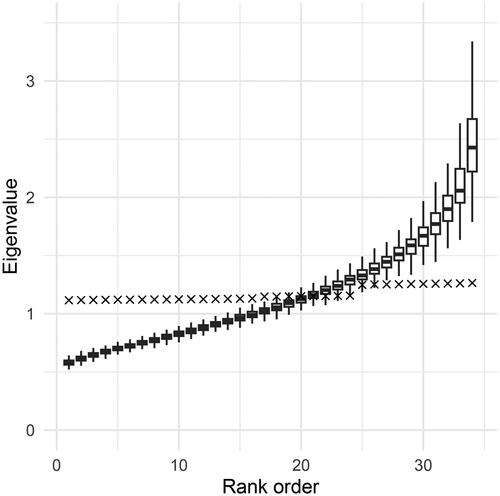(4)(4) $$H(t;l_1,\dots ,l_d)=P\left(\sum _{j=1}^d{l}_j{Z}_j^2>t\right)$$(4) . This procedure is identical to using d blocks (which are then singleton sets) in EBA, and we refer to it as EBAd. Since EBAd has not yet been studied in the literature, it is included in our Monte Carlo investigations. The estimated eigenvalues will converge toward their population counterparts as the sample size increases, so EBAd is asymptotically exact. The sampling variability of estimated eigenvalues is, however, so large that impractical sample sizes may be required to obtain acceptable Type I error control. Figure 1 illustrates the final sample fluctuations in the estimated eigenvalues in a ten-dimensional two-factor model with non-normal data. The model has 34 degrees of freedom, and hence 34 associated non-zero eigenvalues. In the figure, the crosses represented the population values, i.e., the eigenvalues of $U\Gamma ,$ in increasing order, with a range $1.12\text{‐‐}1.27.$ We simulated 200 samples of size n = 1500 and extracted in each sample the sorted eigenvalues of $\widehat{U}\widehat{\Gamma }.$ For each rank $i=1,\dots ,34,$ the corresponding estimated eigenvalues are represented by box plots. We make the following observations: (i) The estimates have high sampling variability, especially the largest eigenvalues. (ii) The higher eigenvalues are consistently overestimated, and the lower eigenvalues are consistently underestimated. (iii) Most of the box plots do not cover their corresponding population eigenvalue. These observations suggest that directly using the estimated eigenvalues to approximate the sampling distribution of $T_{\text{NT}}$ may not work well. While both the SB and the EBA procedures attempt to handle the sampling variability of eigenvalues by averaging sets of eigenvalues, earlier literature has not addressed the problem of under- and overestimation. The new approaches proposed below take the systematic bias into account and are designed to work well when the eigenvalues are related to the true eigenvalues in the same way as in Figure 1.

Figure 1. Population and estimated eigenvalues for a ten-dimensional CFA with 34 degrees of freedom. The × represent population eigenvalues, while the boxplots represent estimated eigenvalues across 200 replications at sample size n = 1500.

Before we turn to the new estimation methods, we explain why the pattern shown in Figure 1 is expected to occur also in conditions not covered by our Monte Carlo study.

1.4. Estimated Eigenvalues and the Empirical Spectral Function

The set of eigenvalues of a matrix are not ordered in and of themselves, although we can naturally sort the eigenvalues in increasing order. What are the statistical consequences of this ordering?

To build intuition, let us consider a highly simplified scenario where the eigenvalue estimates are independent and normal. We observe the set $$S=\{X_1,\dots ,X_d\},\hspace{1em}d=34$$ where $X_1,\dots ,X_d$ are independent, $X_1,\dots ,X_{25}\sim N(2.5,1),$ and $X_{26},\dots ,X_{34}\sim N(3.5,1).$ Although there is an order to the observations in our notation, we only observe the unordered set S, which plays the role of the estimated eigenvalues. This emulates a situation where $U\Gamma$ has 34 eigenvalues, each equal to either 2.5 or 3.5.

If we plot the sorted eigenvalues $X_{(1)}\le X_{(2)}\le \cdots X_{(d)}$ against their rank $(i/d,X_{(i)})$ and connect these points via straight lines, the resulting curve is the empirical quantile function of the data. This curve will approximate the population quantile function. To see why, recall first that the empirical quantile function is a generalized inverse of the empirical distribution function (6) $$\widehat{F}(x)=\frac{1}{d}\sum _{i=1}^{d}I\{X_i\le x\}$$(6) where $I\left\{A\right\}$ is the indicator function of A, being 1 if A is true and zero otherwise. This empirical distribution function $\widehat{F}$ uniformly approximate $\overline{F}(x)=E\widehat{F}(x)$ (Shorack and Wellner, 2009, Chapter 25). Under the assumed distribution for $X_1,\dots ,X_{34},$ we get $\overline{F}(x)=\frac{25}{34}\Phi (x-2.5)+\frac{9}{34}\Phi (x-3.5).$ The empirical quantile function will therefore approximate the inverse of $\overline{F},$ which we may denote by Q(p). Therefore, a plot of $(i/d,X_{(i)})$ will be close to $(i/d,Q(i/d)).$

Figure 2 is based on a single realization of $X_1,\dots ,X_{34}.$ The quantile function Q is plotted in red, the plot of $(i/p,X_{(i)})$ in black, and the empirical quantile function in blue. The black curve is not visible as it is overwritten by the blue curve. Figure 2 displays shapes similar to the eigenvalues plotted in Figure 3. There is systematic over- and underestimation of these values for i/d near zero or one, an effect that is due solely to sorting.

Figure 2. The sorted simulated data plotted against i/d for $i=1,2,\dots ,d.$ the curve in red is the theoretical quantile function. The curve in blue is the empirical quantile function. The dotted black values are the levels of the observations.

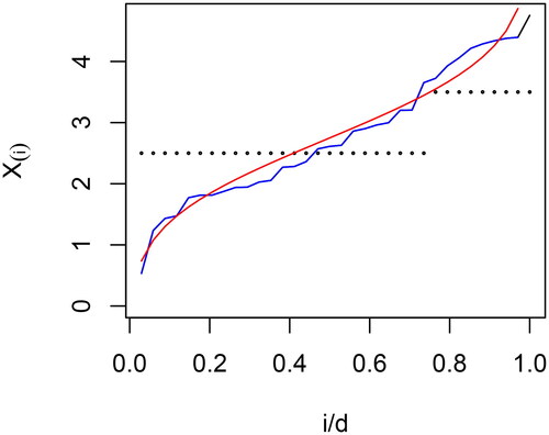
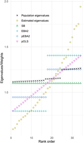
Figure 3. Estimated eigenvalues and associated weights for EBA and regression procedures. EBA2 = 2-block EBA, pEBA2 = penalized 2-block EBA, pOLS = penalized regression, SB = Satorra–Bentler.

While the estimated eigenvalues $({\widehat{\lambda }}_i)$ converge to λ_i, the variation in $({\widehat{\lambda }}_i)$ will be considerable for realistic sample-sizes. A plot of $(i/d,{\widehat{\lambda }}_i)$ will have the shape of an empirical quantile curve defined by the same formula as $\widehat{F}$ above (6), but with ${\widehat{\lambda }}_i$ in place of X_i. Such objects are known as empirical spectral functions and play an important role in random matrix theory (Pastur and Shcherbina, 2011; Paul and Aue, 2014). We conjecture that the empirical spectral function of $\widehat{U}\widehat{\Gamma }$ converges to a population function as d and n increases, so there is a limiting curve that plays a similar role as the red curve in Figure 2. With insights into this limit curve, a principled estimation procedure for approximating ${\lambda }_1,\dots ,{\lambda }_d$ could be developed in future work.

1.5. New Goodness-of-Fit Tests Based on Penalized Estimation

In this section, we introduce and motivate new procedures for obtaining p-values based on penalization of the estimated eigenvalues. Technical arguments are deferred to the online supplementary material.

Similar to the EBA procedures, the new tests takes the estimated eigenvalues ${\widehat{\lambda }}_1,\dots ,{\widehat{\lambda }}_d$ as input. From these values, regularized estimates ${\tilde{\lambda }}_1,\dots ,{\tilde{\lambda }}_d$ are produced as next discussed, and these are used to calculate a p-value for the goodness of fit test using H in eq. (4)(4) $$H(t;l_1,\dots ,l_d)=P\left(\sum _{j=1}^d{l}_j{Z}_j^2>t\right)$$(4) : $$H(T_{\text{NT}};{\tilde{\lambda }}_1,\dots ,{\tilde{\lambda }}_d).$$

For illustration, we continue with the eigenvalues associated with the factor model discussed in Section 1.3 (Figure 1), which has 34 degrees of freedom. Here, however, we consider a single random sample of size n = 1500 and the corresponding set of estimated eigenvalues, using Γ_A. These estimates and their corresponding population values are plotted in Figure 3. Also, the figure depicts four sets of approximated eigenvalues: First, the SB eigenvalues are plotted, all with the same value, namely the mean eigenvalue of 1.10. Second, the EBA2 approximations are depicted, with the 17 smallest eigenvalues set at the mean value 0.79 and the 17 largest eigenvalues at the mean value 1.41. The two remaining eigenvalue sets in the figure, pEBA2 and pOLS, are obtained by a process explained in the next two subsections.

1.6. Penalized EBA

The EBA procedure may be modified naturally to counteract the bias observed in Figures 1 and 3. Figure 3 also contains a new set of eigenvalues in the intermediate positions between SB and EBA2, which we call penalized EBA2 and denote by pEBA2. The connection to penalized estimation is explained in the online supplementary material. pEBA2 consists of a two-block set of weights $({\tilde{\lambda }}_j)$ equal to the average of the SB and the EBA2 weights. In Figure 3, the first block of weights contains the mean value of 1.10 and 0.79, which is 0.95. Likewise, the second block has weights equal to the mean of 1.10 and 1.41, namely 1.26.

The procedure may be performed in the same manner for any number of blocks. That is, we average the EBA weights block by block with the overall average eigenvalue and thus obtain penalized versions pEBA3, pEBA4, and so forth.

The additional averaging employed in penalized EBA attempts to counteract the systematic bias observed in Figures 1 and 3. By anchoring the EBA eigenvalues closer to the global average, the overestimation for the larger eigenvalue estimates is reduced, while still not restricting the eigenvalues to be constant. Similarly, the underestimation of the smaller eigenvalue estimates is also reduced.

1.7. Penalized OLS

The penalized OLS procedure can be motivated by a simple heuristic. Let $({\lambda }_i)$ be the population eigenvalues and run a simple linear regression based on ${(i,{\lambda }_i)}_{i=1}^d$ to obtain the OLS estimates ${\widehat{\beta }}_0$ and ${\widehat{\beta }}_1.$ The ith eigenvalue – which is positive since $U\Gamma$ is positive definite – can now be approximated by ${\tilde{\lambda }}_i=\mathrm{\text{max}}({\beta }_0+{\beta }_{1}i,0).$ This linear approximation inherits the systematic bias observed in Figures 1 and 3, causing the slope to be overestimated. A natural remedy to this sort of overestimation is to down-weight the regression slope using ridge regression, a well-known penalized form of OLS, which we refer to as pOLS.

The extent of down-weighting is represented by a parameter $\gamma >1$ that is applied to the OLS slope parameter β₁: (7) $${\beta }_1(\gamma )=\frac{1}{\gamma }{\beta }_1.$$(7)

The corresponding ridge regression intercept is (8) $${\beta }_0(\gamma )=\overline{\lambda }-{\beta }_1(\gamma ){\overline{i}}_d,\hspace{1em}{\overline{i}}_d:=d^{-1}\sum _{i=1}^{d}i=(d+1)/2.$$(8)

The standard OLS estimates are recovered when γ = 1. For $\gamma \to \infty ,$ we obtain ${\beta }_1=0$ and ${\beta }_0=\overline{\lambda },$ or the Satorra–Bentler weights. Simulations show that γ = 2 works well, and we will use it in the remainder of the article. Figure 3 shows the predictions of pOLS.

1.8. RMSEA with Eigenvalue-Based Tests

The RMSEA is a popular measure of approximate fit originating from the work of Steiger (1990). Using the Satorra–Bentler method, Li and Bentler (2006) found the formula $$\text{RMSEA}=\sqrt{\mathrm{\text{max}}\left(0,d^{-1}\left[T_{\text{NT}}-\frac{\sum _{i=1}^d{\lambda }_i}{N-1}\right]\right)}.$$

Here λ_i are replaced by estimated values in practice. In the online supplementary material, it is shown the proposed penalized eigenvalue-based estimators have the same sum as the Satorra–Bentler estimate, and that the above formula for the RMSEA also holds for these procedures.

2. Monte Carlo Simulation

We considered a two-factor model $x=\Lambda f+ϵ$ where $x=(x_1,\dots ,x_p)\prime$ is a p-dimensional vector of observed variables, $f$ is a two-dimensional latent vector, and $ϵ$ is a p-dimensional vector of uncorrelated residuals, which is also uncorrelated with $f.$ The model had simple structure, with $x_1,\dots ,x_{p/2}$ loading on the first factor and $x_{p/2+1},\dots ,x_p$ loading on the second factor. We included three model sizes with $p=10,20,$ and 40, and corresponding degrees of freedom $d=34,169,$ and 739. This study was not preregistered. The model specifications are available at https://osf.io/6trwu/, together with a database of eigenvalues for each replicated dataset in the present study. The eigenvalues are given for both the biased and the unbiased Γ estimators. The database also contains $T_{\text{ML}}$ and $T_{\text{RLS}}$ and may be used for fast assessment of new variants of eigenvalue-based procedures.

2.1. Population Model

To represent a realistic scenario, we used heterogeneous factor loadings with standardized loadings uniformly drawn in the range $[.3,.8].$ Such loadings reflect values typically found in empirical studies (Li, 2016). The residual variances were then chosen to ensure that the observed variables had unit variance. The factor loadings were nested between models, e.g., for p = 20 the first five loadings for each factor were equal to the corresponding loadings in the p = 10 model. The interfactor correlations in all models were set to .5. For p = 10, the 45 correlations in the observed variables ranged from .08 to .56. For p = 20 the 190 correlations ranged from .08 to .64. The 780 correlations in the p = 40 model ranged from .045 to .64.

2.2. Data Distributions

For each population model, data were drawn from seven distributions. The distributions consisted of the normal distribution and six non-normal distributions. Three of the non-normal distributions had moderate marginal skewness and kurtosis (Curran et al., 1996) taking values 3 and 7, and the other three had severe marginal skewness and kurtosis (with values 3 and 21). We crossed the two marginal non-normality levels with three data distributions: The independent generator (IG) distribution (Foldnes and Olsson, 2016), the piece-wise linear (PL) distribution (Foldnes and Grønneberg, 2021), and the well-known Vale–Maurelli (VM) distribution (Vale and Maurelli, 1983). We use the notation VM1 and VM2 for the VM distributions with the moderate and severe levels of marginal skewness and kurtosis, and similarly for the IG and PL distributions.

Including several classes of non-normal distributions was necessary for the external validity of the study, and was also required for investigating test performance while controlling for marginal skewness and kurtosis. However, note that even with the same skewness and kurtosis, the IG, PL, and VM distributions are different.

2.3. Sample Size

We generated data at sample sizes $n=400,800,1500,$ and 3000, to reflect a range of sample sizes routinely used in empirical investigations.

2.4. Goodness-of-Fit Tests

All test statistics were calculated from normal-theory ML estimates. For the robustified tests and EBAd we considered four candidates, obtained by combining base statistic ($T_{\text{ML}}$ or $T_{\text{RLS}}$) and estimator of the asymptotic covariance matrix (${\widehat{\Gamma }}_{\mathrm{A}}$ or ${\widehat{\Gamma }}_{\mathrm{U}}$).

A total of 43 test statistics were evaluated, including the base statistics $T_{\text{ML}}$ or $T_{\text{RLS}}.$ For the robustified tests we included the traditional tests $T_{\text{SB}}$ and $T_{\text{SS}}$ (a total of 8 candidates), the EBA procedures EBA2, EBA4, and EBA6 (12 candidates), the penalized EBA procedures pEBA2, pEBA4, and pEBA6 (12 candidates), and the pOLS test (4 candidates). Among the asymptotically exact tests, we included the Bollen–Stine bootstrap based on $T_{\text{ML}},$ and the EBA procedure with singleton blocks, EBAd (4 candidates).

2.5. Data Generation and Analysis

Crossing model size, distribution, and sample size resulted in 84 ($3·7·4)$ simulation conditions. We generated 3000 datasets for each condition. All tests except Bollen–Stine were evaluated in each condition based on 3000 replications. The computationally expensive Bollen–Stine test was computed only for n = 800 and n = 3000, and in the largest dimension (p = 40) the number of bootstrap replications was reduced to 1000.

All models were estimated using the maximum likelihood estimator in lavaan (Rosseel, 2012). The package covsim (Grønneberg et al., 2022) was used to simulate from the IG and PL distributions and the package lavaan was used to simulate VM distributions. The goodness-of-fit p-values were calculated using the newly developed package semTests. The package CompQuadForm (Duchesne and De Micheaux, 2010) computed the p-values of the type given in Eq. (3)(3) $${\widehat{p}}_{\text{EBA}2}=H(T_{\text{NT}};{\tilde{\lambda }}_1,\dots ,{\tilde{\lambda }}_d),$$(3) .

2.6. Evaluation Criteria

We employed three evaluation criteria based on the observed percentage rejection rates (RR), obtained in each of the 84 conditions as the percentage of p-values below .05. Hence, we adopted the commonly used significance value of $\alpha =5\%.$

Our first criterion is the root-mean-square error (RMSE), which is a measure of the discrepancy between the observed rejection rate RR and the nominal 5% rejection rate: $\text{RMSE}=\sqrt{\sum _c{(R{R}_c-5)}^2/C},$ where C denotes the number of conditions we are interested in. For instance, if we look at the smallest model size, and we include all distributions and sample sizes, $C=7·4=28.$ Our second criterion, the mean absolute deviation (MAD), is also a measure of the difference between the empirical rejection rates and the nominal rejection rate, defined as $\text{MAD}=\sum _c(|R{R}_c-5|)/C.$

Our third criterion yields the percentage of acceptable rejection rates (ARR), defined as the proportion of conditions c for which $2.5\%<R{R}_c<7.5\%,$ (Bradley, 1978).

Given the large number of test candidates under evaluation, in addition to reporting these three criteria, we also sort the tests according to their RMSE performance in many of our result tables. We acknowledge that the sorting shifts the order of test statistics between tables, making it more difficult to compare the performance of a given test candidate across conditions. However, the sorting greatly facilitates the identification of the best-performing tests by inspecting the upper part of the result tables.

3. Results

3.1. ML, RLS and Robustified Tests

We evaluated two tests based on normality, either with ML and RLS, and 38 robustified tests.

3.1.1. Normal data

Type I error rates in the 12 conditions with normal data are presented in Table 1. For each model size, we have sorted the test statistics according to increasing RMSE values across the four sample sizes. At the smallest model size, p = 10, the normal-theory statistics $T_{\text{ML}}$ and $T_{\text{RLS}}$ performed well, as expected. All 40 test candidates had acceptable rejection rates, ARR = 1, at all sample sizes. The MAD ranged from 0.3% for ML to 0.733% for ${\text{EBA}4}_{\text{RLS}}^{\text{UG}}.$

Table 1. Type I Error rates, normal data.

p = 10					p = 20					p = 40
	n					n					n
Test	400	800	1500	3000	Test	400	800	1500	3000	Test	400	800	1500	3000
$\text{ML}$	4.8	5.7	4.8	5.2	$\text{RLS}$	5.4	4.9	5.4	4.7	${\text{SB}}_{\text{RLS}}^{\text{UG}}$	4.8	4.5	4.8	4.5
$\text{SB}$	4.7	5.8	4.8	5.2	${\text{SB}}_{\text{RLS}}^{\text{UG}}$	4.8	4.7	5.4	4.6	$\text{RLS}$	6.2	5.3	5.0	4.5
$\text{RLS}$	4.4	5.6	4.6	4.9	${\text{pEBA}2}_{\text{RLS}}$	4.8	4.7	5.4	4.6	${\text{pEBA}2}_{\text{RLS}}$	4.5	4.0	4.5	4.3
${\text{SB}}^{\text{UG}}$	4.4	5.7	4.8	5.1	${\text{SB}}_{\text{RLS}}$	5.6	5.1	5.5	4.7	${\text{SB}}_{\text{RLS}}$	6.8	5.5	5.2	4.6
$\text{pEBA}2$	4.4	5.7	4.8	5.2	${\text{pOLS}}_{\text{RLS}}$	4.5	4.5	5.3	4.5	${\text{pEBA}2}_{\text{UG}}$	5.4	3.7	4.2	3.8
$\text{pEBA}4$	4.4	5.7	4.8	5.2	${\text{pEBA}4}_{\text{RLS}}$	4.5	4.5	5.4	4.5	${\text{pOLS}}_{\text{RLS}}$	3.4	3.3	4.2	4.0
$\text{pEBA}6$	4.4	5.7	4.8	5.2	${\text{pEBA}6}_{\text{RLS}}$	4.4	4.5	5.3	4.5	${\text{pEBA}4}_{\text{RLS}}$	3.3	3.3	4.3	4.0
$\text{pOLS}$	4.4	5.7	4.8	5.2	$\text{EBA}2$	5.0	4.1	5.3	4.6	${\text{pEBA}2}_{\text{RLS}}^{\text{UG}}$	3.3	3.2	4.2	4.0
${\text{pEBA}4}^{\text{UG}}$	4.2	5.6	4.7	5.1	${\text{pEBA}4}^{\text{UG}}$	5.9	4.7	5.6	4.8	$\text{EBA}2$	7.5	4.4	4.4	4.0
${\text{pEBA}6}^{\text{UG}}$	4.2	5.6	4.7	5.1	${\text{pEBA}6}^{\text{UG}}$	5.9	4.7	5.6	4.8	${\text{pEBA}6}_{\text{RLS}}$	3.1	3.2	4.2	4.0
${\text{pOLS}}^{\text{UG}}$	4.2	5.6	4.7	5.1	${\text{pOLS}}^{\text{UG}}$	5.9	4.7	5.6	4.8	$\text{EBA}4$	3.1	2.5	3.6	3.6
${\text{pEBA}2}^{\text{UG}}$	4.2	5.6	4.7	5.1	${\text{pEBA}2}_{\text{RLS}}^{\text{UG}}$	4.1	4.3	5.3	4.5	${\text{pOLS}}_{\text{RLS}}^{\text{UG}}$	2.5	2.7	3.7	3.7
${\text{SB}}_{\text{RLS}}$	4.4	5.9	4.6	5.1	${\text{pEBA}2}^{\text{UG}}$	6.1	5.0	5.7	4.8	${\text{pEBA}4}_{\text{RLS}}^{\text{UG}}$	2.4	2.6	3.8	3.7
$\text{EBA}2$	4.1	5.4	4.5	5.1	${\text{pEBA}2}_{\text{UG}}$	4.2	3.8	5.2	4.5	${\text{pEBA}6}_{\text{RLS}}^{\text{UG}}$	2.1	2.4	3.7	3.7
${\text{pEBA}2}_{\text{RLS}}$	4.1	5.7	4.6	5.0	${\text{pEBA}4}_{\text{RLS}}^{\text{UG}}$	3.8	4.1	5.2	4.5	$\text{EBA}6$	2.4	2.3	3.3	3.5
${\text{pEBA}4}_{\text{RLS}}$	4.1	5.7	4.6	4.9	${\text{pOLS}}_{\text{RLS}}^{\text{UG}}$	3.8	4.0	5.2	4.4	${\text{EBA}4}^{\text{UG}}$	2.2	2.2	3.2	3.4
${\text{pEBA}6}_{\text{RLS}}$	4.0	5.7	4.6	4.9	${\text{pEBA}6}_{\text{RLS}}^{\text{UG}}$	3.8	4.0	5.2	4.4	$\text{SS}$	2.0	2.2	3.3	3.5
${\text{SB}}_{\text{RLS}}^{\text{UG}}$	4.0	5.7	4.6	4.9	$\text{pEBA}6$	6.6	5.3	5.7	4.8	${\text{pEBA}6}^{\text{UG}}$	9.6	6.4	5.3	4.7
${\text{pOLS}}_{\text{RLS}}$	4.0	5.7	4.6	4.9	$\text{EBA}4$	4.0	3.6	5.2	4.5	${\text{EBA}6}^{\text{UG}}$	1.8	2.1	3.0	3.2
${\text{pEBA}2}_{\text{RLS}}^{\text{UG}}$	3.8	5.5	4.6	4.9	$\text{pOLS}$	6.7	5.3	5.7	4.8	${\text{SS}}^{\text{UG}}$	1.5	2.0	2.8	3.2
$\text{EBA}4$	3.8	5.4	4.4	5.0	$\text{pEBA}4$	6.7	5.3	5.8	4.8	${\text{EBA}2}_{\text{RLS}}$	1.4	1.6	2.8	3.1
$\text{SS}$	3.8	5.4	4.4	5.0	$\text{SS}$	3.8	3.6	5.2	4.5	${\text{pEBA}4}^{\text{UG}}$	10.4	6.8	5.5	4.7
${\text{pEBA}2}_{\text{UG}}$	3.8	5.4	4.3	5.0	$\text{EBA}6$	3.8	3.5	5.1	4.5	${\text{pOLS}}^{\text{UG}}$	10.9	6.9	5.5	4.7
$\text{EBA}6$	3.8	5.4	4.3	5.0	${\text{EBA}4}^{\text{UG}}$	3.6	3.3	5.0	4.4	${\text{EBA}2}_{\text{RLS}}^{\text{UG}}$	1.0	1.3	2.6	3.0
${\text{pEBA}4}_{\text{RLS}}^{\text{UG}}$	3.7	5.5	4.5	4.8	$\text{pEBA}2$	7.1	5.4	5.8	4.9	${\text{EBA}4}_{\text{RLS}}$	0.4	1.1	2.3	2.9
${\text{pEBA}6}_{\text{RLS}}^{\text{UG}}$	3.7	5.5	4.5	4.8	${\text{SB}}^{\text{UG}}$	7.2	5.4	5.8	4.9	${\text{EBA}6}_{\text{RLS}}$	0.3	0.9	2.2	2.9
${\text{pOLS}}_{\text{RLS}}^{\text{UG}}$	3.7	5.5	4.5	4.8	${\text{SS}}^{\text{UG}}$	3.5	3.3	5.0	4.4	${\text{SS}}_{\text{RLS}}$	0.2	0.8	2.2	2.9
${\text{EBA}2}_{\text{RLS}}$	3.6	5.4	4.5	4.8	${\text{EBA}6}^{\text{UG}}$	3.5	3.3	5.0	4.4	${\text{EBA}4}_{\text{RLS}}^{\text{UG}}$	0.2	0.8	2.1	2.8
${\text{SS}}^{\text{UG}}$	3.6	5.3	4.3	4.9	${\text{EBA}2}_{\text{RLS}}$	3.2	3.3	4.9	4.3	${\text{EBA}6}_{\text{RLS}}^{\text{UG}}$	0.2	0.7	1.9	2.7
${\text{EBA}4}_{\text{RLS}}$	3.5	5.3	4.5	4.7	${\text{EBA}2}_{\text{RLS}}^{\text{UG}}$	2.8	3.1	4.7	4.2	${\text{SS}}_{\text{RLS}}^{\text{UG}}$	0.2	0.7	1.9	2.7
${\text{SS}}_{\text{RLS}}$	3.5	5.3	4.5	4.7	$\text{ML}$	7.8	5.9	6.0	5.0	$\text{pEBA}6$	12.4	7.6	5.9	4.8
${\text{EBA}4}^{\text{UG}}$	3.6	5.3	4.3	4.9	${\text{EBA}4}_{\text{RLS}}$	2.4	3.0	4.7	4.2	${\text{pEBA}2}^{\text{UG}}$	13.0	7.6	5.8	4.8
${\text{EBA}2}_{\text{RLS}}^{\text{UG}}$	3.5	5.3	4.4	4.7	$\text{SB}$	8.0	6.0	6.1	5.0	$\text{pEBA}4$	13.2	7.8	6.0	4.8
${\text{EBA}6}_{\text{RLS}}$	3.5	5.3	4.4	4.7	${\text{SS}}_{\text{RLS}}$	2.3	3.0	4.7	4.2	$\text{pOLS}$	14.0	7.8	5.9	4.8
${\text{EBA}6}^{\text{UG}}$	3.5	5.3	4.3	4.9	${\text{EBA}6}_{\text{RLS}}$	2.3	3.0	4.7	4.1	$\text{pEBA}2$	16.4	8.7	6.4	4.8
${\text{SS}}_{\text{RLS}}^{\text{UG}}$	3.3	5.2	4.3	4.7	${\text{EBA}4}_{\text{RLS}}^{\text{UG}}$	2.0	2.8	4.4	4.1	${\text{SB}}^{\text{UG}}$	17.5	9.8	7.0	5.1
${\text{EBA}4}_{\text{RLS}}^{\text{UG}}$	3.3	5.1	4.3	4.6	${\text{SS}}_{\text{RLS}}^{\text{UG}}$	1.8	2.8	4.4	4.1	$\text{ML}$	20.2	10.5	7.4	5.3
${\text{EBA}6}_{\text{RLS}}^{\text{UG}}$	3.3	5.1	4.3	4.6	${\text{EBA}6}_{\text{RLS}}^{\text{UG}}$	1.8	2.8	4.4	4.1	$\text{SB}$	21.6	11.1	7.4	5.3

Within each dimension, the tests are sorted according to increasing RMSE.

With increasing model size, test performance generally deteriorated, as expected. Especially striking was the poor performance of ML in comparison to RLS. For instance, for p = 20 and p = 40 the MAD of ML was 1.18% and 5.85%, respectively. In comparison, the MAD of RLS was negligible for p = 20 and p = 40: 0.29% and 0.51%, respectively. Also, for dimensions p = 20 and p = 40 the robustified test ${\text{SB}}_{\text{RLS}}^{\text{UG}}$ was a top performer. Indeed, this test was the overall winner in terms of RMSE when collapsed over all 12 conditions, with RLS as the runner-up.

3.1.2. Non-Normal Data

Type I error rates for all tests in the 12 conditions (3 models, 4 sample sizes) are tabulated for each non-normal distribution in the supplementary material, see Tables B2–B7. In Table 2 we report aggregated results over the six non-normal distributions. Test performance was calculated for each model size, across six distributions and four sample sizes, and test candidates were ranked according to increasing RMSE.

Table 2. Test performance across 6 non-normal distributions and 4 sample sizes, ranked in increasing RMSE order.

p = 10				p = 20				p = 40
Test	RMSE	MAD	ARR	Test	RMSE	MAD	ARR	Test	RMSE	MAD	ARR
${\text{pOLS}}^{\text{UG}}$	0.63	0.54	100.0	${\text{pOLS}}_{\text{RLS}}$	1.25	0.93	87.5	${\text{pEBA}4}_{\text{RLS}}$	1.44	1.31	95.8
${\text{pOLS}}_{\text{RLS}}$	0.64	0.53	100.0	${\text{pEBA}4}_{\text{RLS}}$	1.25	0.96	91.7	${\text{pEBA}4}_{\text{RLS}}^{\text{UG}}$	1.66	1.46	83.3
$\text{pOLS}$	0.64	0.55	100.0	${\text{pOLS}}_{\text{RLS}}^{\text{UG}}$	1.30	1.06	91.7	${\text{pOLS}}_{\text{RLS}}$	1.71	1.52	87.5
${\text{pEBA}2}_{\text{RLS}}^{\text{UG}}$	0.65	0.54	100.0	${\text{pEBA}6}_{\text{RLS}}$	1.30	1.11	95.8	${\text{pEBA}6}_{\text{RLS}}$	1.76	1.55	87.5
$\text{pEBA}6$	0.65	0.56	100.0	${\text{pEBA}4}_{\text{RLS}}^{\text{UG}}$	1.30	1.08	91.7	${\text{pEBA}2}_{\text{RLS}}^{\text{UG}}$	1.80	1.29	83.3
${\text{pEBA}4}^{\text{UG}}$	0.65	0.56	100.0	${\text{pEBA}6}_{\text{RLS}}^{\text{UG}}$	1.45	1.25	95.8	${\text{pOLS}}_{\text{RLS}}^{\text{UG}}$	2.14	1.94	70.8
${\text{pEBA}4}_{\text{RLS}}$	0.66	0.54	100.0	${\text{pEBA}2}_{\text{RLS}}^{\text{UG}}$	1.46	1.02	87.5	${\text{pEBA}6}_{\text{RLS}}^{\text{UG}}$	2.16	2.00	70.8
$\text{pEBA}4$	0.66	0.57	100.0	${\text{pEBA}4}^{\text{UG}}$	1.61	1.31	87.5	${\text{EBA}2}_{\text{RLS}}$	2.34	2.13	41.7
${\text{pEBA}2}_{\text{RLS}}$	0.67	0.57	100.0	${\text{pOLS}}^{\text{UG}}$	1.63	1.30	87.5	${\text{pEBA}6}^{\text{UG}}$	2.58	2.17	54.2
${\text{pEBA}2}^{\text{UG}}$	0.68	0.58	100.0	${\text{pEBA}6}^{\text{UG}}$	1.64	1.42	83.3	${\text{EBA}2}_{\text{RLS}}^{\text{UG}}$	2.62	2.41	37.5
${\text{pEBA}6}_{\text{RLS}}$	0.69	0.57	100.0	$\text{pEBA}6$	1.66	1.36	87.5	${\text{pOLS}}^{\text{UG}}$	2.62	2.20	54.2
${\text{pEBA}6}^{\text{UG}}$	0.70	0.57	100.0	${\text{pEBA}2}_{\text{RLS}}$	1.72	1.14	79.2	${\text{pEBA}2}_{\text{UG}}$	2.63	2.37	45.8
${\text{pOLS}}_{\text{RLS}}^{\text{UG}}$	0.72	0.60	100.0	$\text{pEBA}4$	1.77	1.27	87.5	$\text{EBA}2$	2.76	2.32	62.5
${\text{pEBA}4}_{\text{RLS}}^{\text{UG}}$	0.73	0.61	100.0	$\text{pOLS}$	1.78	1.25	83.3	${\text{pEBA}4}^{\text{UG}}$	2.76	2.14	62.5
${\text{pEBA}6}_{\text{RLS}}^{\text{UG}}$	0.79	0.67	100.0	${\text{EBA}2}_{\text{RLS}}$	1.81	1.68	91.7	${\text{pEBA}2}_{\text{RLS}}$	2.77	1.70	75.0
$\text{pEBA}2$	0.80	0.66	100.0	$\text{EBA}2$	1.81	1.64	87.5	$\text{pEBA}6$	2.95	2.32	58.3
${\text{SB}}_{\text{RLS}}^{\text{UG}}$	0.89	0.72	100.0	${\text{pEBA}2}^{\text{UG}}$	1.97	1.27	83.3	$\text{pOLS}$	3.04	2.33	54.2
${\text{SB}}_{\text{RLS}}$	1.05	0.87	100.0	${\text{pEBA}2}_{\text{UG}}$	1.97	1.80	87.5	${\text{SB}}_{\text{RLS}}^{\text{UG}}$	3.33	2.49	58.3
${\text{SB}}^{\text{UG}}$	1.07	0.86	100.0	${\text{EBA}2}_{\text{RLS}}^{\text{UG}}$	2.02	1.85	75.0	$\text{pEBA}4$	3.55	2.44	58.3
$\text{EBA}2$	1.17	0.93	100.0	${\text{SB}}_{\text{RLS}}^{\text{UG}}$	2.30	1.70	70.8	$\text{EBA}4$	3.75	3.56	20.8
$\text{SB}$	1.30	1.06	100.0	$\text{pEBA}2$	2.31	1.58	75.0	${\text{EBA}4}^{\text{UG}}$	3.92	3.76	16.7
${\text{EBA}2}_{\text{RLS}}$	1.31	1.06	95.8	${\text{SB}}_{\text{RLS}}$	2.84	2.20	62.5	${\text{EBA}4}_{\text{RLS}}$	4.02	3.94	8.3
${\text{pEBA}2}_{\text{UG}}$	1.33	1.08	95.8	${\text{SB}}^{\text{UG}}$	2.92	2.16	66.7	${\text{EBA}4}_{\text{RLS}}^{\text{UG}}$	4.14	4.07	4.2
${\text{EBA}2}_{\text{RLS}}^{\text{UG}}$	1.47	1.21	95.8	$\text{EBA}4$	2.96	2.71	41.7	$\text{EBA}6$	4.16	4.05	12.5
$\text{EBA}4$	1.93	1.69	75.0	${\text{EBA}4}_{\text{RLS}}$	3.08	2.88	37.5	${\text{EBA}6}^{\text{UG}}$	4.26	4.17	4.2
${\text{EBA}4}_{\text{RLS}}$	1.98	1.75	75.0	${\text{EBA}4}^{\text{UG}}$	3.09	2.85	37.5	${\text{pEBA}2}^{\text{UG}}$	4.27	2.78	66.7
${\text{EBA}4}^{\text{UG}}$	2.06	1.82	75.0	${\text{EBA}4}_{\text{RLS}}^{\text{UG}}$	3.21	3.01	25.0	${\text{EBA}6}_{\text{RLS}}$	4.35	4.29	4.2
${\text{EBA}4}_{\text{RLS}}^{\text{UG}}$	2.10	1.88	66.7	$\text{EBA}6$	3.30	3.05	37.5	${\text{EBA}6}_{\text{RLS}}^{\text{UG}}$	4.42	4.37	4.2
$\text{EBA}6$	2.22	1.97	70.8	${\text{EBA}6}^{\text{UG}}$	3.42	3.18	29.2	$\text{SS}$	4.62	4.59	0.0
${\text{EBA}6}_{\text{RLS}}$	2.25	2.02	66.7	${\text{EBA}6}_{\text{RLS}}$	3.43	3.23	25.0	${\text{SS}}^{\text{UG}}$	4.65	4.62	0.0
$\text{SS}$	2.29	2.03	70.8	$\text{SB}$	3.50	2.69	54.2	${\text{SS}}_{\text{RLS}}$	4.72	4.70	0.0
${\text{EBA}6}^{\text{UG}}$	2.33	2.09	66.7	${\text{EBA}6}_{\text{RLS}}^{\text{UG}}$	3.54	3.33	25.0	${\text{SS}}_{\text{RLS}}^{\text{UG}}$	4.74	4.72	0.0
${\text{EBA}6}_{\text{RLS}}^{\text{UG}}$	2.34	2.11	66.7	$\text{SS}$	3.78	3.61	20.8	${\text{SB}}_{\text{RLS}}$	4.76	3.66	45.8
${\text{SS}}_{\text{RLS}}$	2.37	2.13	66.7	${\text{SS}}^{\text{UG}}$	3.85	3.69	20.8	$\text{pEBA}2$	5.82	3.79	58.3
${\text{SS}}^{\text{UG}}$	2.41	2.16	66.7	${\text{SS}}_{\text{RLS}}$	3.88	3.74	20.8	${\text{SB}}^{\text{UG}}$	6.48	4.53	45.8
${\text{SS}}_{\text{RLS}}^{\text{UG}}$	2.45	2.21	62.5	${\text{SS}}_{\text{RLS}}^{\text{UG}}$	3.95	3.81	16.7	$\text{SB}$	8.50	6.08	41.7
$\text{RLS}$	48.84	39.58	0.0	$\text{RLS}$	76.73	69.55	0.0	$\text{RLS}$	79.48	72.15	0.0
$\text{ML}$	49.24	40.10	0.0	$\text{ML}$	77.26	70.48	0.0	$\text{ML}$	80.85	75.33	0.0

RMSE: root mean square error in percentage; MAD: mean absolute deviation of rejection rates from 5%; ARR: percentage of acceptable rejection rates.

Under non-normality, the normal-theory statistics ML and RLS performed poorly. In fact, in none of the 72 non-normal conditions did these tests achieve an acceptable rejection rate.

Expectedly, the normal-theory tests were outperformed by the traditional robustified tests, SB and SS. Generally, SB outperformed SS, and the SB candidate with the consistently best performance was ${\text{SB}}_{\text{RLS}}^{\text{UG}}.$ The standard SB test, which is based on ML and ${\widehat{\Gamma }}_{\mathrm{A}},$ performed remarkably worse than ${\text{SB}}_{\text{RLS}}^{\text{UG}},$ which is based on RLS and ${\widehat{\Gamma }}_{\mathrm{U}}.$ For instance, collapsing over all 72 non-normal conditions, the MAD of SB and ${\text{SB}}_{\text{RLS}}^{\text{UG}}$ was 3.28% and 1.63%, respectively. Also, the ARR of SB was 65.3%, compared to 76.4% for ${\text{SB}}_{\text{RLS}}^{\text{UG}}.$ Among the SS candidates, performance was best when based on ML and ${\widehat{\Gamma }}_{\mathrm{A}}.$ However, even for this candidate, SS, had overall poor performance, especially in the large model, where ARR was zero.

Many candidates in the family of newly developed procedures (EBA, pEBA, and pOLS) outperformed the SB and SS procedures. The RMSE rank in Table 2 of the best traditional robustified test, ${\text{SB}}_{\text{RLS}}^{\text{UG}},$ was 17, 20, and 18 for dimensions 10, 20 and 40, respectively. To further give an overview of the best-performing tests, we aggregated also over model size, with the resulting ten best performers (in terms of RMSE) presented in Table 3. This table hence is based on collapsing 72 conditions (six distributions, four sample sizes, and 3 model sizes). The top nine performers in Table 3 all belong to the new class of penalized eigenvalue modeling. Also noteworthy, eight of the ten tests are based on RLS, and only two on ML.

Table 3. Top ten robustified tests according to RMSE when aggregating 6 non-normal distributions, 4 sample sizes and 3 model sizes.

Test	RMSE	MAD	ARR
${\text{pEBA}4}_{\text{RLS}}$	1.16	0.94	95.8
${\text{pOLS}}_{\text{RLS}}$	1.28	0.99	91.7
${\text{pEBA}4}_{\text{RLS}}^{\text{UG}}$	1.29	1.05	91.7
${\text{pEBA}6}_{\text{RLS}}$	1.32	1.07	94.4
${\text{pEBA}2}_{\text{RLS}}^{\text{UG}}$	1.39	0.95	90.3
${\text{pOLS}}_{\text{RLS}}^{\text{UG}}$	1.50	1.20	87.5
${\text{pEBA}6}_{\text{RLS}}^{\text{UG}}$	1.57	1.31	88.9
${\text{pEBA}6}^{\text{UG}}$	1.81	1.39	79.2
${\text{pOLS}}^{\text{UG}}$	1.82	1.35	80.6
${\text{EBA}2}_{\text{RLS}}$	1.86	1.62	76.4

RMSE: root mean square error in percentage; MAD: mean absolute deviation of rejection rates from 5%; ARR: percentage of acceptable rejection rates.

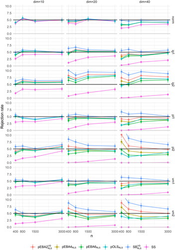
To investigate in full detail the performance of some of the best tests in Table 3, we picked the top candidate from the pEBA2, pEBA4, pEBA6, and pOLS families, namely ${\text{EBA}2}_{\text{RLS}}^{\text{UG}},{\text{pEBA}4}_{\text{RLS}},{\text{pEBA}6}_{\text{RLS}},$ and ${\text{pOLS}}_{\text{RLS}}.$ The rejection rates in all 72 conditions of these four candidates are plotted in Figure 4. The figure also includes the best candidate in each of the traditional families of robustified tests: ${\text{SB}}_{\text{RLS}}^{\text{UG}}$ for SB, and SS for SS. A consistent pattern is that the newly developed tests were associated with rejection rates intermediate between SS, which severely under-rejected, and ${\text{SB}}_{\text{RLS}}^{\text{UG}},$ which tended to over-reject. The figure demonstrates that goodness-of-fit testing was more challenging in larger models, while larger sample sizes are associated with better Type I error control. Also, the distributional type affected the test procedures. Under normality (see also Table 1), all tests performed well, except SS in the largest model. Under non-normality, we see that performance depended on marginal kurtosis, as expected, with overall MAD (across tests, distributions, and model sizes) equal to 1.11% for the skewness = 2, kurtosis = 7 condition (IG1, PL1, VM1) and 1.88% for the skewness = 7, kurtosis = 21 condition (IG2, PL2, VM2). Also, there was some variation in overall test performance among the underlying distributional class. The overall MAD for distributions of type IG, PL, and VM was 1.56%, 1.50%, and 1.43%, respectively.

Figure 4. Rejection rates in % for six selected tests. Panel columns and rows correspond to model size and distribution, respectively.

3.2. Asymptotically Exact Tests

Table 4 presents the Bollen–Stine rejection rates. The underlying distribution strongly affected test performance, with severe overrejection for PL2 and partly for VM2. In the large model, for PL2 and VM2, the rejection rate was virtually 100%, in striking contrast to the finding in Ferraz et al. (2022) that the Bollen–Stine test tended to underreject in a p = 30 model. In contrast, under the normal and IG distributions, Bollen–Stine consistently underrejected, reflecting the findings in Ferraz et al. (2022). Overall, echoing the findings of Ferraz et al. (2022), as model size increased, Bollen–Stine performed poorly, even for n = 3000.

Table 4. Rejection rate in % for the bollen–stine bootstrap.

n	Distribution	p = 10	p = 20	p = 40
800	Normal	4.0	2.5	1.1
	IG1	4.7	3.4	1.1
	IG2	5.6	5.0	1.4
	PL1	4.3	5.8	69.1
	PL2	10.2	93.1	100.0
	VM1	4.7	3.8	12.2
	VM2	6.6	55.2	99.9
3000	Normal	4.5	4.3	2.4
	IG1	4.7	3.8	2.0
	IG2	4.5	5.1	3.4
	PL1	3.7	4.6	64.1
	PL2	10.7	95.5	100.0
	VM1	4.7	4.5	7.6
	VM2	5.4	56.8	100.0

Next, consider the asymptotically exact test EBAd. The differences between the four EBAd candidates were small (see Figure B1 in the supplementary material). Therefore, in Table 5 we only report results for the default version, which is based on ML and ${\widehat{\Gamma }}_{\mathrm{A}}.$ The results are aggregated over all 7 distributions. The test exhibited poor Type I error control, especially at low sample sizes, with severe underrejection. The asymptotic superiority of $\text{EBAd}$ was not yet detectable at sample size n = 3000. To further inspect the rate of converge to nominal 5% rejection rates, and to confirm asymptotic consistency, we simulated some very large sample size conditions ($n={10}^4,{10}^5$). Even at $n={10}^4$ the tendency to underreject was still pronounced for dimensions p = 20 and p = 40. For instance, for p = 40 and $n={10}^4$ the overall rejection rate across distributions was only 2.6%.

Table 5. Rejection rate in % for the $\text{EBAd}$ test procedure, aggregated over all seven distributions.

	n
	400	800	1500	3000	10^4	10^5
p = 10	2.0	2.9	3.0	4.0	4.8	4.9
p = 20	0.8	1.1	1.9	2.6	3.8	4.7
p = 40	0.3	0.4	0.8	1.2	2.6	4.8

4. Illustration of the Package semTests

We demonstrate the use of the newly developed R package semTests (Moss, 2024) by conducting a small power study. Consider the model with p = 20 observed variables used in our Monte Carlo study (see supplementary online material for the complete model specification). We first simulate a n = 800 non-normal data set from this model using the VM2 distribution. Then we run the pvalues() function from semTests on the fitted model, using the default parameter values. The default p-values reported were chosen from the best-performing tests in our Monte Carlo study, in addition to the best-performing traditional test ${\text{SB}}_{\text{RLS}}^{\text{UG}}.$

library(semTests); library(lavaan)

set.seed(1234)

X <- simulateData(m2, sample.nobs = 800,

↪ skewness = 3, kurtosis = 21)

f <- cfa(m2, data = X)

pvals <- pvalues(f)

round(pvals,3)

#sb_ug_rls peba2_ug_rls peba4_rls peba6_rls

↪ pols2_rls

# 0.106 0.125 0.139 0.152 0.144

The reported p-values are similar, with ${\text{SB}}_{\text{RLS}}^{\text{UG}}$ having the smallest p-value.

Next, we conduct a small power study with 1000 replications where n = 800 and data is drawn from a VM2 distribution. Model misspecification is obtained by adding a cross-loading with standardized factor loading of 0.4.

m2_misspecified_pop <- paste(m2, “; F1=∼start

↪ (0.4)*x11”)

simres <- sapply(1:1000, \(i){

set.seed(i)

X <- simulateData(m2_misspecified_pop,

↪ sample.nobs = 800, skewness = 3, kurtosis

↪ =21)

f <- cfa(m2, data = X)

pvalues(f)})

rowMeans(simres < .05)

#sb_ug_rls peba2_ug_rls peba4_rls peba6_rls

↪ pols2_rls

# 0.705 0.666 0.624 0.598 0.631

The rejection rates are ordered in the same way as observed for the Type I errors in Figure 4 (see bottom middle panel at n = 800). Highest power is achieved by ${\text{SB}}_{\text{RLS}}^{\text{UG}},$ which also had the highest rejection rate, 7.1%, among the tests in Figure 4. Hence, in terms of power, ${\text{SB}}_{\text{RLS}}^{\text{UG}}$ outperformed the other test candidates. However, Type I error control is a more fundamental requirement than adequate power, and the other test candidates outperform ${\text{SB}}_{\text{RLS}}^{\text{UG}}$ in terms of Type I error control.

5. Discussion

We have proposed and evaluated new goodness-of-fit methods for factor analysis and structural equation modeling with non-normal data. The new methods pEBA and pOLS apply penalization on the estimated eigenvalues of $U\Gamma .$ The pEBA methods were derived from the EBA approach (Foldnes and Grønneberg, 2017) and the pOLS methods are based on a linear approximation of the sorted eigenvalues, where the penalization is obtained by dampening the slope. We have provided a formal analysis of eigenvalue modeling that motivates pEBA and pOLS.

In the past, many tests have been proposed to handle goodness-of-fit testing under non-normality, and we conducted a large Monte Carlo study to compare the Type I error control of the new methods with well-known traditional tests such as the Satorra–Bentler scaled test, the scaled and shifted test, and the Bollen–Stine bootstrap test. Moreover, we took recent developments into account by acknowledging that the little-known normal-theory RLS test (Browne, 1974) might outperform the classical normal-theory ML test in multivariate normal conditions, and that replacing the traditionally used asymptotically unbiased Γ estimator ${\widehat{\Gamma }}_{\mathrm{A}}$ by an unbiased estimator ${\widehat{\Gamma }}_{\mathrm{U}}$ might improve test performance. Therefore, the Monte Carlo study evaluated four versions (ML/RLS, ${\widehat{\Gamma }}_{\mathrm{U}}$/${\widehat{\Gamma }}_{\mathrm{A}}$) of each test statistic.

5.1. Practical Recommendations

For the special case of normal data, our results echoed earlier findings (e.g., Hayakawa, 2019) in demonstrating that the RLS test is far superior to the more commonly used ML test. Therefore, we advise using $T_{\text{RLS}}$ instead of $T_{\text{ML}}$ when reporting goodness-of-fit in normal data conditions.

For non-normal data, our recommendations are as follows. Echoing Ferraz et al., 2022, we do not recommend using the Bollen–Stine bootstrap test. This test is computationally heavy and was found to adequately control Type I error only in the smallest model with 10 observed variables, and then only for five of the six non-normal conditions. In a model with 40 observed variables, we found the bootstrap test to perform poorly even with a sample size of 3000.

For the Satorra–Bentler test, we demonstrated an improved Type I error control by applying the scaling to the RLS test statistic instead of the commonly used ML statistic. Furthermore, performance is improved by replacing ${\widehat{\Gamma }}_{\mathrm{A}}$ by ${\widehat{\Gamma }}_{\mathrm{U}}$ when calculating the scaling factor. As in previous studies (e.g., Foldnes and Olsson, 2015), the scaled-and-shifted test was found to perform poorly with severe under-rejection in most conditions, and we discourage its use unless the sample size is very large.

Overall, the nine best-performing tests in our Monte Carlo study all were of pEBA or pOLS type. Based on Table 3, we recommend basing goodness-of-fit in non-normal conditions on ${\text{pEBA}4}_{\text{RLS}}$ or ${\text{pOLS}}_{\text{RLS}}.$

5.2. Limitations and Future Research

We have focused exclusively on continuous data. However, the methods we propose are naturally applicable to ordinal data analyzed using polychoric correlations. It is natural to ask whether pEBA and pOLS outperform the currently available methods in the testing of ordinal factor models, such as the SS test used by lavaan (Rosseel, 2012).

The idea of eigenvalue penalization has not been fully explored yet, and different variants could potentially result in better test performance. A more thorough analysis of eigenvalue modeling could shed more light on the subject. Using uneven block sizes in the pEBA is another possibility. Future estimation of the eigenvalues could also be based on the limiting behavior of the spectral distribution of $\widehat{U}\widehat{\Gamma }.$

A natural extension of the present paper is to consider power. That is, among tests that control Type I error, which candidate best detects model misspecification? We consider this as a topic for a future Monte Carlo study. The results of such a study must involve balancing the primary concern of Type I error control with the secondary concern of power.

Our Monte Carlo design is limited in several ways. We only considered factor analysis models, not more general structural equation models. Moreover, the number of observed variables ranged from 10 to 40, but models with hundreds of observed variables are not uncommon in applied research. A study of about 50–100 variables would shed more light on such situations. We modeled three types of non-normal distributions, across two conditions of marginal non-normality as measured in terms of marginal skewness and kurtosis. But other kinds of non-normality is certainly encountered in practice, and further research could be conducted by employing more flexible non-normal distributional classes such as the flexible VITA method suggested by Grønneberg and Foldnes, 2017 and implemented in the R package covsim (Grønneberg et al., 2022). Finally, we considered model fit only for non-nested models. Nested model testing is widely conducted in measurement invariance testing, and the new test procedures can naturally be applied also in these situations.

6. Conclusion

We have proposed several new methods for evaluating model fit of structural equation models and evaluated their performance in a Monte Carlo study of factor models. The new methods outperform existing methods such as Satorra–Bentler in terms of Type I error control. The overall best-performing test, ${\text{pEBA}4}_{\text{RLS}},$ performed adequately in 69 of 72 non-normal conditions. The new methods are available in the R package semTests.