Standing on the shoulders of giants. Paternal life course effects on son’s heights outcomes in the Netherlands 1820-1960

ABSTRACT

This article aims to answer the question: what makes you taller than your father? To study this intergenerational growth, conscription heights from the Historical Sample of the Netherlands are used from the period 1820–1960. A growth estimation method on the individual level is introduced to cope with the variance in growth windows in the nineteenth century, especially to estimate growth after conscription. Both the influence of external and household factors are examined. Moreover, the external living conditions of the mother are included in the analyses as well. It was found that the disease environment, proxied by crude death rates, affects heights within a generation and so an improvement in these conditions makes a son taller. What adds to this is that maternal early life conditions play a crucial role in outgrowing a father if these conditions differ from that of the father himself. Furthermore, sibship size was found to have a negative effect on heights. Furthermore, social mobility achieved by the father was associated with a larger height difference with his son. Still, on average, sons did not yet reach the heights of higher socioeconomic peers after paternal upward mobility.

KEYWORDS:

• Anthropometrics
• growth
• intergenerational transmission
• height
• early life conditions

1. Introduction

Nearly 70% of Dutch males between 1850 and 1950 were able to outgrow their father.¹ Because of this, the average height of Dutch men increased significantly throughout this period, by an average of 1.4 centimetres per decade (Hatton & Bray, 2010). Growth was enhanced for successive generations as a result of better early life conditions, such as higher social status (Alter et al., 2004; Jaadla et al., 2020; Quanjer & Kok, 2019; Öberg, 2014); improved nutrition (Baten, 2009; Grasgruber & Hrazdíra, 2020; Groote & Tassenaar, 2020); and a lower disease load (Hatton, 2011; Schneider & Ogasawara, 2018). Early life circumstances that were, in part, influenced by a father’s life trajectory. For instance, a father who experienced upward social mobility was able to offer his children better early-life experiences, which allowed them to outgrow him. This study brings the increase in heights down to the family level by examining the paternal life course to understand how fathers were able to make their own sons outgrow them. The main aim of this article is therefore to examine how the height difference between father and son is influenced by the paternal life course by focussing on changing socioeconomic status, family composition and disease environment.

There are various pathways by which a father is instrumental in his sons growing taller than himself. For example, social mobility can be achieved through one’s own career or through an upwardly mobile marriage (Delger & Kok, 1998). Another option for a father is to actively decide to have a small number of children. A full household reduces the available resources per head, which is negatively associated with height outcomes (Bailey et al., 2016; Hatton & Martin, 2010; Quanjer & Kok, 2019; Roberts & Warren, 2017). In sum, a father’s attempt to provide his offspring with more resources than he had in his own early life is at the core of this study. This will be investigated using two factors that are related to height outcomes through resource availability and can be affected by a father. The first variable will be the socioeconomic status of the household determined by the occupational class of the father. The second variable will be family composition determined by the number of children within the household. Especially when these variables differ between father and son, they could have an effect on their height difference.

This study also considers that height itself has a influence on these variables. A father’s own height may be rewarded during his life course, as tallness is linked to positive later-life outcomes like lower mortality (Costa, 2004; Sear, 2010; Waaler, 1984), higher wages (Case & Paxson, 2008; Thompson & Portrait, 2022), and a greater marital success rate (Manfredini et al., 2013; Thompson et al., 2021). However, some of the rewards might turn into negative effects. Taller men tend to have more surviving offspring, which results in resource dilution (Thompson et al., 2022). Also, the rewards of tallness tend not to be linear. Being one standard deviation taller within a particular cohort has shown to yield higher rewards with regard to mortality, (e.g. Waaler, 1984) occupational class (e.g. Thompson & Portrait, 2022) and marital success (e.g. Thompson et al., 2021), than for the tallest individuals of a cohort. This may lower the prospects of improving on their own early life conditions during their life course for the tallest men. In order to analyse the independent effects of socioeconomic level and family composition on the height difference between father and son, it is therefore helpful to include height itself as an independent variable.

Another factor that will affect the height difference between father and son is partner choice (Stulp et al., 2017). Not only because the social class of the mother might be different, but also because her genes will determine if a son can outgrow his father. The genetic variation is held accountable for around 80% of variation in heights in contemporary societies (Jelenkovic et al., 2016). However, it is estimated that genetic variation plays a smaller role in height outcomes in historical populations. (Alter & Oris, 2008; Wells & Stock, 2011). Therefore, her early life conditions, social class, and life course might be as important as the genetic components she brings to her son’s height outcomes. The impact of maternal early life conditions is supported by evidence that, in regions with strong gender inequality, both men and women are stunted because of the lower standard of living for women (Deaton, 2013). Furthermore, for Switzerland, it was found that a rise in female living standards preceded the rise in male heights (Koepke et al., 2018). This is because a mother’s height, determined by her early life conditions, is an accurate indicator of a child’s size at birth (Alberman et al., 1991; Cole, 2003; Finaret & Masters, 2020; Parsons et al., 2020). Therefore, in the absence of maternal height, in this study, her early life conditions will serve as a proxy for her contribution to the height difference between father and son.

Besides the paternal life course, external factors also determine if a son outgrows his father. This study will focus on one aspect of these external factors, the disease environment which will be proxied using mortality rates. Diseases divert energy away from growth. Therefore, during the period under study, sons were able to outgrow their fathers more readily as a result of the decreased impact diseases. In 1875, almost 200 out of every 1000 infants did not survive their first year of life, whereas this figure decreased to about 20 out of every 1000 around 1950 (Wolleswinkel-van den Bosch, 1998). Although infant deaths do not perfectly resemble the childhood morbidity that diverts energy from growth, it can be concluded that the Netherlands became a healthier place for children. Therefore, the association between the difference in disease environment and the height difference between father and son will be studied as well.

This study examines how the paternal life course influences the height difference between father and son in the Netherlands between 1820 and 1960. The main incentive to study the Netherlands is not that the Dutch became much taller or healthier, which can also be found in other countries. The main reason is that the data availability allows for such an intergenerational approach to heights. This enables this study to be unique in two ways. First, most historical anthropometric studies examine individual height differences within a cohort, whereas this study takes height differences between cohorts into account. Second, rather than the result of a life course, early life conditions are generally perceived as a given constant. By examining the paternal life course, this study investigates whether the path dependency of these early life variables of height matters.

In the next section the data and methods will be described. In that part, descriptive graphs will be presented to highlight how various indicators used in this research have changed over time. Thereafter, the results are presented and discussed. In summary, the objective of this research is to provide a family perspective that will help us better understand the upward trends in height that occurred in the Netherlands between 1850 and 1950.

2. Data and methods

2.1. Data

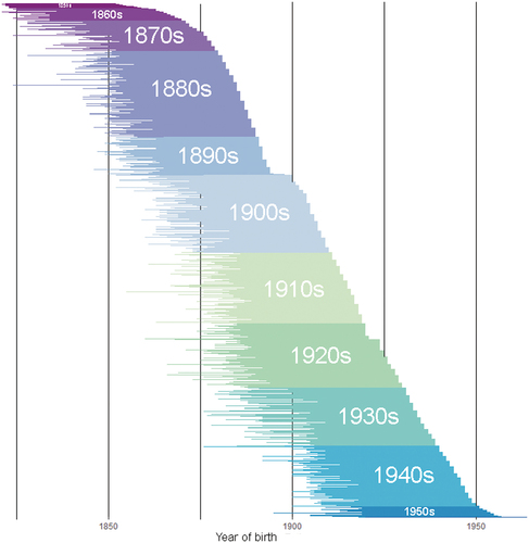
The data on heights are taken from Dutch conscription records that were linked to the Historical Sample of the Netherlands (HSN), a representative sample from Dutch birth records enriched with life course information (HSN, 2010a, 2018). The conscription data do not suffer from large biases (Quanjer & Kok, 2020). The HSN allows for linkages between the HSN research persons (RPs) and their fathers and sons, who were also traced in the conscription records (HSN, 2019). This resulted in a dataset of 3173 father-son linkages, with the HSN RP as either the father or son. This is shown in Figure 1 for sons born between 1850 and 1960. The sample size is limited at the start and end of the research period as linking was restricted by the availability of conscription data. Also, both world wars influenced conscription and therefore appear as a gap in the late 1890s and early 1920s in Figure 1.

Figure 1. Linkage of fathers and sons per year of birth.Note: Each horizontal line represents an observation with a father and a son. The start of the line represents the birth year of the father, the end of the line that of the son. The observations are ordered per birth year of the son along the Y-axis.

2.2. Height data of the research persons

During the research period, Dutch men not only grew taller, but they also reached their adult height earlier (Van Wieringen, 1972). Especially in the middle of the nineteenth century, most men reached their adult height after conscription (Oppers, 1963). Furthermore, from the birth cohort of 1843 onwards, conscripts were measured one year later in life (Koerhuis & van Mulken, 1986), changing the average age of conscription from 18.65 to 19.65. As a consequence of still growing conscripts, the average conscription height for those born in and after 1843 was 2.5 cm higher than that of those born before 1843. The average age of conscription changed again in 1892 and 1902, respectively shifting the average age to 19.32 and 19.52, yet this had a neglectable effect on average height. The same is true for the postwar shift to 18.5 years.

Conscription height is therefore influenced by changing measurement ages as well by the changing growth curve. For a contemporary study, it would also not be feasible to compare the height of the father at age sixteen with the height of the son at age thirteen. It would be impossible to answer if a son outgrows his father as the analysis is clouded by different measurement points at both respective growth curves. Therefore, adult height needs to be estimated to be able to juxtapose both heights and extrapolate the results to other contexts.

The HSN data are limited to only one point of measurement. Nevertheless, a wide range of studies collected Dutch conscription data and linked it to civic guard registers (Beekink & Kok, 2017; Hornix et al., 2020; Kok, 2023; Oppers, 1963; Thompson et al., 2020). In the Netherlands, a civic guard duty was mandatory for all men aged 25 from 1828 to 1908. All men were measured again, which provides an adult height measurement that can be linked to the conscription height. Given the official nature of the civic guard examination, the selection biases into the civic guards are expected to be limited and relatively similar to those of the conscription records. However, not all civic guard registers survived, preventing a linkage with the HSN data. These studies provide us with an insight into growth after conscription at an individual level and will be used to estimate adult heights. Without exception, these prolonged growth trajectories show that shorter individuals at conscription tended to catch up more than taller individuals. This stems from the fact that both short stature and an extended growth trajectory are indicators of deteriorated early life conditions. Therefore, conscription heights themselves are currently the best available indicator of expected growth after conscription.

To estimate the adult heights, generalised additive model smoothing (Hastie & Tibshirani, 2017) was used to fit multi-degree polynomials on the individual level data with conscription heights as the independent and civic guard height as the dependent variable. The extracted formulas were then used to estimate adult heights for the conscription heights in the HSN data. Separate polynomials were used for those born before and after 1843 due to the shift in conscription age. An extensive overview of how the adult height estimate was calculated can be found in appendix 5.1a (including formulas and figures).

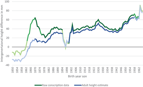
The results of the adult height estimation are plotted together with the raw data in Figure 2. The outcomes in the nineteenth century were particularly influenced by the applied correction. From the start of the secular trend in the 1860s, intergenerational growth appears to be relatively stable until the 1940s for the raw data, but a clearer upward trend is visible for the adult height estimate. In this article, height differences using the adult height estimate will be used as an outcome variable. Still, to test for the robustness of the models, the raw data will be tested as well (see appendix 5.3a).

Figure 2. Raw conscription data and adult height estimate for the height difference between father and son in the Netherlands per birth year (five year moving average) of the son 1850–1965.Note: three color scales are applied to show the number of observations underlying the data. The darkest color line has 50+ observations, the lightest color line has less than 25 observations, the line with the color scales in the middle has between 25-50 observations.

In the analysis of the height difference between father and son, the adult height estimate of the father will also be included as a baseline figure for intergenerational growth. First of all, since it may be harder to outgrow a taller father. Second, the height of the father might have resulted in a more successful life course, which is not reflected in the crude measures used in the analysis. For example, a better earning carpenter would still be in the group of skilled labourers. To reduce multicollinearity with the dependent variable, the height of the father is added as a z-score (the number of standard deviations an observation is located from the group mean) based on the birth cohort of the son.

2.3. Paternal socioeconomic status

One of the most telling characteristics of the paternal life course is socioeconomic status (SES). Both the paternal socioeconomic status and paternal height are to a large extent determined by the socioeconomic status of his own father. The retrieval of the socioeconomic status required various strategies. The HSN database was originally designed for intragenerational research. This means that the life course of the HSN RP is well documented. However, no civil records of either the father or the son of the HSN RP are included in the data. What makes this extra complex is that father-son linkages can be both upward and downward from the perspective of the HSN RP. Figure 3 shows how the socioeconomic status was retrieved in both scenarios. The socioeconomic status the father experienced during his own early youth (I. in the figure) could be accessed through either the paternal occupation stated on his own conscription record or through the paternal occupation stated on his own birth certificate. The socioeconomic status of the father during the early life of his son (II.) was determined through either the paternal occupation on the birth certificate of his son or through the occupation given on his own marriage certificate. All occupations were standardised using the HISCLASS scheme (Mandemakers et al., 2018; Van Leeuwen & Maas, 2011).

Figure 3. The retrieval strategies of occupation of the father’s father (I) and of the father during the early life of the son (II).

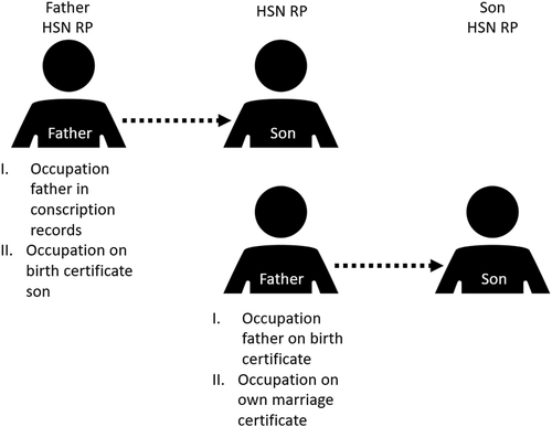
The different strategies in Figure 3 result in occupations being retrieved at different stages of the life course. Therefore, this study is written under the assumption that the HISCLASS category remains constant during the early life of the research person. This is problematic as this will result in an underestimation of the number of socially mobile fathers. Still the groups for which we found a contrast between I. and II. in Figure 3 most likely reflect a true change in socioeconomic class.

The contrast between the socioeconomic status during the early life of the father and that of the son can be used to determine if the father was able to provide his children with a better early life than he experienced himself. If he achieved upward social mobility during his life course, this would translate into a higher probability of his son outgrowing him. This becomes evident from Figure 4, which shows a relatively constant socioeconomic height gap in the Netherlands for the period under study. In line with earlier findings, measuring conscripts one year later reduced this gap, as is visible between the 1840s and 1850s cohorts. What is interesting is that the average gap remains relatively stable over time, despite the changing socioeconomic structure of the economy. During the period under study, manual jobs became more specialised and more white collar workers were needed in the economy (Van Zanden & Van Riel, 2000). Those growing up in an unskilled household amounted to around 40% in 1850, this figure declined to 30% in 1920 and only 10% in 1950. On the other hand, skilled jobs rose from 28% in 1850, to 34% in 1920 and to 36% in 1950, and the middle class amounted to 15, 19 and 35% for these respective years (Rosenbaum-Feldbrügge, 2019; data from this article).

Figure 4. Heights by social class and height differences between (un)skilled workers and others in the Netherlands 1810–1960.Note: No confidence intervals are shown as the differences are not significant due to a low number of observations per cohort. However, the sable nature of the SES difference results in a significant difference for wider cohort spans. The difference between 1840 and 1850 can be ascribed to the change in age at measurement as described in section 2.2. The post-war cohorts suffer from a low number of observations, see figure 1.

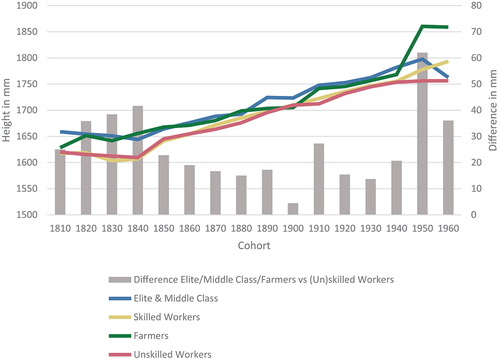
Social mobility can be divided into structural mobility and circular mobility. Those who were ‘forced’ out of their sector as a result of a changing economy are labelled structurally mobile, while those who were promoted on the basis of their achievements are called circularly mobile. The larger the share of circular mobility, the more ‘open’ an economy is. Prior to 1900, the Dutch economy was less open than during the early twentieth century (Delger & Kok, 1998; Van Leeuwen & Maas, 1997). However, for height outcomes, the nature of social mobility seems to have mattered little as a higher social class translated into a taller stature, as is shown in Figure 4. This is why this article does not differentiate between types of mobility and just assesses whether the later-life SES of the father differs from his early-life SES.

Because Figure 4 clearly shows a divide between the elite and middle classes and both skilled and unskilled workers, these last two will be grouped together as a low socioeconomic group. Farmers are included in Figure 4, but will be reviewed as a separate group as there are enormous regional differences in farming that result in a very heterogeneous group in terms of wealth and social status. Therefore, it differs per region if a transition in or out of farming can be viewed as upward or downward mobility, which might cloud the analysis.

Social mobility allows for a comparison between fathers and sons who grew up in different socioeconomic layers of society. Three different analyses will be used. First, an OLS regression will be used with the height difference between father and son as the dependent variable and the socioeconomic class of the father as the dependent variable. It will also be examined what the effect of social mobility of the father on the intergenerational height differences is. Also, for a small subsample (n = 1891), it was possible to extract paternal occupations of the father of the mother through marriage certificates (HSN, 2010b). Hence, it is possible to examine social mobility in the marriage of the father as well.

In the case of upward mobility, was a son taller compared to his father because he grew up in a higher social class than his father? To accomplish this, the son will be juxtaposed to his socioeconomic peers based on a cohort and socioeconomic specific z-score of height. But, his height will also be contrasted against the peers of his own birth cohort, who grew up in the socioeconomic layer of his father (see Figure 5). Two separate analyses using the different z-scores enable us to determine if sons are as tall as their socioeconomic peers or still have the stature of their fathers’ old social layer. The sons of families that did not change socioeconomic class between generations will have two identical z-scores and will be used as the reference category.

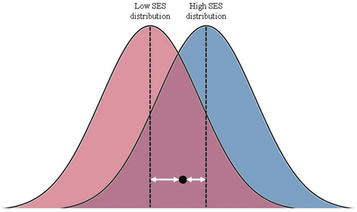
Figure 5. Schematic display of the calculation of both z-scores per cohort and socioeconomic layer in the event of upward mobility.Note: In blue the height distribution of the high SES group of the cohort in which the son grew up (actual situation) and his position relative to the mean (z-score). In red the height distribution of the low SES group of the same birth cohort, but the social layer of his father (hypothetical situation) and again the son’s position relative to the mean.

The rewards of tallness may include social mobility (Thompson et al., 2022). Especially if fathers are relatively tall, this might explain why their sons will even be tall among their new higher socioeconomic peers. Therefore, a similar approach will be used for the heights of the fathers, who are responsible for the social mobility measured in the previous analysis. Again, upward mobility is used as an example. A cohort and socioeconomic specific z-score for height is calculated for the father within the lower group he grew up in. This shows if he was already taller than his peers, which might be rewarded with social mobility. A second cohort and socioeconomic specific z-score for height is calculated for the higher group he moved to. This indicates if he was already as tall as the new group he moved to. This reveals whether the son’s relative height position within his high socioeconomic group is influenced by his father’s height.

Finally, to understand how important class was in the determination of the heights of both father and son, the correlation between their heights is calculated. A lower correlation is expected for earlier cohorts and lower socioeconomic classes (Alter & Oris, 2008). Such a lower correlation would indicate the stronger importance of external factors. The correlations will be compared in a forest plot. In the main article, the models are limited to the contrast between middle classes, skilled workers, and unskilled workers as they comprise the majority of observations. The full models can be found in appendix 5.4a.

2.4. Family composition

Another aspect of the paternal life course that could affect height outcomes is family composition. At the individual level, couples might be influenced by social and religious norms, but their socioeconomic background and height might also play a role. During the period under study, the number of children per couple decreased. This trend began in the upper economic strata and gradually spread to other socioeconomic groups (see appendix 5.5a, Figure A7, Bras et al., 2010; Dribe et al., 2017). Furthermore, a taller father resulted in more surviving offspring and a larger family (Nettle, 2002; Pawlowski et al., 2000; Sear, 2010; Thompson et al., 2021). Paradoxically, a higher number of siblings is associated with a lower height of the offspring due to resource dilution within a family (Hatton, 2017; Mazzoni et al., 2017; Stradford et al., 2017). The number of siblings is not the perfect variable to capture resource dilution as older children might add to household resources (Quanjer & Kok, 2019), but the HSN only allows for a precise reconstruction of RPs’ life courses, not for the fathers or sons. Still, from 1945 on, the conscription records contain information on sibship size and birth order that could be used. This allows for a household reconstruction of two generations, determining if the father grew up in a larger household than his children did. Unfortunately, for fathers of HSN RPs, no household information was available, reducing the analysis to 680 observations and excluding the earlier cohorts from the analyses. Therefore, a smaller sample is used in the analysis of household factors, which will be elaborated on in the descriptive statistics and discussion.

Birth order is also used in the analyses. This might pose an interesting contrast to sibship size as the birth order of a RP is random and not affected by height or the socioeconomic status of the father. Still, both variables do correlate, as in larger families, higher birth orders are possible. To reduce this correlation, the birth order index is used (Booth & Kee, 2009). The variable is constructed as: birth order/((number of children+1)/2) and is already used in the anthropometric literature (Ramon-Muñoz & Ramon-Muñoz, 2017; Öberg, 2015b). In contrast to birth order itself, the birth order index and sibship size can be used in the same model.

2.5. The disease environment

The height difference between father and son is also associated with factors outside the paternal life course. Diseases divert energy from growth, and the difference in disease environments can also contribute to an intergenerational height difference. The disease environment is proxied by the municipal crude death rate per 1000 inhabitants (CDR) between birth and age eighteen (Boonstra, 2016). Recently, Depauw and Oxley (2018) have pointed out that exposure to the disease environment in adolescence captures the effects on heights the best, most likely due to a limited time to catch up. As a result, in this article, the municipal CDR captures the entire early life to reflected more chronic exposure to diseases within a particular municipality. Besides the CDR of that father and the son, maternal CDR conditions are also used based on her place and date of birth.

What might hamper the analysis is the use of CDR to cover a period of more than 150 years. During the nineteenth century, the CDR was mainly driven by infant mortality rates as a result of hygienic conditions, whereas at the end of the research period, after a strong decrease in the CDR, the lifestyles of the elderly drove a large share of the CDR. Still, CDR is the best proxy for the disease environment that stunted the research persons. First of all, the CDR is the longest available annual series at the municipal level, using infant mortality rates would not be feasible because they are only available for multi-year periods. Second, infant mortality rates might not be the best proxy for childhood morbidity, which is why they are often not associated with shorter stature in high mortality contexts (e.g. Stolz et al., 2013; Öberg, 2015a). Childhood mortality may be a better proxy for childhood morbidity, which stunts children. A turning point analysis on a national level found that the decrease in CDR is very similar to that of child and teenage mortality, which started to decline in the 1850s and accelerated in the 1880s, whereas infant mortality only started to decline from 1871 onward (Wolleswinkel-van den Bosch, 1998). Therefore, despite a less steep decline of the CDR, a high CDR is a proxy for high childhood mortality, and a relatively low CDR is a proxy for low childhood mortality.

Furthermore, there is a strong correlation of 0.73 between the CDR of the father’s early life and that of the son. Most likely because the CDR and its developments are heavily affected by region. Especially because the CDR is included for the entire early life, it captures the underlying structural causes of a disease environment and is less likely to be influenced by epidemics. Moreover, a father did have the opportunity to migrate out of an area with a high CDR, but the HSN linkage strategy between father and son reduced the possibility to study long distance migration. Only for HSN research persons who were linked to their sons, migration out of a province did not hamper the linkage. Therefore, the CDR also captures local disease patterns, resulting in the high correlation. To test the robustness of the models, a z-score – the relative position of that municipality in a particular cohort – was used, which might not necessarily be the same for father and son (correlation of 0.25). This did not result in different outcomes.

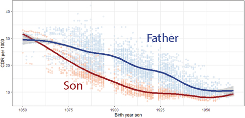
Figure 6 shows the CDR during the early lives of the father and son per birth year of the son. The figure shows that relatively modern CDR standards of below 10 per 1000 were reached in the early 1920s for sons. Yet, their fathers experienced a relatively high CDR during their own childhood. Only when the 1920s generation of sons had children of their own, around 1950, did both father and son experience low CDRs. This coincides with the rise in intergenerational growth shown in Figure 4. This may illustrate a possible intergenerational effect of CDR. Although there are studies that found that even living conditions of earlier generations affected health of later generations (Bygren et al., 2001; Kaati et al., 2007), Kok (2023) found no intergenerational effects on height. To test this, two OLS regressions were run with the intergenerational height difference and the height of the son as outcomes.

Figure 6. The municipal crude death rate per 1000 (left panel) and national caloric availability x 100 (right panel) for father and son per birth year of the son. Data from: HSN (2019) and Boonstra (2016)

The choice for OLS models is motivated by the current nature of the data. It is not feasible to use, for example, a multinominal logistic regression to categorise fathers and sons as tall or short given the dispersed nature of the individual level data over both time and space. With such a method, it would be too complex to identify all biases within the reference groups. Additionally, an OLS is a viable alternative because the majority of the variables are included as dummies. There is no issue with linearity in terms of socioeconomic status, sibship size, or birth order (Quanjer & Kok, 2019). For CDR, it does not affect the main estimate in a problematic fashion. Finally, robust standard errors were employed (Newey & West, 1987; White, 1980) to account for possible problematic heteroskedasticity or correlation inside the models, produced by the stretched nature of the data, which had no impact on the significance outcomes of the models.

3. Results

3.1. Descriptive statistics

Descriptive statistics of the most important variables used in the analysis are reported in Table 1, for the two samples used. As no household information was available for the fathers of HSN RPs, the earlier cohorts were excluded from the analyses on household factors. Therefore, the height figures for the second sample are higher than the first. Furthermore, sons in the first sample had on average more favourable early life conditions than their parents. In the household sample, the household data for father and son are, on average, nearly identical. Running the external factors analysis on the household sample only did not alter the results in a problematic fashion, therefore maximising the number of observations per analysis was chosen as a research strategy. Finally, the height inequality is much higher for the uncorrected heights. This is exactly what is expected with the use of adult heights.

Table 1. Descriptive statistics.

	The full linked father son dataset				Household data (N = 680)
	Avg.	Sd.	Min.	Max.	Avg.	Sd.	Min.	Max.
Height variables
Height Son in cm*	173.5	6.3	156.2	199.5	177.5	6.2	160.4	199.5
Height Father in cm*	170.2	5.5	152.0	191.5	172.9	5.7	156.9	192.0
Difference between son and father*	3.3	6.0	−26.0	27.2	4.5	6.1	−16.2	27.2
Crude death rate in early life
Son	13.7	5.3	6.6	33.1	-	-	-	-
Father	20.9	6.0	8.4	42.2	-	-	-	-
Mother	20.3	6.1	7.8	47.3	-	-	-	-
Household variables
Sibship size son	-	-	-	-	5.4	3.3	1^†	16
Sibship size father	-	-	-	-	5.3	3.5	1	17
Birth order index son	-	-	-	-	3.5	3.3	1	13
Birth order index father	-	-	-	-	3.2	2.2	1	14

Note: *The average height of the son in the unadjusted conscription data is 172.4 cm, with a standard deviation of 7.4 cm. The average height of the father is 168.2 cm with a standard deviation of 7.3 and the average height difference is 4.2 cm with a standard deviation of 7.4. † The sibship size is the total number of children in a household, including the research person.

3.2. Paternal socioeconomic status

Table 2 displays the estimation results of the models with as dependent variable the height difference between father and son and socioeconomic variable as main independent variable. The first model shows that the socioeconomic status of the father during his own early life has no effect on the amount by which his son was able to outgrow him. In other words, the height difference is the same for all socioeconomic groups controlled for birth cohort and region. However, from model 2, we learn that if the height of the father was added as a baseline to grow from, fathers who stem from middle class or farmer households have sons who outgrow them by half a centimetre more than those from an unskilled background. The socioeconomic variable strongly correlates between father and son, as most fathers remained within their social class during their life course. However, model 3 shows what happened to the height difference between father and son if the model included fathers who experienced social mobility during their life course. The overall positive and significant SES association with the height difference increased to one centimetre for the middle class and farmers compared to unskilled workers. Furthermore, fathers who experienced upward social mobility, or mobility into farming created an opportunity for their sons to outgrow them by more. These two groups were significantly associated with a larger height difference between father and son compared to fathers and sons who grew up in the same socioeconomic group. In model 4, the socioeconomic background of the mother during her early life was added, albeit for a smaller sample. A woman who spent her life in a farming household and married a man from a non-farming household was associated with a large height difference between father and son. Interestingly, by adding the SES of the mother, not the positive association of fathers who experienced upward social mobility is significant in model 4, but the negative association of fathers who experienced downward mobility.

Table 2. The association of SES, birth region and birth year and relative height of the father with intergenerational growth, using three methods for growth estimation.

	Adult height estimation
	Model 1	Model 2	Model 3	Model 4
SES father’s early life
Elite	−15.67	−9.61	−5.31	−12.20
Middle class	−0.68	6,20 *	10.12 **	12.70 ***
Skilled workers	−0.59	−0,55	1.52	2.44
Farmers	0.47	7,71 *	10.33 **	12.02 **
Unskilled workers	Ref.	Ref.	Ref.	Ref.
No/Unknown	0.36	3.00	8.49	10.64
SES sons’s early life
Same as son	-	-	Ref.	Ref.
Son higher	-	-	6.69 *	4.57
Father higher	-	-	−4.75	−8.07 ‘
Son farmer (father not)	-	-	11.14 ‘	12.63 ‘
Father farmer (son not)	-	-	1.89	3.56
Unknown	-	-	−3.10	0.74
SES mother’s early life
Same as father	-	-	-	Ref.
Mother higher	-	-	-	5.32
Father higher	-	-	-	−0.45
Mother farmer (father not)	-	-	-	10.63 *
Father farmer (Mother not)	-	-	-	1.07
Unknown	-	-	-	−6.22 *
Z-score father	-	−29.86 ***	−30.12 ***	−30.56 ***
Constant	22.08	22.03	19.39	22.37
R^2	0.032	0.249	0.251	0.261

Note: Significance levels: 0 *** 0.001 ** 0.01 * 0.05 ‘ 0.1. The models uses the adult height estimation and the difference between father’s and son’s height as the dependent variable. The models are controlled for region of birth and birth cohort.

The effect of relative paternal height is negative and substantial. Sons who had a father one standard deviation taller than his peers were less likely to outgrow him. On the other hand, because a z-score was used, sons who had a father who was one standard deviation shorter than his peers were more likely to outgrow him. This is an indicator of regression to the mean, which can be found in most intergenerational studies (see, for example, the very first study by Galton, 1886 and the appendix: section 5.6a).

The models cover a period of more than a hundred years, for which the estimates might be different at different periods. However, the estimates appeared to be relatively stable when an interaction with the birth cohort was tested (results not shown, see appendix 5.2a). Two cohorts appear to have had a significant interaction. In the 1900s cohort, the unskilled workers grow three centimetres more than the other groups. In the 1950s, the middle classes grow five centimetres more than the reference category. Still, the 1950s cohort is limited by the number of observations.

To explore the changes over time more, Figure 7 shows the correlation between the heights of the father and the son. For clarity, only three socioeconomic groups are shown (the full results can be found in the appendix 5.4a). For the early periods, there seems to be somewhat of a social gradient in the correlation coefficients, although the differences are not significant for all groups. Alter and Oris (2008) had similar outcomes for the heights of Belgian brothers. They found that in higher socioeconomic environments, the correlation between brothers’ heights was higher. The cautious conclusion is that paternal inheritance is much smaller in the lower classes, particularly in older cohorts as circumstances were less protective. Environmental conditions claim a larger share in determining height outcomes for these groups.

Figure 7. Correlation coefficients of the estimated adult height of father and son for three socioeconomic groups in five cohorts in the Netherlands.Note: the full figure can be found in the appendix 6.4a.

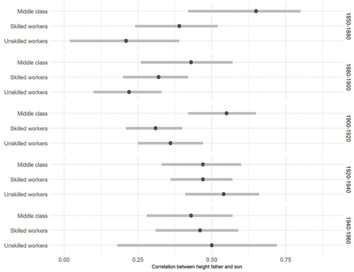
Note: the full figure can be found in the appendix 6.4a.

The social mobility of the father during his life course seems to have been positively associated with the height difference between father and son. This raises the question of whether the son of a father who experienced this social mobility is also taller than his own peers. Does the path dependency of one’s socioeconomic early life determinants matter? This is examined in Table 3. In the first model, the outcome variable is the z-score for the son in the socioeconomic group of his early life (as achieved by his father) and of his own cohort. The sons who grew up in a higher social layer than their father were 0.09 standard deviations shorter than their high-class peers, whose fathers did already belong to the upper class. This association was only found for upward mobility into the middle class or elite, no significant effect was found for a shift into farming. On the other hand, sons of fathers who ascended the social ladder to a lower socioeconomic class were 0.20 standard deviations taller than their lower socioeconomic peers, whose father had already grown up in a lower socioeconomic group. A similar association was also found for farmers.

Table 3. The effect of an intergenerational shift in early life SES between father and son on relative height.

Variable	Early life HISCLASS shift, father → son	Obs.	Son in his SES group & cohort	Son in his cohort & father’s SES	Father in his SES group & cohort	Father in his cohort & Son’s SES
Similar early life HISCLASS	Same class	2085	Ref.	Ref.	Ref.	Ref.
Upward mobility	(Un)skilled workers → Elite & Middle class	367	−0.09 ‘	0.11 *	0.17 **	−0.08
Downward mobility	Elite & Middle class → (Un)skilled workers	130	0.20 *	−0.01	−0.16 ‘	0.06
Downward mobility into farming	Elite & Middle class → Farmers	11	0.62 *	0.38	−0.33	−0.26
Upward mobility into farming	(Un)skilled workers → Farmers	80	0.03	0.17	0.42 ***	0.20 ‘
Downward mobility out of farming	Farmers → (Un)skilled workers	59	0.20 ‘	0.03	−0.05	0.19
Upward mobility out of farming	Farmers → Elite & Middle class	28	0.16	0.25	0.23	0.10
Z-score father in his birth cohort & HISCLASS group			0.40	0.41	-	-
Intercept			0.043	0.046	0.046	0.041
R2			0.1524	0.1572	0.0095	0.0013

Note: The number for this analysis was reduced to 2760 due to the fact that not all socioeconomic backgrounds of fathers could be retraced. Furthermore, if father or son had no/unknown occupation they were excluded from the analysis. Significance levels: 0 *** 0.001 ** 0.01 * 0.05 ‘ 0.1.

In the second model the outcome variable is the z-score for the son in the socioeconomic group that his father grew up in, but of his own birth cohort. This hypothetical situation enables us to determine the effect of different early life conditions as the result of social mobility. Although the first model shows that the sons of fathers who experience upward mobility are still shorter in their new group, the second model shows that these sons are positively (0.11) affected by the newly achieved family context as they are significantly taller than those who remained in the lower classes. The group that experienced downward mobility of the father is associated with a negative effect (−0.01), but this is very small and not significant. Therefore, these sons are presumably not stunted by their lower class environment. They are relatively as tall as the upper class in which their father grew up, which might also explain why they are found to be taller than their peers in the first model. In the second model, no significant effects for farming were found.

The models for the son are controlled for the father’s relative height. Still, to gain a better understanding of the rewards of tallness, the last two models have the relative height of the father as an outcome. The third model shows that those fathers who experience upward mobility are indeed 0.17 standard deviations taller than their peers. The opposite is also found, as those who experience downward mobility are 0.16 standard deviations shorter than their peers. As the father’s stature is significantly different from the group they leave behind, they do not significantly differ from their new socioeconomic group, as is shown in the last model. This shows that their own heights did not provide their sons with a head start in the socioeconomic group they achieved during their life course, although the estimates for upward mobility in the first and last models are strikingly similar. Finally, a strong height bonus of 0.42 standard deviations was found for fathers who moved upward into farming and were taller (0.20) in this group as well.

3.3. Family composition

Table 4 displays how household composition is related to intergenerational growth. The sibship size of the household in which the son grew up is negatively associated with the height difference between father and son, whereas the paternal sibship size had a positive effect. The direction of the effect of the birth order index is positive for both father and son. The effect of the paternal birth order index is only significant in the penultimate model of the table. On the other hand, the son’s birth order index seems to indicate a positive effect of being born last in line on intergenerational height differences.

Table 4. The association of household early life factors of the son, father on intergenerational growth in millimetres, using the adult height estimation.

	Model 1	Model 2	Model 3	Model 4	Model 5	Model 6	Model 7	Model 8	Model 9
Sibship size son	−0.90 *	−1.02	−1.99 **	-	-	-	−0.86 *	−1.46 ‘	−2.28 **
Sibship size father	-	2.97 ***	1.89 **	-	-	-	-	3.03 ***	1.95 **
Birth order index son	-	-	-	10.51 **	19.01 **	10.95 ‘	10.38 **	19.43 **	13.01 *
Birth order index father	-	-	-	-	9.05	4.94	-	11.17 *	6.52
Z-score father	-	-	−31.07 ***	-	-	−30.56 ***	-	-	−30.36 ***
Constant	16.49	−74.67	−53.70	2.25	−91.03	−77.29	7.83	−112.54	−79.16
R^2	0.031	0.039	0.239	0.034	0.033	0.229	0.036	0.054	0.242

Note: Significance levels: 0 *** 0.001 ** 0.01 * 0.05 ‘ 0.1, all models are controlled for SES, birth region and birth cohort. The adult height estimation is used for the difference in height between father and son, which is used as the dependent variable.

Whereas in Table 4, the height difference between the father and the son is used as the outcome variable and is compared with other father-son pairs. Table 5 uses the relative height of the son and compares it with his peers. This is done because, from Table 4, it is unclear if the variation in height differences between father and son stems from the effects on the height of the father or from effects on the height of the son. By studying the height of the son, it becomes clear if the effect of the sibship size of the household in which the father grew up also had an effect on the height of the son. What stands out from Table 6 is that only the sibship size of the son has a negative effect on his relative height. The sibship size of the father results in a small and non-significant effect. Furthermore, the birth order index has no effect on the relative height. This is surprising, as other studies (e.g. Quanjer & Kok, 2019) have found a positive effect of birth order, similar to that in Table 4. The difference might be the result of using different birth cohorts. Also, the limited number of fathers with household information might have been a limiting factor, which might also have altered the results.

Table 5. The association of household early life factors of the son, on relative height of the son (z-score).

	Model 1	Model 2	Model 3	Model 4	Model 5	Model 6	Model 7	Model 8	Model 9
Sibship size son	−0.04 ***	−0.05 ***	−0.03 **	-	-	-	−0.04 ***	−0.05 ***	−0.03 **
Sibship size father	-	0.00	0.02	-	-	-	-	0.00	0.02
Birth order index son	-	-	-	0.00	−0.12	0.00	−0.00	−0.04	0.04
Birth order index father	-	-	-	-	0.06	0.11	-	0.06	0.13
Z-score father	-	-	0.43 ***	-	-	0.44 ***	-	-	0.43 ***
Constant	0.21	0.40	0.21	0.01	0.22	0.01	0.22	0.38	0.05
R^2	0.035	0.056	0.209	0.020	0.040	0.202	0.035	0.055	0.210

Note: Significance levels: 0 *** 0.001 ** 0.01 * 0.05 ‘ 0.1, all models are controlled for SES, birth region and birth cohort. The dependent variable is the relative height of the son, within his birth cohort.

Table 6. The association of crude death rate (CDR) during the early life of the son, father and mother on the intergenerational height difference in millimetre, using the adult height estimation.

	Model 1	Model 2	Model 3
Crude death rate
CDR son’s early life	−1.81 **	−2.49 ***	−1.89 ***
CDR father’s early life	-	1.59 ***	0.85 **
Mother experienced same CDR as father	Ref.	Ref.	Ref.
Mother experienced lower CDR than father	-	−4.13	−3.91
Mother experienced higher CDR than father	-	−12.05 ***	−8.35 **
Z-score father	-	-	−28.91 ***
Constant	59.84	37.34	41.21
R^2	0.036	0.052	0.250

Note: Significance levels: 0 *** 0.001 ** 0.01 * 0.05 ‘ 0.1, all models are controlled for SES, birth region and birth cohort. The adult height estimation is used for the difference in height between father and son, which is used as the dependent variable.

3.4. The disease environment

Table 6 presents the estimation results of the models that examine the association between the CDR as a proxy for the disease environment and the height difference between father and son. First, the son’s own living conditions were included, followed by the CDRs that his parents experienced during their early lives. Finally, the paternal height is controlled for. The effect of CDR during the early life of the son negatively associated with the height difference with his father. In models 2 and 3, a higher CDR in early life for the father is associated with a larger height difference, even when the relative height of the father is used as a control (model 3). Furthermore, mothers who experienced a higher CDR than the father were associated with a smaller height difference between father and son. However, the reverse result was not found for mothers who experienced a lower CDR.

Table 7 has the same layout as Table 6, but now the outcome variable is the relative height of the son measured as a cohort specific z-score. Whereas the previous table studied the effect of growth compared with the previous generation, Table 4 studies growth differences within a generation. Here we see that the CDR of the son has a negative effect on the relative height of the son, but that the CDR of the father has a negative effect as well. In the third model, this negative effect is captured by the height of the father. Furthermore, we find that the mothers’ CDR is again a restricting factor. Finally, the z-score of the father’s effect of 0.41 points towards regression to the mean, as a father who is 1 standard deviation taller than his average peer will have a son who is still taller than average, but is only 0.41 standard deviation taller than his average peer (see appendix 5.4a).

Table 7. The association of crude death rate (CDR) during the early life of the son, father and mother on relative height of the son in millimetres, using the adult height estimation.

	Model 1	Model 2	Model 3
Crude death rate
CDR son’s early life	−0.03 **	−0.03 *	−0.04 ***
CDR father’s early life	-	−0.01 *	−0.00
Mother experienced same CDR as father	Ref.	Ref.	Ref.
Mother experienced lower CDR than father	-	−0.05	−0.05
Mother experienced higher CDR than father	-	−0.11 ‘	−0.16 **
Z-score father	-	-	0.41 ***
Constant	0.58	0,87	0.82
R^2	0.030	0.032	0.176

Note: Significance levels: 0 *** 0.001 ** 0.01 * 0.05 ‘ 0.1, all models are controlled for SES, birth region and birth cohort. The dependent variable is the relative height of the son, within his birth cohort.

4. Discussion

The main aim of this article was to study how the paternal life course affects height differences between father and son. This is a novel approach, as height differences are often studied within a cohort rather than between generations. To gain a better understanding of intergenerational height differences, external and household factors during the early lives of two generations were examined. Two variables, socioeconomic class and number of children, could be actively influenced by the father during his life course. The two other variables, birth order and disease environment, were related to the paternal life course to a lesser extent. In order to examine if early life conditions had a generational or intergenerational effect, separate analyses were conducted using the height difference between father and son and the relative height of the son as outcome variables.

4.1. Paternal socioeconomic status

The various models used in this study have provided new insights on the association between socioeconomic status and height, and especially the development of height over time. Like earlier studies (Jaadla et al., 2020; Quanjer & Kok, 2019), this study found clear height differences associated with different socioeconomic classes experienced during early life. However, the models on the height difference between father and son, found no clear difference when the height of the father was not taken into account. This could imply that the upward trend in heights occurred at the same rate for all social classes in the Netherlands. Nevertheless, when the height of the father was controlled for, it was found that sons of fathers with a middle class background or a background in farming outgrew him by more than sons with other backgrounds. The association between paternal height and the height difference with his son was negative, which means that it was harder to outgrow a taller father. Because higher SES groups are taller, this suppressing effect of paternal height is hidden in the SES variable, and hence no significant effect was found in the first place.

When a father experienced social mobility in his life course, this affected the height difference with his son in the expected direction. What is more interesting is that when a mother from a farming background married a non-farming man, their son outgrew his father by more than sons from non-farming couples. The exact pathway is unclear, but it may be the result of a taller mother because of her own early life conditions. It may also be the result of better knowledge of food, which translates into a son who is better fed, or simply because of a healthier mother.

Through social mobility, the father not only enabled his son to outgrow him but also to be significantly taller than the son’s lower class peers. Still, the son was not able to fully catch up with his higher class peers. This may help to explain why, even after controlling for the father’s height, there is still a tendency for sons from middle-class and farming backgrounds to have larger height differences with their father than other SES groups.

Finally, it was found that the height of the father was less of a predictor for the height of the son in lower classes than in earlier cohorts. This low correlation is an indicator that the effects of external factors played a larger role for these groups in determining the heights of father and son. This is why the disease environment was also included in this study.

4.2. The disease environment

With regard to the external factors, CDR in the early life of the son had a negative influence on his relative height. Also, the intergenerational height difference was negatively affected by a high CDR of the son. The effect of the CDR of the father was positively associated with their height difference, even when the relative height of the father was included as a control. Still, no effect of the CDR the father experienced was found on the relative height of the son. Therefore, the effect of CDR does not supersede a generation. Still, we can conclude that an improvement in CDR makes a son taller than his father. Furthermore, a mother growing up in a municipality and cohort with a higher CDR than the father can restrict the possible growth of the son. It might very well be that these mothers were restricted in their growth and therefore restricted the growth of the son in utero (Cole, 2003). However, these mothers might also have been scarred in other ways that affected their son’s height, for example, because they had a lower chance of dying during their son’s childhood, which also causes a shorter stature (Quanjer & Kok, 2021).

As mentioned earlier, it does not matter for the outcomes if CDR was included in the analysis as an absolute value, in which the differences are strongly driven by change over time, or as a relative cohort specific z-score, in which the differences are more regional. It can therefore be concluded that a healthier environment results in a taller stature as less energy is diverted from growth. This health effect is limited to one generation, as the effect on the son was positive, that on the father was negative, and there was no effect of the CDR in the early life of the father on the height of the son.

4.3. Family composition

The effect of sibship size operates similarly to CDR. A high number of siblings has a negative effect on the relative height of the son through resource dilution. The number of siblings a father had did not influence the sons’ height, as sibship size influences height within a generation. Consequently, we again find the mirror image in effects for father and son when the difference in their heights is used as the dependent variable. A father who was raised in a large sibship was associated with a shorter stature, and his son was more likely to outgrow him. If a father had many children himself, he reduced the opportunity for his son to outgrow him.

Birth order of the son has a positive and significant effect on growth, whereas the birth order of the father seems to have no effect. The early life conditions of the youngest child seem to have been more favourable to outgrow their fathers. This height of the sons is also positively affected, although not significantly.

4.4. The effect of the paternal life course on the secular trend

This novel approach has shown that fathers were indeed able to provide their offspring with better early life conditions, and as a result, their offspring was able to outgrow them. However, these results are intertwined in a complex mechanism of rewards and consequences of tallness. Tallness is rewarded on the marriage market (Thompson et al., 2021) and increases the survival rates of offspring (Sear et al., 2004). Therefore, taller men might have larger families, which reduces the height of their offspring. Nevertheless, in line with the demographic transition theory, increased survival rates are an incentive to limit the number of offspring. Furthermore, higher SES families, who are on average taller, tended to have fewer children (Dribe et al., 2017; Öberg, 2017). Also, the benefits of tallness are not linear, and therefore, extreme tallness might have a negative effect on the paternal life course. It is beyond the scope of this study to determine how a successful paternal life course resulted in a taller population as a whole on the one hand while also keeping height inequality in check because of the unsuccessfulness of an extremely tall stature and because a tall stature resulted in more offspring on the other.

4.5. Limitations

There are two data issues that need to be discussed as they might have affected the outcomes. The first is the construction of the dataset. All HSN RPs were taken as a starting point. Some of these RPs were linked to their father and are therefore taken from a representative sample, as all sons have a father that could be searched for. On the other hand, the HSN RPs who take on the role of father are linked to one of their sons and are selected on the condition that they have at least one son. It has been shown that taller men have more surviving children (Thompson et al., 2021), so there might be a height bias for this group. This assumption was proven by a logistic regression on the data, the RPs that were successfully linked to their father were slightly taller (Odds ratio of 1.03 for cohort based z-score), but the difference was not significant (p = 0.43). On the other hand, RPs that were successfully linked to a son were also taller (Odds ratio of 1.10 for cohort based z-score) and the effect was significant (p = 0.01). Furthermore, by adding height as a quadratic term, the odds of the linear effect remained unchanged, and the quadratic term resulted in a significant parabolic relationship (odds are 0.93, p = 0.01). To address this issue, both analyses were run separately. This did not alter the results in a problematic fashion.

Secondly, the growth estimation might be off in estimating adult height. Still, this did not change the results drastically, so the overall story of the paper remains the same. The strongest change is found in the early period. The correlation between the heights of father and son changed from 0.35 to 0.38 in the period prior to 1880, when the adult height estimate was used. The change is small, and also exactly what can be expected, as adult heights are more likely to correlate than height somewhere along the growth curve. For the later periods, conscription heights reflect adult heights better, and the change in correlations is even less.

The use of a growth estimate for the historical population is especially useful when individuals are studied. Especially for shorter individuals, extreme catch up growth might alter results. Nevertheless, the proposed estimation formulas are only based on Dutch data. Still, this would not imply they are limited to solely a Dutch context, but evidence is absent that they would fit universally into all human frameworks. The most important point is the awareness that within population variation can be strongly influenced by differences in growth trajectories due to the moment of measurement.

4.6. Conclusion

By using an intergenerational perspective on height differences, this study provided new insight on the development of heights over time. Despite clear socioeconomic height differences, the difference between father and son remained very stable within the Netherlands. Only when paternal height was controlled for did differences become apparent. The father, through his life course, could also affect the height difference with his son through social mobility. His son could then have benefitted from the circumstances in a higher socioeconomic layer, although he could not directly catch up with his high class peers. Social mobility through marriage also affected the height difference, but this could also be related to the early life conditions of the mother herself. A higher CDR also reduced the possibility for a son to outgrow his father. The main conclusion is that both household factors and external conditions affect the height of the particular generation growing up in them. These conditions can change between lives, and as a result, the Dutch were able to grow taller during the period under study.

What this study showed is that we should be aware that a factor such a socioeconomic status which is added as a constant variable in a model can be path dependent. Social mobility can affect heights of successive generations compared to families that remained within their class. This study also pointed out that we should be aware of the role of the mother, especially how her early life conditions affected the heights of her offspring. As digital linking will result in more complex and extensive datasets in the future, we will be able to incorporate such dynamics in more studies and use a more dynamic intergenerational approach compared to the static intragenerational studies. This study has shown that such an approach can yield insights on to how extraordinary life courses can affect multiple generations in history.

Disclosure statement

No potential conflict of interest was reported by the author.

Additional information

Funding

This research is funded by the Netherlands Organisation for Scientific Research (NWO), Giants of the modern world project, 360-53-190.

Notes

1. Based on the data of the current article.

Appendix

5.1a Constructing an adult height estimate

A wide range of studies has shown that Dutch conscription height is not the same as terminal adult stature, especially in the nineteenth century (Kok, 2022; Oppers, 1963; Thompson et al., 2020). This poses no problem for a study into living standards, as differences in early life conditions are more pronounced in conscription heights (Beekink & Kok, 2017; Hornix et al., 2020). However, it is problematic to compare heights across generations. A son might have reached his final height at conscription, whereas his father still grew at his own conscription measurement. To place this in context, in modern times this would equal comparing the height of a fifteen to a seventeen year old boy. A problem that could be fixed by using height-for-age z-scores (e.g. Schneider, 2020.), but there is no growth reference available for differences in growth after age twenty. Therefore, this appendix will explain how the current article handled the prolonged growth that occurred after conscription.

Most studies, if they correct for growth, add a fixed number of centimetres based on the age of the conscripts. For example, the large database CLIO-INFRA uses Baten and Blum’s (2012) correction based on Mackeprang (1923) adding 2,4 cm to the heights of 18 year olds, 1,7 cm for age 19, 0,9 for age 20, 0,4 for age 21 and 0,1 for age 22. Furthermore, these corrections are only made if the mean is below 170 cm. While these corrections might work well for aggregated data samples, individual level data requires a different treatment. This becomes apparent in Figure A1, which combines all the currently available prolonged growth data for the Netherlands Beekink and Kok (2017); Hornix et al. (2020); Oppers (1963); Thompson et al. (2020); Kok (2022). Growth rates after conscription at the lower end of the height spectrum tended to be much higher than those who were already tall at conscription.

Figure A1: The association between conscription height and adult height in the Netherlands in the nineteenth century.Sources: Beekink & Kok, 2017; Hornix, Kalsbeek, & Quanjer, 2020; Oppers, 1963; Thompson, Quanjer, & Murkens, 2020, Kok, this issue

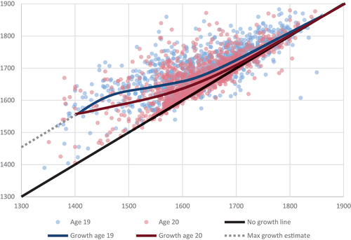
So, what is shown in Figure A1? Placed on the X-axis is the height measured at conscription. However, since the age at which men were subject to conscription was changed from 19 to 20 in 1862, the different colours show these different subgroups in the data. On the Y-axis, the height that was reached by the same individual is shown, now measured at age 25, when he was subject to service in his local civic guard. Generalized additive model smoothing in the geom_smooth command from the ggplot2 package in R was used to estimate the average prolonged growth based on the conscription height. This resulted in the formulas that are used to estimate adult height in this paper:

Based on conscription height (x) measured in the year the conscripted turned 19 (birth year<1843):

$Adult\hspace{0.17em}height=-0,0000000073x^4+\hspace{0.17em}0,0000475x^3-\hspace{0.17em}0,115x^2+\hspace{0.17em}122,21x\hspace{0.17em}-\hspace{0.17em}47089,42$

Based on conscription height (x) measured in the year the conscripted turned 20 (birth year>1842):

$\begin{array}{rl}& Adult\hspace{0.17em}height\hspace{0.17em}=0,00000000000027x^6-\hspace{0.17em}0,00000000254x^5+\hspace{0.17em}0,00001x^4-\hspace{0.17em}0,021x^3+\\ & 24,95x^2-15543,20x\hspace{0.17em}+\hspace{0.17em}4006510,51\end{array}$

The prolonged growth estimate line at age 19 in Figure A1 seems to reach a plafond of fifteen centimetres of additional growth after conscription. It is not unlikely that some individuals grow even more, but at these short heights, growth disorders will likely also influence the final outcomes. Therefore, a rough estimate was used for heights below a conscription height of 1400 millimetres, adding fifteen centimetres for these research persons. In the dataset used for this paper, this affects two RPs.

Over time, the Dutch have been found to grow taller and reach their adult height at younger ages (Van Wieringen, 1972). These changes are driven by underlying living conditions, of which height itself is an outcome. Therefore, the method used is based on the assumption that at taller conscription statures, there is less growth to be expected after conscription since these taller statures were reflective of better living conditions. In doing so, this is our best shot at capturing the differences in growth over time as well as within a particular cohort.

Still, the estimated growth after conscription clearly does not capture the complex variation in the data underneath and is therefore not flawless. It requires a leap of faith from the reader to consent with this method, yet for the historical Dutch data, it is currently the closest estimate available. However, there are indications that the estimations used reflect growth after conscription correctly.

The CLIO-INFRA data only corrects for extra growth below a height of 170 cm. The estimated growth used in this article, after conscription at age twenty, tends to reflects this same threshold. Furthermore, the growth estimates enable us to determine which share of intergenerational growth between father and son might be the result of extra growth after conscription. This is visualised in Figure A2, which shows that in the middle of the nineteenth century, a large share of the height difference between father and son can be attributed to a shift in growth trajectories. This figure can be compared with Figure A3. Figure A3 compares conscripts born early in the year, with conscripts born late in the year. Because a cohort of conscripts was measured over a small interval of a few days, those born earlier were taller because they were older at the time of measurement. This enables us to determine if conscripts were still growing in the year they were measured. The lines in both figures show more or less the same trends, which is encouraging for the adult height estimates. Nonetheless, interpreting both figures is hampered due to the different meaning of the X-axis. In Figure A2, the birth year of the son is shown, yet all these sons are linked to fathers with different birth years to calculate their height differences. In Figure A3, the year of measurement is shown on the X-axis. This is done because the downward trend in Figure A2 coincides with more condensed growth curves for fathers. As the year of measurement of the father is closest to the birth year of the son, this allows for the best visual comparison between both figures. The lines in Figure A3 are not driven by seasonal effects, as a comparison between boys born in January and December yielded the same results but was harder to interpret because of the lower number of observations.

Figure A2: The share of intergenerational growth which is the result of the shift in timing of growth using the adult height estimate and the conscription height estimate from figure 3.

Figure A3: Difference in heights between conscripts born in the first three months of the year compared to those born in the last three months of the year in millimetre 1839–1983.

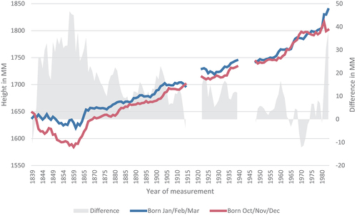
The method used for the article reduces height inequality within the data. This has to do with the fact that more growth is added at the lower end of the distribution. Again, this is echoed by other Dutch data on adolescent growth in the Netherlands in the nineteenth century in undefined A1. The table shows the growth of pupils of the maritime institute in Amsterdam between their entry age in the institute and to their conscription records (Quanjer & Kok, 2021). The data also show higher growth rates for the shorter statures. Furthermore, a maximum amount of growth seems to be determined at the lower statures as well. Both characteristics provide some support for the adult height estimations used in this paper. Still the data of these students in undefined A1 reflects a higher social strata than the conscription records. Therefore, the amount of growth and timing might differ, but the overall pattern will remain the same.

The difference between the two estimates in Figure A1 is used to calculate the growth between the conscripts measured at age 19 and those at age 20. The following formula is used based on conscription height.

$\begin{array}{rl}& Adult\hspace{0.17em}height\hspace{0.17em}=0,00000000000027x^6-\hspace{0.17em}0,00000000254x^5+\hspace{0.17em}0,00001x^4-\hspace{0.17em}0,021x^3+\\ & 25,07x^2-15665,41x\hspace{0.17em}+\hspace{0.17em}4053599,9\hspace{0.17em}+\hspace{0.17em}x\end{array}$

Table A1. Growth of pupils of the maritime institute of Amsterdam 1860–1940 until the conscription measurement.

	Age of measurement
Height in cm	14	15	16	17
135–140	16,9	-	-	-
140–145	20,4	19,7	-	-
145–150	20,6	19,0	-	-
150–155	17,6	15,7	14,5	-
155–160	14,7	12,7	-	7,7
160–165	13,3	8,4	8,6	4,9
165–170	11,1	6,1	5,7	2,4
170–175	6,8	5,4	5,2	2,4
175–180	-	6,1	4,1	1,7
180–185	-	-	3,6	2,5
185–190	-	-	0,0	1,6

Note : Source: Quanjer and Kok (2021).

5.2a Growth of the different SES groups

Below, the development of intergenerational growth is shown for different socioeconomic groups within Dutch society, using the adult height estimate. The socioeconomic groups are grouped together, as was done for the social mobility analysis. Remarkable during much of the period the group show a similar trajectory. The difference before 1860 is striking, as the lower classes experienced less shrinkage. On the other hand, they were already shorter, which might also have reduced the intergenerational shrinkage. These effects were not significantly different in a regression. The gap around 1900 proved to be significant in a regression. This is not the case for the difference in the late 1920s. This might be related to more variance in intergenerational growth within these groups. The gap around 1950 in favour of the higher classes was on the other hand significant again. Still this figure A4 does not signal a rise in inequality over time, or an increasing height gap that was caught up on.

Figure A4: Intergenerational growth per socioeconomic group in the Netherlands per birth year of the son (10 year moving average).

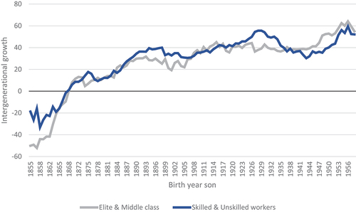
5.3a Robustness of the estimates

This study computes the variables in many ways to deal with, for example, multicollinearity or the growth after conscription. The analysis most prone to the effect of such alterations is the model on CDRs, because there is a high correlation in both the CDR and the height of the father and son. The various ways in which the variables could have been included in the models are presented in undefined A2. The finding that CDR has an effect on height within a generation and therefore stunts a son, and as a result reduced the height difference between father and son, holds in all models. Furthermore, the effect of the mother is also very constant in all models. What is clear is that the estimates for the raw data are slightly higher, which is to be expected as growth after conscription is not included which usually reduces inequality. Furthermore, the strongest variability is found in the estimate of the CDR of the father. This estimate is strongly associated with paternal height as well. As a result, depending on the input of paternal height (either as a z-score or as height in millimetre), the association with the dependent variable is significant or not. The direction of the estimate remains positive for all models. In sum, the various ways in which the variables can be added to the models do not result in different outcomes for this study. Underlying that the main results are robust (See Figure A5).

Table A2. The association of CDR of the son, father, and mother on intergenerational growth in millimetres, using the adult height estimation and the raw data.

	Used model (CDR & z-score height father)	Alternative model 1 (Z-score CDR & z-score height father)	Alternative model 2 (Z-score CDR & height father)	Alternative model 3 (CDR & height father)	Alternative model 4 (Raw data, same set up as first model)
CDR son	−1.89 ***	−4.74 **	−4.95 ***	−1.93 ***	−1.98 **
CDR father	0.85 **	0.84 **	0.31	0.31	1.02 **
Mother has same CDR as father	Ref.	Ref.	Ref.	Ref.	Ref.
Mother has lower CDR	−3.91	−3.76	−3.57	−3.71	−4.77
Mother has higher CDR	−8.35 **	−8.33 **	−8.60 ***	−8.64 **	−10.19 **
Height father	−28.91 ***	−28.95 ***	−0.55 ***	−0.55 ***	−42.45 ***
Constant	41.21	3.81	946.03	982.38	53.76
R^2	0.250	0.252	0.262	0.261	0.312

Note: Significance codes: 0 *** 0.001 ** 0.01 * 0.05 ‘ 0.1., all models are controlled for SES, birth region and birth cohort.

5.4 Full correlation plot

In the main text, the correlation plot was limited to the main variables only. In Figure A6, the full models are shown for all SES groups and for the uncorrected conscription height and for the adult height estimations. The difference between the two is only clear for the earlier cohorts. The correlation for the adult height is higher, as is to be expected. Conscription height also encompasses growth, which is much more influenced by the external environment than by inherited genes.

Figure A5: The number of children in the household of HSN RPs per socioeconomic group between 1860 and 1960.

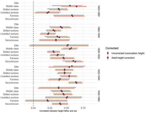
Figure A6: Correlation coefficients of the estimated adult height of father and son for three socioeconomic groups in five cohorts in the Netherlands.

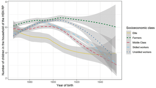
5.5 Sibship size per SES over time

This paper has presented a complex mechanism in which taller men are able to be more socially mobile. As a result of the social mobility, their offspring is taller as well. On the other hand, taller men tend to have more surviving children. A larger sibship size is associated with a shorter stature. What makes it extra complex is that over time, the perverted number of children for couples decreased for different socioeconomic classes at different times. Figure A7 shows the size of the household in which the RPs grew up. This places the complexed interplay between height, SES and sibship size into the context of the demographic transition in the Netherlands.

Figure A7: Illustration of regression to the mean using height of the father (x-axis) and height of the son (y-axis).

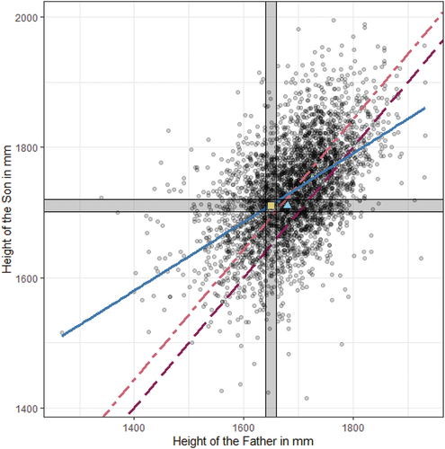
5.6 Regression to the mean

This phenomenon was first described by Francis Galton in 1877, who tried to use his quincunx to understand the intergenerational heritability of height (Pearl & Mackenzie, 2018). Taller fathers will have a taller son, yet this son will be closer (shorter) to the average height of his generation. Paradoxically, taller sons, will have a tall father, yet this father will be closer (shorter) to the average height of his generations. And although both statements seem to contradict each other, both are true. The figure (based on Pearl & Mackenzie, p82.) below shows how this works in the data. Since regression to the mean was found for all growth estimations, the raw conscription data was used in this example, as this demonstrated the mechanism most clearly due to an overestimation of growth.

The dark purple line shows X=Y but due to the secular trend in heights, sons tend to be, on average, taller than their fathers. So the centre line of the ellipse (in red) is X=Y + 4,2 cm which is the average growth between father and son. However, this is not the regression line of the underlying data because of regression to the mean. The regression line is shown in blue. To show what this implies, a column is shown for fathers who are 165 cm tall (between 164 and 166 cm), and the sons in this column are on average 171 cm tall (yellow square). On the other hand, sons who are on average 171 cm (horizontal column between 170 and 172 cm) have on average a father of 168 cm (blue triangle).

References

- Alberman, E., Filakti, H., Williams, S., Evans, S. J. W., & Emanuel, I. (1991). Early influences on the secular change in adult height between the parents and children of the 1958 birth cohort. Annals of Human Biology, 18(2), 127–136. https://doi.org/10.1080/03014469100001472
- Alter, G., Neven, M., & Oris, M. (2004). Height, wealth and longevity in XIXth century east Belgium. Annales de démographie historique, 108(2), 19–37. https://doi.org/10.3917/adh.108.0019
- Alter, G., & Oris, M. (2008). Effects of inheritance and environment on the heights of brothers in nineteenth-century Belgium. Human Nature, 19(1), 44–55. https://doi.org/10.1007/s12110-008-9029-1
- Bailey, R. E., Hatton, T. J., & Inwood, K. (2016). Health, height, and the household at the turn of the twentieth century. The Economic History Review, 69(1), 35–53. https://doi.org/10.1111/ehr.12099
- Baten, J. (2009). Protein supply and nutritional status in nineteenth century Bavaria, Prussia and France. Economics & Human Biology, 7(2), 165–180. https://doi.org/10.1016/j.ehb.2009.02.001
- Baten, J., & Blum, M. (2012). Growing tall but unequal: New findings and new background evidence on anthropometric welfare in 156 countries, 1810–1989. Economic History of Developing Regions, 27(sup1), S66–85. https://doi.org/10.1080/20780389.2012.657489
- Beekink, E., & Kok, J. (2017). Temporary and lasting effects of childhood deprivation on male stature. Late adolescent stature and catch-up growth in Woerden (The Netherlands) in the first half of the nineteenth century. The History of the Family, 22(2–3), 196–213. https://doi.org/10.1080/1081602X.2016.1212722
- Boonstra, O. (2016). Historische Database Nederlandse Gemeenten. IISH Data Collection, V2. https://hdl.handle.net/10622/RPBVK4
- Booth, A. L., & Kee, H. J. (2009). Birth order matters: The effect of family size and birth order on educational attainment. Journal of Population Economics, 22(2), 367–397. https://doi.org/10.1007/s00148-007-0181-4
- Bras, H., Kok, J., & Mandemakers, K. (2010). Sibship size and status attainment across contexts: Evidence from the Netherlands, 1840-1925. Demographic Research, 23, 73–104. https://doi.org/10.4054/DemRes.2010.23.4
- Bygren, L. O., Kaati, G., & Edvinsson, S. (2001). Longevity determined by paternal ancestors’ nutrition during their slow growth period. Acta Biotheoretica, 49(1), 53–59. https://doi.org/10.1023/A:1010241825519
- Case, A., & Paxson, C. (2008). Stature and status: Height, ability, and labor market outcomes. The Journal of Political Economy, 116(3), 499–532. https://doi.org/10.1086/589524
- Cole, T. J. (2003). The secular trend in human physical growth: A biological view. Economics & Human Biology, 1(2), 161–168. https://doi.org/10.1016/S1570-677X(02)00033-3
- Costa, D. L. (2004). The measure of man and older age mortality: Evidence from the Gould sample. The Journal of Economic History, 64(1), 1–23. https://doi.org/10.1017/S002205070400258X
- Deaton, A. (2013). The great escape: Health, wealth, and the origins of inequality. Princeton University Press.
- Delger, H., & Kok, J. (1998). Bridegrooms and biases: A critical look at the study of intergenerational mobility on the basis of marriage certificates. Historical Methods: A Journal of Quantitative and Interdisciplinary History, 31(3), 113–121. https://doi.org/10.1080/01615449809601194
- Depauw, E., & Oxley, D. (2018). Toddlers, teenagers, and terminal heights: The importance of puberty for male adult stature, Flanders, 1800–76. The Economic History Review, 72(3), 925–952. https://doi.org/10.1111/ehr.12745
- Dribe, M., Breschi, M., Gagnon, A., Gauvreau, D., Hanson, H. A., Maloney, T. N., Mazzoni, S., Molitoris, J., Pozzi, L., Smith, K. R., & Vézina, H. (2017). Socio-economic status and fertility decline: Insights from historical transitions in Europe and North America. Population Studies, 71(1), 3–21. https://doi.org/10.1080/00324728.2016.1253857
- Finaret, A. B., & Masters, W. A. (2020). Can shorter mothers have taller children? Nutritional mobility, health equity and the intergenerational transmission of relative height. Economics & Human Biology, 39, 100928. https://doi.org/10.1016/j.ehb.2020.100928
- Galton, F. (1886). Regression towards mediocrity in hereditary stature. The Journal of the Anthropological Institute of Great Britain and Ireland, 15, 246–263. https://doi.org/10.2307/2841583
- Grasgruber, P., & Hrazdíra, E. (2020). Nutritional and socio-economic predictors of adult height in 152 world populations. Economics & Human Biology, 37, 100848. https://doi.org/10.1016/j.ehb.2020.100848
- Groote, P., & Tassenaar, V. (2020). Living standards in a dairy region, 1850–1900: From urban penalty to urban premium. Journal of Historical Geography, 70, 12–23. https://doi.org/10.1016/j.jhg.2020.08.001
- Hastie, T. J., & Tibshirani, R. J. (2017). Generalized additive models. Routledge.
- Hatton, T. J. (2011). Infant mortality and the health of survivors: Britain, 1910–50. The Economic History Review, 64(3), 951–972. https://doi.org/10.1111/j.1468-0289.2010.00572.x
- Hatton, T. J. (2017). Stature and sibship: Historical evidence. The History of the Family, 22(2–3), 175–195. https://doi.org/10.1080/1081602X.2016.1143856
- Hatton, T. J., & Bray, B. E. (2010). Long run trends in the heights of European men, 19th–20th centuries. Economics & Human Biology, 8(3), 405–413. https://doi.org/10.1016/j.ehb.2010.03.001
- Hatton, T. J., & Martin, R. M. (2010). Fertility decline and the heights of children in Britain, 1886–1938. Explorations in Economic History, 47(4), 505–519. https://doi.org/10.1016/j.eeh.2010.05.003
- Hornix, J., Kalsbeek, T., & Quanjer, B. (2020). Lengtegroei, lotelingen en Limburg. Doorgroei van Limburgse plattelandsjongens in Eijsden en Arcen-Velden, 1863-1898. Studies over de Sociaal-Economische Geschiedenis van Limburg, 64, 40–69. https://doi.org/10.58484/ssegl.v64i12329
- HSN. (2010a). Historical Sample of the Netherlands (HSN): Data set civil certificates release 2010.01 [Data file and code book].
- HSN. (2010b).Historical Sample of the Netherlands (HSN): Data set life courses release 2010.01 [Data file and code book].
- HSN. (2018). Historical Sample of the Netherlands (HSN): Data set heights and life courses release 2018_02 [Data file and code book].
- HSN. (2019). Historical Sample of the Netherlands (HSN), Male Kin Height database (MKH): Data set heights and life courses release 2019_05 [Data file and code book].
- Jaadla, H., Shaw-Taylor, L., & Davenport, R. (2020). Height and health in late eighteenth-century England. Population Studies, 75(3), 1–21. https://doi.org/10.1080/00324728.2020.1823011
- Jelenkovic, A., Sund, R., Hur, Y. -M., Yokoyama, Y., Hjelmborg, J. V. B., Möller, S., Ooki, S., Magnusson, P. K. E., Pedersen, N. L., Ooki, S., Aaltonen, S., Stazi, M. A., Fagnani, C., D’Ippolito, C., Freitas, D. L., Maia, J. A., Ji, F., Ning, F., Pang, Z. … Silventoinen, K. (2016). Genetic and environmental influences on height from infancy to early adulthood: An individual-based pooled analysis of 45 twin cohorts. Scientific Reports, 6(1), 28496. https://doi.org/10.1038/srep28496
- Kaati, G., Bygren, L. O., Pembrey, M., & Sjöström, M. (2007). Transgenerational response to nutrition, early life circumstances and longevity. European Journal of Human Genetics: EJHG, 15(7), 784. https://doi.org/10.1038/sj.ejhg.5201832
- Koepke, N., Floris, J., Pfister, C., Rühli, F. J., & Staub, K. (2018). Ladies first: Female and male adult height in Switzerland, 1770–1930. Economics & Human Biology, 29, 76–87. https://doi.org/10.1016/j.ehb.2018.02.002
- Koerhuis, B., & van Mulken, W. (1986). Broncommentaren V De militieregisters 1815 - 1922. Stichting Archief Publicaties.
- Kok, J. (2023). Transgenerational effects of early-life experiences on descendants’ height and life span. An explorative study using Texel Island (Netherlands) genealogies, 18 th -21 st centuries. History of the Familiy, 28(2), 417–433. https://doi.org/10.1080/1081602X.2022.2067579
- Mackeprang, E. (1923). E. Statistikens Terori. I. Anthropometri (Kobenhavn: G. E. C. ed). Gads Forlag.
- Mandemakers, K., Mourits, R. J., Muurling, S., Boter, C., Van Dijk, I. K., Maas, I., & Miles, A. (2018). HSN standardized, HISCO-coded and classified occupational titles, release 2018.01.
- Manfredini, M., Breschi, M., Fornasin, A., & Seghieri, C. (2013). Height, socioeconomic status and marriage in Italy around 1900. Economics & Human Biology, 11(4), 465–473. https://doi.org/10.1016/j.ehb.2012.06.004
- Mazzoni, S., Breschi, M., Manfredini, M., Pozzi, L., & Ruiu, G. (2017). The relationship between family characteristics and height in Sardinia at the turn of the twentieth century. The History of the Family, 22(2–3), 291–309. https://doi.org/10.1080/1081602X.2016.1230509
- Nettle, D. (2002). Height and reproductive success in a cohort of British men. Human Nature, 13(4), 473–491. https://doi.org/10.1007/s12110-002-1004-7
- Newey, W. K., & West, K. D. (1987). A simple, positive semi-definite, heteroskedasticity and autocorrelation consistent covariance matrix. Econometrica, 55(3), 703–708. https://doi.org/10.2307/1913610
- Öberg, S. (2014). Long-term changes of socioeconomic differences in height among young adult men in Southern Sweden, 1818–1968. Economics & Human Biology, 15, 140–152. https://doi.org/10.1016/j.ehb.2014.08.003
- Öberg, S. (2015a). The direct effect of exposure to disease in early life on the height of young adult men in southern Sweden, 1814–1948. Population Studies, 69(2), 179–199. https://doi.org/10.1080/00324728.2015.1045545
- Öberg, S. (2015b). Sibship size and height before, during, and after the fertility decline: A test of the resource dilution hypothesis. Demographic Research, 32, 29–74. https://doi.org/10.4054/DemRes.2015.32.2
- Öberg, S. (2017). Too many is not enough: Studying how children are affected by their number of siblings and resource dilution in families. The History of the Family, 22(2–3), 157–174. https://doi.org/10.1080/1081602X.2017.1302890
- Oppers, V. M. (1963). Analyse van de acceleratie van de menselijke lengtegroei door bepaling van het tijdstip van de groeifasen. doctoral dissertation, Universiteit van Amsterdam.
- Parsons, C. M., Carter, S. A., Ward, K., Syddall, H. E., Clynes, M. A., Cooper, C., & Dennison, E. M. (2020). Intergenerational effect of early‐life growth on offspring height: Evidence from the Hertfordshire Cohort Study. Paediatric and Perinatal Epidemiology, 34(1), 29–35. https://doi.org/10.1111/ppe.12620
- Pawlowski, B., Dunbar, R. I., & Lipowicz, A. (2000). Tall men have more reproductive success. Nature, 403(6766), 156. https://doi.org/10.1038/35003107
- Pearl, J., & Mackenzie, D. (2018). The book of why: The new science of cause and effect. Basic books.
- Quanjer, B., & Kok, J. (2019). Homemakers and heights. Intra-household resource allocation and male stature in the Netherlands, 1860–1930. Economics & Human Biology, 34, 194–207. https://doi.org/10.1016/j.ehb.2019.04.003
- Quanjer, B., & Kok, J. (2020). Drafting the Dutch: Selection biases in Dutch conscript records in the second half of the nineteenth century. Social Science History, 44(3), 501–524. https://doi.org/10.1017/ssh.2020.13
- Quanjer, B., & Kok, J. (2021). Biographies and bodies of pupils of the Amsterdam Maritime Institute, 1792–1943. Research Data Journal for the Humanities and Social Sciences, 6(1), 1–13. https://doi.org/10.1163/24523666-bja10019
- Ramon-Muñoz, R., & Ramon-Muñoz, J. -M. (2017). Sibship size and the biological standard of living in industrial Catalonia, c. 1860–c. 1920: A case study. The History of the Family, 22(2–3), 333–363. https://doi.org/10.1080/1081602X.2016.1224727
- Roberts, E., & Warren, J. R. (2017). Family structure and childhood anthropometry in Saint Paul, Minnesota in 1918. The History of the Family, 22(2–3), 258–290. https://doi.org/10.1080/1081602X.2016.1224729
- Rosenbaum-Feldbrügge, M. (2019). The impact of parental death in childhood on sons’ and daughters’ status attainment in young adulthood in the Netherlands, 1850–1952. Demography, 56(5), 1827–1854. https://doi.org/10.1007/s13524-019-00808-z
- Schneider, E. B. (2020). Sample-selection biases and the historical growth pattern of children. Social Science History, 44(3), 417–444. https://doi.org/10.1017/ssh.2020.10
- Schneider, E. B., & Ogasawara, K. (2018). Disease and child growth in industrialising Japan: Critical windows and the growth pattern, 1917–39. Explorations in Economic History, 69, 64–80. https://doi.org/10.1016/j.eeh.2018.05.001
- Sear, R. (2010). Height and reproductive success. In U.J. Frey, C. Störmer, & K.P. Willführ (Eds.), Homo novus–a human without illusions (pp. 127–143). Springer.
- Sear, R., Allal, N., & Mace, R. (2004). Height, marriage and reproductive success in Gambian women. In Socioeconomic aspects of human behavioral ecology. Emerald Group Publishing Limited.
- Stolz, Y., Baten, J., & Reis, J. (2013). Portuguese living standards, 1720–1980, in European comparison: Heights, income, and human capital. The Economic History Review, 66(2), 545–578. https://doi.org/10.1111/j.1468-0289.2012.00658.x
- Stradford, L., van Poppel, F., & Lumey, L. (2017). Can resource dilution explain differences in height by birth order and family size? A study of 389,287 male recruits in twentieth-century Netherlands. The History of the Family, 22(2–3), 214–235. https://doi.org/10.1080/1081602X.2016.1230510
- Stulp, G., Simons, M. J., Grasman, S., & Pollet, T. V. (2017). Assortative mating for human height: A meta‐analysis. American Journal of Human Biology, 29(1), e22917. https://doi.org/10.1002/ajhb.22917
- Thompson, K., Koolman, X., & Portrait, F. (2021). Height and marital outcomes in the Netherlands, birth years 1841-1900. Economics & Human Biology, 41, 100970. https://doi.org/10.1016/j.ehb.2020.100970
- Thompson, K., & Portrait, F. (2022). Height, occupation, and intergenerational mobility: An instrumental variable analysis of Dutch men, birth years 1850-1900. The History of the Family, 1–31. https://doi.org/10.1080/1081602X.2022.2075426
- Thompson, K., Portrait, F., & Lindeboom, M. (2022). Is paternal height related to fertility outcomes? Evidence from the Netherlands during the secular growth trend. Economics & Human Biology, 47, 101172. https://doi.org/10.1016/j.ehb.2022.101172
- Thompson, K., Quanjer, B., & Murkens, M. (2020). Grow fast, die young? The causes and consequences of adult height and prolonged growth in nineteenth century Maastricht. Social Science & Medicine, 266, 113430. https://doi.org/10.1016/j.socscimed.2020.113430
- Van Leeuwen, M. H., & Maas, I. (1997). Social mobility in a Dutch province, Utrecht 1850-1940. Journal of Social History, 30(3), 619–644. https://doi.org/10.1353/jsh/30.3.619
- Van Leeuwen, M. H., & Maas, I. (2011). HISCLASS: A historical international social class scheme:. Universitaire Pers Leuven.
- Van Wieringen, J. C. (1972). Seculaire groeiverschuiving; lengte en gewicht surveys 1964-1966 in Nederland in historisth perspectief. Doctoral dissertation, Delft University of Technology.
- Van Zanden, J. L., & Van Riel, A. (2000). Nederland 1780-1914. Staat, instituties en economische ontwikkeling. Balans.
- Waaler, H. T. (1984). Height. Weight and mortality the Norwegian experience. Journal of Internal Medicine, 215(S679), 1–56. https://doi.org/10.1111/j.0954-6820.1984.tb12901.x
- Wells, J. C., & Stock, J. T. (2011). Re-examining heritability: Genetics, life history and plasticity. Trends in Endocrinology & Metabolism, 22(10), 421–428. https://doi.org/10.1016/j.tem.2011.05.006
- White, H. (1980). A heteroskedasticity-consistent covariance matrix estimator and a direct test for heteroskedasticity. Econometrica: Journal of the Econometric Society, 48(4), 817–838. https://doi.org/10.2307/1912934
- Wolleswinkel-van den Bosch, J. J. (1998). The epidemiological transition in the Netherlands. Doctoral dissertation.