Investigations into the use of machine learning to predict drug dosage form design to obtain desired release profiles for 3D printed oral medicines

Abstract

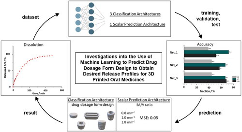
Three-dimensional (3D) printing, digitalization, and artificial intelligence (AI) are gaining increasing interest in modern medicine. All three aspects are combined in personalized medicine where 3D-printed dosage forms are advantageous because of their variable geometry design. The geometry design can be used to determine the surface area to volume (SA/V) ratio, which affects drug release from the dosage forms. This study investigated artificial neural networks (ANN) to predict suitable geometries for the desired dose and release profile. Filaments with 5% API load and polyvinyl alcohol were 3D printed using Fused Deposition Modeling to provide a wide variety of geometries with different dosages and SA/V ratios. These were dissolved in vitro, and the API release profiles were described mathematically. Using these data, ANN architectures were designed with the goal of predicting a suitable dosage form geometry. Poor accuracies of 68.5% in the training and 44.4% in the test settings were achieved with a classification architecture. However, the SA/V ratio could be predicted accurately with a mean squared error loss of only 0.05. This study shows that the prediction of the SA/V ratio using AI works, but not of the exact geometry. For this purpose, a global database could be built with a range of geometries to simplify the prescription process.

Graphical Abstract

Keywords:

• Artificial Neural Network
• artificial intelligence
• FDM 3D printing
• drug dissolution
• geometry design
• drug dosage form prediction

1. Introduction

Artificial intelligence (AI) and precision medicine are two important aspects of modern medicine. Both promise to revolutionize healthcare worldwide (Ashley 2016; Hodson 2016; Deng et al. 2021; Johnson et al. 2021; Maceachern and Forkert 2021). With precision medicine, which aims to personalize therapy for individuals, several approaches are utilized to stratify patient groups. For example, the genome has been examined to characterize disease risks and responses to treatment because of its genetic layout, environmental influences, and other characteristics (Jorgensen et al. 2019; Uddin et al. 2019). By cross-referencing with databases, a diagnosis can be made quickly and specifically, and appropriate therapy with the correct dosage and dosing regimen can be established. Owing to the digitalization of health-related data and the rapid proliferation of technologies across countries, changes and progress in the development and use of AI in healthcare are driven (Topol 2019). Despite the promised advantages, modern electronic medicine faces some challenges, such as data integrity and safety, privacy, bias, and model performance. Nevertheless, the field of AI in medicine is growing; in screening, diagnostics, prevention, therapy, and aftercare, databases are used to monitor processes, detect trends at an early stage, and react to them. For example, AI can support medical diagnostics by analyzing image data. Based on existing images and associated diagnoses, AI recognizes patterns in the image that are assigned to disease patterns. The analysis and availability of large amounts of data make it possible to recognize pathological changes in the image quickly and reliably, to adapt therapies individually to the patient, and to provide prognoses for further disease progression (Lundervold and Lundervold 2019; Schork 2019; Deng et al. 2021). The use of AI is also becoming increasingly prevalent in pharmaceutical research. Groups are identifying new chemical structures with desired properties based on large datasets and algorithms, which is accelerating the development of new drugs and helping fight diseases (Baskin et al. 2016; Paul et al. 2021; Karthikeyan and Priyakumar 2022). AI is also helpful in the development of dosage forms, as experimental work, cost, and time can be saved. It can provide support for formulation development, stability testing, and release characterization, as well as optimizing the manufacturing process (Madzarevic et al. 2019; Yang et al. 2019; Elbadawi et al. 2020; Muñiz Castro et al. 2021). Obeid et al. predicted the diazepam release behavior of 3D printed tablets with the input parameters infill density and surface area to volume (SA/V) ratio (Obeid et al. 2021). A similar approach has been adopted by Benkö et al., Stanojevic et al. and Madzarevic et al. in their studies. Based on the geometries of the dosage forms, used excipients, and active pharmaceutical ingredient (API) load, the respective release profiles were predicted (Madzarevic et al. 2019; Stanojević et al. 2020; Benkő et al. 2022). Elbadawi et al. developed a web-based pharmaceutical software ‘M3diseen’ to predict the 3D printability of medicines for fused deposition modeling (FDM) (Elbadawi et al. 2020). The filaments required for FDM printing are produced using hot-melt extrusion (HME). As HME is a complicated process in which the optimization of the fabrication parameters requires a lot of time and knowledge, the software predicts key fabrication parameters for printability and filament properties.

3D printing is particularly suitable for personalized medicine and is currently being researched in detail for this purpose (Goyanes et al. 2014; Goyanes et al. 2015; Fina et al. 2017; el Aita et al. 2020; Rahman and Quodbach 2021). Relevant processes are being investigated and potential polymers are being tested and developed (Gottschalk et al. 2021; Chamberlain et al. 2022). FDM 3D printing enables the manufacturing of a variety of geometries through the layer-by-layer construction of dosage forms. The geometries can have a bespoke pore structure, built-in cavities, as well as shapes that are not attainable via tablet compression. With FDM, the patient’s requirements can be precisely addressed. Limitations are given here by the properties of the polymers (e.g. swelling behavior, solidification behavior) and the swallowability of the individual geometry. FDM 3D printing is only suitable for smaller batches, because so far usually only one to two print heads work in parallel and the printing of one tablet, depending on the size, can take about 1 min. Especially for tailored medicine, 3D printing processes offer the advantage that geometries can be freely selected and designed. Adjustment of dosages and SA/V ratios can lead to the modification of the release rates (Sadia et al. 2018; Windolf et al. 2021; Windolf et al. 2022). Besides the individual dosage, it is of equal importance in personalized medicine that the duration of action and the onset of the effect are in line with the therapy and support compliance. This means that symptoms can be alleviated immediately with a rapid onset of action. But in the same way, with a prolonged release time, the effect can be sustained over a period of time, thus extending the ingestion intervals of the medicine. Due to the small batch sizes, non-destructive quality control processes and predictive tools are of interest. Therefore, AI technologies are used in this area to make predictions about the characteristics of the dosage form based for example on the formulation or geometry design.

In addition to the predictions of the resulting release profiles (Hassanzadeh et al. 2019), there are already a few approaches to predicting the design of the dosage form using an ANN (Novák et al. 2018; Grof and Štěpánek 2021). A computational design method for finding the internal structures for multi-component tablets that result in a preferred dissolution profile was developed by Grof and Štěpánek 2021.

Once the required API dose is known and the necessary release profile from the dosage form to achieve maximum therapeutic efficacy, reduce side effects, and increase compliance, an appropriate 3D printed dosage form geometry must be selected. In this study, the underlying geometry should be predicted to result in a predetermined dissolution profile with a given API load. This could streamline the workflow from prescription to 3D-printed tablets. Prediction by ANN is intended to bypass the design step that currently must be performed by skilled personnel, thus eliminating potential errors, and saving cost and effort. Previous studies have shown that the release behavior is independent of geometry and depends only on the SA/V ratio of the dosage form (Reynolds et al. 2002; Goyanes et al. 2015; Windolf et al. 2021; Windolf et al. 2022). Based on the generated release data for different SA/V ratios, the associated dissolution profile can be predicted using mathematical equations such as the Peppas Sahlin equation (Windolf et al. 2021). In the first approach, an ANN should be created to predict the geometry from the input data of the release curve and the desired API content. The predicted geometry should include the necessary SA/V ratio, which reflects the desired drug load in volume and ensures the release progression through the SA/V ratio. Subsequently, another neural net was created to backtrack the attempt, in which an appropriate SA/V ratio should be predicted for the desired curve.

2. Materials and methods

2.1. Materials

The formulation consisted of 5% (w/w) pramipexole dihydrochloride monohydrate (PDM, Chr. Olesen, Denmark) as a readily soluble API of the biopharmaceutics classification system (BCS) class I (Łaszcz et al. 2010; Komal et al. 2019; Tzankov et al. 2019). Mannitol (Parteck M^®, Merck, Germany) was used as a plasticizer at 10% (w/w) content. Polyvinyl alcohol (84%, PVA, Parteck MXP^®, Merck, Germany) was selected as a polymer. To improve flowability, 1% fumed silica (Aerosil^® 200 VV Pharma, Evonik, Germany) was added to the formulation. This formulation has been used in previous studies (Windolf et al. 2021; Windolf et al. 2022).

2.2. Methods

2.2.1. Hot-melt extrusion

The drug-containing filament was produced via HME with a co-rotating twin-screw extruder (Pharmalab HME 16, Thermo Fisher Scientific, USA) using an in-house manufactured die with a diameter of 1.85 mm. The feed rate was set to 5 g/min and the screw speed to 30 rpm. The temperatures of the heating zones as well as the screw configurations are shown in Table 1. The filaments were hauled off with a winder (Model 846700, Brabender, Germany) at a speed of 1.8 m/min to a target diameter of 1.75 mm. The diameter was controlled in-line using a laser-based diameter measurement module (Laser 2025 T, Sikora, Germany).

Table 1. Extrusion data (temperature profile and screw configuration).

Temperature profile in zone 1-10 / °C
zone / -	2	3	4	5	6	7	8	9	10
temperature / °C	30	100	180	180	180	180	180	195	195
screw configuration (die - gear)
die − 10 CE 1 L/D – KZ: 5 × 60°-3 × 30°- 5 CE 1 L/D- KZ: 4 × 90°-5 × 60°-3 × 30°- 10 CE 1 L/D − 2 CE 3/2 L/D – gear
CE = conveying element KZ = kneading zone

2.2.2 3D Printing of geometries

The drug-loaded filament was printed on a FDM 3D printer (Prusa i3 Mk3, Prusa Research, Czech Republic) into dosage forms with various geometries. These forms were designed by considering the SA/V ratio using the computer-aided design (CAD) software Fusion 360^® (Autodesk, USA) and were sliced in PrusaSlicer^® (Prusa Research, Czech Republic) to obtain the desired G-code. The printing temperature for the filament was 185 °C, the bed temperature was 60 °C, and printing speed was 20 mm/s. The infill percentage was 100%, printed in a concentric shape. In total, 196 different geometries were printed.

2.2.3. Description of the geometries for dataset

The printed geometries were numerically described as accurately as possible for processing using ANN. The parameters recorded were surface area (SA), volume (V), SA/V ratio, total weight, and API mass (mg total and mg API), layer height (lh), and extrusion width (ew) as printing parameters, number of layers in total, length, height, and width of the 3D geometry, as well as the diameter of pores and their surface area, amount of beam-layers, their height, and amount of cylinders/hollow cylinders connected by the beams (see Figure 1). Numbers were used for the fundamental geometric shapes, i.e. cylinder =1, hollow cylinder =2, pyramid =3 (Table 2).

Figure 1. Example for description of the geometries for dataset. Variation of cylindrical shaped tablet. SA: surface area; V: volume; lh: layer height; ew: extrusion width.

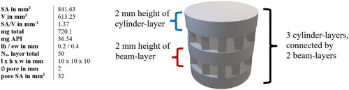
Table 2. Categorization of printed geometries.

Number	Name	Shape Examples
1	Cylinder
2	Hollow Cylinder
3	Pyramid
4	Double HollowCylinder
5	Hollow Cylinder with included Cylinder
6	Oblong
7	Spiral
8	Rectangle
9	Cuboid
10	Hollow Oblong
11	Egg-shaped
12	Hexagon

The amount of API contained covered a range of 1.7 − 49.2 mg. For each API content, a spectrum of SA/V ratios was attempted to be printed from the lowest possible to the highest possible SA/V using different designs (Figure 2). This was restricted by the limits that the forms should serve as oral dosage forms and, thus, be swallowable. For example, for a geometry with 2 mg of API, it was only possible to achieve 1.6 mm⁻¹ as the smallest SA/V ratio (egg-shaped). The higher the volume (more API), the larger the geometries could become and, thus, the SA/V ratio is smaller. With 10 mg API, for example, a range of 0.9–2.5 mm⁻¹ SA/V ratio could be covered. With an API load of 20–39 mg, the maximum achievable SA/V ratio was only 2 mm⁻¹, as the volume was too large and a correspondingly large surface area led to very large tablets, which in turn are difficult to swallow (Figure 3). The focus was on ingestible shapes (round and oval), but to cover a wider range, several geometries not suitable for ingestion (e.g. cuboid and pyramid) were also printed.

Figure 2. Distribution of API load (1.7 – 49.2 mg) and SA/V ratio (0.6 – 6.0 mm⁻¹) of printed geometries.

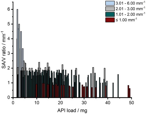
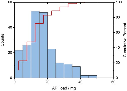
Figure 3. Quantity distribution of the printed tablets regarding the API content, n = 196. Blue columns: absolute counts; red line: cumulative percent (We refer the reader to the online version for the color coded graphs).

2.2.4. Dissolution test

According to the European Pharmacopoeia (Ph. Eur.) monographs 2.9.3 and 5.17.1 (European Pharmacopoeia Commission 2.9.3 2020; European Pharmacopoeia Commission 5.17.1 2020), release studies (n = 3–9) were performed with the basket method (Method 1) in a dissolution tester (DT 726, Erweka, Germany). The baskets were 3D printed from water-insoluble polylactide acid (PLA). They had to be adapted for printed tablets since the mesh size of the regular Ph. Eur. baskets is small (0.36−0.44 mm) and the baskets were clogged by the swollen polymer of the PVA formulation. This affected the hydrodynamic medium flow around the printed oral dosage forms. The self-printed baskets have the same outer dimensions as the Ph. Eur. baskets except that the mesh width was changed to 3 mm. The dissolution test for PDM-containing tablets was performed in 500 mL of degassed 0.1 N hydrochloric acid at pH 1.2 under sink conditions (c_s ≥200 mg/mL (Tzankov et al. 2019); maximum achieved concentration 0.1 mg/mL) and stirred at 50 rpm at a temperature of 37 ± 0.5 °C. The released API was measured using a UV-Vis spectral photometer (UV-1800 Shimadzu, Japan) at a wavelength of 263 nm. Samples were taken every 5 min for the first 30 min, then every 10 min for the next 90 min, followed by sampling in 20 min intervals. After a release time of 240 min, samples were taken every 30 min. A total of 1001 single dissolution curves were measured (n = 3–9 for each geometry).

2.2.5. Description of the dissolution curves

For the data input, the release curves were saved in an array with the released percentage of API over time. The dissolution profiles were also described with the Mean Dissolution Time (MDT, Equation 1(1) $$\mathrm{MDT}\mathrm{ }=\frac{\mathit{ABC}}{c_{\mathrm{\infty }}}=\mathrm{ }\frac{\sum _{i=o}^{\mathrm{\infty }}\left[\right(c_{i+1}-c_i)\times \frac{\left(t_i+t_{i+1}\right)}{2}]}{c_{\mathrm{\infty }}}$$(1) ), t_50% (time in which 50% API were released), t_80%, t_100%. (1) $$\mathrm{MDT}\mathrm{ }=\frac{\mathit{ABC}}{c_{\mathrm{\infty }}}=\mathrm{ }\frac{\sum _{i=o}^{\mathrm{\infty }}\left[\right(c_{i+1}-c_i)\times \frac{\left(t_i+t_{i+1}\right)}{2}]}{c_{\mathrm{\infty }}}$$(1) $\mathbf{MDT}$ indicates the average time an API molecule remains in a dosage form during release. The $\mathbf{MDT}$ (min) is calculated from the $\mathbf{ABC}$ (area between the curves) via the trapezoidal equation. ${\mathbf{c}}_{\mathbf{\infty }}$ represents the initial amount of API in the dosage form. ${\mathbf{c}}_{\mathit{i}}$ is the concentration of the API released over time (Costa and Sousa Lobo 2001; Tanigawara et al. 1982).

When dissolution data showed linear regions, the slope of these regions was also recorded as potential input parameter for analysis. In previous publications, it has been described that the release profile of the used formulation can be expressed with the Peppas Sahlin equation (Equation 2(2) $$\frac{{\mathrm{M}}_{\mathrm{t}}}{{\mathrm{M}}_{\mathrm{\infty }}}={\mathrm{k}}_1\times {\mathrm{t}}^{\mathrm{n}}+{\mathrm{k}}_2\times {\mathrm{t}}^{2\mathrm{n}}$$(2) ). Therefore, the descriptive parameters k₁, k₂, and n were calculated for the individual curves and also included in the dataset. (2) $$\frac{{\mathrm{M}}_{\mathrm{t}}}{{\mathrm{M}}_{\mathrm{\infty }}}={\mathrm{k}}_1\times {\mathrm{t}}^{\mathrm{n}}+{\mathrm{k}}_2\times {\mathrm{t}}^{2\mathrm{n}}$$(2)

The exponent $\mathbf{n}$ is the diffusion exponent for any geometric shape. The constants ${\mathbf{k}}_1,$ ${\mathbf{k}}_2$ describe the kinetics for erosion and diffusion (Siepmann and Peppas 2001; Windolf et al. 2021).

2.2.6. Dataset for ANN

A dataset was generated from the designed geometries (Section 2.2.3) and release curves (Section 2.2.5). A part of the dataset was already used in some previous studies (Windolf et al. 2021; Windolf et al. 2022). As different numbers of experiments (n = 3 – 9) were executed for each geometry, the dissolution curves were averaged to obtain a mean curve for each printed tablet. While originally 12 different geometry categories were printed (Section 2.2.3, Table 2), the classes were limited to less refined categories: ‘cylinder’, ‘hollow cylinder’, ‘oblong’ and ‘other’. The class ‘other’ was created so it was possible to use input data of unusual geometric shapes such as rectangular or spiral shapes while retaining the complexity of the overall classification problem. The problem gets more difficult if more classes of fewer examples are introduced and therefore the creation of the ‘other’ class was accepted as a compromise between complexity and the obtainable information and variance from unusual geometries. Tablets with large surface areas lead to large tablets that are difficult to swallow and additionally, the release curves no longer differ strongly with increasing SA/V ratio (Windolf et al. 2021). Therefore, tablets with large SA/V ratios were removed from the dataset, where outliers were defined by the interquartile range (IQR) of the SA/V ratio where $q_n(0.75),$ $q_n(0.25)$ describe the upper quartile (75%) and lower quartile (25%) respectively (Dekking and Kraaikamp 2005) (Equation 3(3) $$\mathit{IQR}\mathrm{ }=\mathrm{ }{q}_n\left(0.75\right)\mathrm{ }-\mathrm{ }{q}_n\left(0.25\right)$$(3) ). (3) $$\mathit{IQR}\mathrm{ }=\mathrm{ }{q}_n\left(0.75\right)\mathrm{ }-\mathrm{ }{q}_n\left(0.25\right)$$(3)

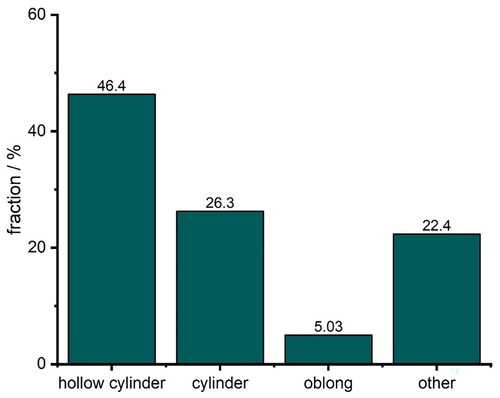
Each tablet with a SA/V ratio that was below $q_n(0.25) - 1.5 \mathit{IQR}$ and above $q_n(0.75) + 1.5 \mathit{IQR}$ was considered an outlier and removed from the dataset as proposed in the literature (Tukey 1977). Although this is a simple approach to classify outliers, we consider it sufficient for this application. Based on the IQR of the SA/V ratio, tablet geometries that represent SA/V ratios above 2.97 mm⁻¹ were excluded. Removal of outliers and deletion of replicates resulted in a dataset consisting of 179 distinct data points, each representing a geometry. The dataset is significantly imbalanced: The most prevalent class is hollow cylinder making up 46.4% of the tablets or 83 geometries in total, while only 5% (9 geometries) of the dataset are oblong-shaped tablets (Figure 4). The imbalance results from the fact that the data were first used for other studies (Windolf et al 2021; Windolf 2022) and some forms are particularly suitable for representing different volumes and surface areas without the geometries becoming too large and thus ‘unswallowable’. This must be considered during the training process and when assessing the performance of the classifier. The term ‘classifier’ is interchangeably used with ‘neural network’ in this study to describe the proposed architectures in the next section that are used to classify the input data into the underlying geometric shape. If the performance of the classifier is below 46.4% it can be considered unsuitable because any classifier that predicts the most prevalent class, i.e. hollow cylinder, every time, is equally good. Therefore 46.4% should be considered as a lower threshold for accuracy in this setting.

Figure 4. Class imbalance of 3D printed geometries. Hollow cylinder: 46.4%; cylinder: 26.3%; oblong: 5.0%; other: 22.4%.

2.2.7. Neural Network architectures

Artificial Neural Networks (ANN) are at the heart of most modern Machine Learning applications and connect input data to output data. ANN only provides the net architecture composed of different numbers of input and output neurons and different layers, while the specific weights and biases are computed by error backpropagation as an optimization method (Bishop 2006). The term ‘layers’ generally refers to a specific computational function, which is directly applied to the original input data or to the output of a different layer. The latter implies, that layers can be stacked and that the stack of layers constitutes the ANN architecture. The goal is to minimize a loss function so that the neural net provides concise output predictions when receiving appropriate input data. In this paper, ANNs were leveraged for two optimization goals: geometry classification and SA/V ratio prediction. For classification, three different architectures are investigated. The first architecture and most basic approach consisted of 7 linear layers, 2 dropout layers, 6 applications of batch normalization and exponential linear units (ELU) as nonlinear activation functions and each computational unit has a different purpose. Linear layers are one of the basic building blocks of most simple feed-forward neural network architectures and represent a linear transformation of the input vector (Bishop 2006). Applying a linear transformation to the input vector yields an output vector, where the output size of this transformation is a freely adjustable parameter. Linear layers can be thought of as calculating a matrix-vector multiplication first and then adding a bias term to the result (Bishop 2006). Because the weights (i.e. the entries of the matrix) are optimized through error backpropagation, linear layers with reduced output size can represent a lower-dimensional transformation of the input with a (potentially) reduced loss. Dropout layers act as regularization in deep neural networks and are often used to avoid overfitting where robustness is achieved by randomly dropping neuronal connections of the network (Srivastava et al. 2014). The fraction of discarded connections is controlled through a parameter $p,$ which is also freely adjustable (Srivastava et al. 2014). Another technique in machine learning is batch normalization which leads to faster convergence while also acting as a regularization (Ioffe and Szegedy 2015). The idea is to apply both rescalings and mean shifting to every output dimension of a certain layer (Ioffe and Szegedy 2015). The training inputs for ANNs are often processed in batches (or mini-batches), which correspond to a fixed number of training examples (Ioffe and Szegedy 2015). The statistical properties of those batches such as the mini-batch variance and the mini-batch mean are used for the rescaling and the mean shifting respectively, resulting in normalized values between 0 and 1 for the certain layer (Ioffe and Szegedy 2015). Another key component of every neural network architecture is the concept of a nonlinear activation function. In multilayer neural network architectures, nonlinear activation functions are necessary. Otherwise, multiple linear layers collapse into a single linear layer if they are stacked together without some form of nonlinearity (Bishop 2006). If no nonlinear activation functions are implemented between linear layers, the neural net will result into a simple linear matrix-vector product with a bias component. These functions are therefore required for every multilayer perceptron to become ‘universal approximators’ (Bishop 2006). ELU layers were used as nonlinear neuron activation functions, which were first introduced by Clevert at al (Clevert et al. 2016). and represent a less known variant of the Rectified Linear Unit (RELU). Instead of setting negative inputs to zero, the ELU layer interpolates for $x\le 0.$ In other cases, the activations are the same as for the RELU layer, shown in Equation 4(4) $$\mathit{ELU}\left(x\right)=\{\mathrm{ }\begin{array}{c}x,\mathit{\text{ if x}}>0\\ \alpha *\left(\exp \left(x\right)-1\right),\mathit{\text{ if x}}\le 0\end{array}$$(4) . (4) $$\mathit{ELU}\left(x\right)=\{\mathrm{ }\begin{array}{c}x,\mathit{\text{ if x}}>0\\ \alpha *\left(\exp \left(x\right)-1\right),\mathit{\text{ if x}}\le 0\end{array}$$(4)

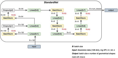
The hyperparameter $\alpha$ is frequently set to 1, which is also the default in this work. Both RELU and ELU activations are the same for $x>0.$ However, the ELU activation is smoother for negative values. The first architecture is named ‘StandardNet’ and is depicted in Figure 5. The net receives a total of 132 features consisting of the dissolution data (128 features) and the four inputs ‘mg API’, as well as ‘k₁’, ‘k₂’ and ‘n’ from fitting with the Peppas Sahlin equation. The input is passed in batches of 32 through the fully connected layer fc1 which outputs a 64-dimensional representation. Subsequently, batch normalization and the nonlinear ELU activation layer are applied. Note that neither the batch normalization nor the nonlinear activation changes the output dimension. In the next step, the output is passed through the first dropout layer with dropout probability p1, which is determined by hyperparameter optimization. The stack consisting of a fully connected layer, batch normalization, ELU, and dropout is repeated with an output dimension set to 32. This is the last application of dropout and in the next steps, the data is only passed through 4 stacks of fully connected layers, batch normalization and ELU where the output dimensions are 16, 8, 6 and 6. This output is processed by the last linear layer fc7, where the output dimension is set to the number of distinct geometry shapes (in this case 4 shapes). From this output that indicates the predicted class labels, the cross-entropy loss is calculated to obtain the gradient, which is passed on to the optimizer.

Figure 5. Architecture of StandardNet. B is the number of training examples, that are processed in parallel (batch size). The fc abbreviation in the linear layers stands for fully connected, which is a synonym for linear layers. ELU stands for exponential linear units and is the nonlinear activation function introduced in 2.2.7. mg API is the abbreviation of the drug amount and k₁, k_2, and n are descriptive parameters of the Peppas Sahlin equation (Equation 2(2) $$\frac{{\mathrm{M}}_{\mathrm{t}}}{{\mathrm{M}}_{\mathrm{\infty }}}={\mathrm{k}}_1\times {\mathrm{t}}^{\mathrm{n}}+{\mathrm{k}}_2\times {\mathrm{t}}^{2\mathrm{n}}$$(2) ).

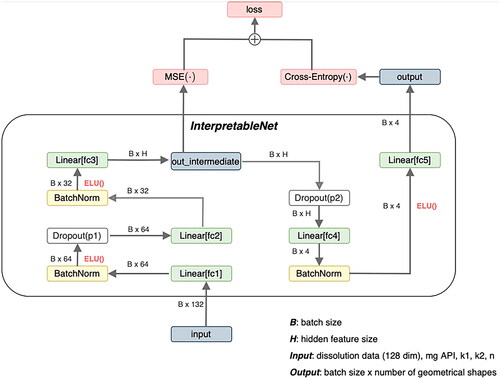
The second architecture which is called ‘InterpretableNet’ can be seen in Figure 6. The conceptual difference between the previous and this architecture is that certain tablet characteristics such as SA/V Ratio, surface area, volume, inner diameter, and mean dissolution time (MDT) should be predicted from the desired dissolution characteristics, the required drug amount (mg API) and the mentioned dynamical parameters of the Peppas Sahlin equations. These predictions are used within the same net to obtain a score for each tablet geometry. This score is used to predict the corresponding geometrical shape.

Figure 6. Architecture of InterpretableNet. B is the number of training examples, that are processed in parallel (batch size). The fc abbreviation in the linear layers stands for fully connected, which is a synonym for linear layers. ELU stands for exponential linear units and is the nonlinear activation function introduced in 2.2.7. mg API is the abbreviation of the drug amount and k₁, k_2, and n are descriptive parameters of the Peppas Sahlin equation (Equation 2(2) $$\frac{{\mathrm{M}}_{\mathrm{t}}}{{\mathrm{M}}_{\mathrm{\infty }}}={\mathrm{k}}_1\times {\mathrm{t}}^{\mathrm{n}}+{\mathrm{k}}_2\times {\mathrm{t}}^{2\mathrm{n}}$$(2) ). MSE refers to the mean-squared-error loss (Equation 6(6) $$\mathit{MSE}\mathrm{ }=\mathrm{ }\frac{1}{N}\sum _{n=1}^N{\left({\widehat{y}}_n-y_n\right)}^2$$(6) ).

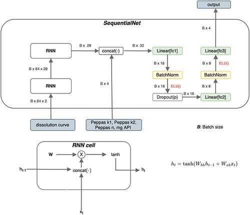
The last architecture that was used as a classifier exhibits the sequential and time-dependent nature of the dissolution curve and is referred to as ‘SequentialNet’ (Figure 7). It is composed of two stacked Recurrent Neural Networks (RNN) and the same stack of layers which were already described before in Figure 5. RNN are a common way to address time dependency by utilizing hidden states. These hidden states can represent connections to previous states of the system and can act as a memory (Elman 1990). The used RNN architecture was a simple Elman Net (Elman 1990). The dissolution curve is first passed through the two stacked RNN and the resulting representation of this curve is concatenated with the Peppas Sahlin coefficients and with the desired drug amount. In the previous architecture, the curve was passed along with these coefficients in the first place.

Figure 7. Architecture of SequentialNet. B is the number of training examples, that are processed in parallel (batch size). The fc abbreviation in the linear layers stands for fully connected, which is a synonym for linear layers. ELU stands for exponential linear units and is the nonlinear activation function introduced in 2.2.7. mg API is the abbreviation of the drug amount and k₁, k_2, and n are descriptive parameters of the Peppas Sahlin equation (Equation 2(2) $$\frac{{\mathrm{M}}_{\mathrm{t}}}{{\mathrm{M}}_{\mathrm{\infty }}}={\mathrm{k}}_1\times {\mathrm{t}}^{\mathrm{n}}+{\mathrm{k}}_2\times {\mathrm{t}}^{2\mathrm{n}}$$(2) ). h_t is the hidden state of the Recurrent Neural Network at time step t.

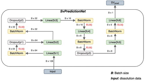
A neural net that should predict the SA/V ratio given the dissolution data was also constructed. SvPredictionNet is similar to the StandardNet and is shown in Figure 8.

Figure 8. Architecture of SvPredictionNet. B is the number of training examples, that are processed in parallel (batch size). The fc abbreviation in the linear layers stands for fully connected, which is a synonym for linear layers. ELU stands for exponential linear units and is the nonlinear activation function introduced in 2.2.7. SV_pred is the predicted surface-area-to-volume-ratio.

2.2.8. Loss Functions and hyperparameter optimization

Loss functions are functions that are commonly used to compare the values predicted by neural nets to the prior known ground truth scalar values or class labels. Assume that $\mathrm{y}$ is the true vector of class labels of size $\mathrm{C},$ where $C$ is the number of distinct classification labels. Furthermore, let $\mathrm{x}$ be the output of the last layer of some neural net, where $\mathrm{x}$ is a matrix with dimensions N × C $N \times C$ and $\mathrm{N}$ is the number of training inputs the neural net receives per forward pass (batch size). Then, for a single training input $\mathrm{i}$ the following is true (Bishop 2006; Sammut and Webb 2010) (Equation 5(5) $$l_n=\mathrm{ }-\text{ log }\frac{\exp \left(x_{n,y_n}\right)}{{\sum }_{c=1}^C\exp \left(x_{n,c}\right)}\mathrm{ }\mathit{for}\mathrm{ }n=1,\dots ,\mathrm{ }N$$(5) ): (5) $$l_n=\mathrm{ }-\text{ log }\frac{\exp \left(x_{n,y_n}\right)}{{\sum }_{c=1}^C\exp \left(x_{n,c}\right)}\mathrm{ }\mathit{for}\mathrm{ }n=1,\dots ,\mathrm{ }N$$(5) where the total loss $l (x,y)$ is obtained by calculating the average over each $l_n$ from $1$ to $N.$ The cross-entropy loss is used within the classification task in the StandardNet, InterpretableNet, and SequentialNet to compare the class label predictions to the ground truth class labels. To control for the class imbalance, which was mentioned in 2.2.6, the loss of a particular prediction was weighted with a weight function that takes the skewed distribution of each subclass into account. The reciprocal of the relative frequency of each class was used as a weight function (Sammut and Webb 2010), which results in low weights for frequent classes such as hollow cylinder and higher importance for less common classes (e.g. oblong class). This implicitly sets the focus on the least frequent classes which often leads to better results for these classes. The other loss function is the commonly used mean squared error loss (MSE). Let $\widehat{y}$ be a N-dimensional vector that contains scalar predictions of the ground truth values $y.$ Then, the total MSE loss is calculated via Equation 6(6) $$\mathit{MSE}\mathrm{ }=\mathrm{ }\frac{1}{N}\sum _{n=1}^N{\left({\widehat{y}}_n-y_n\right)}^2$$(6) (Sammut and Webb 2010). (6) $$\mathit{MSE}\mathrm{ }=\mathrm{ }\frac{1}{N}\sum _{n=1}^N{\left({\widehat{y}}_n-y_n\right)}^2$$(6)

The MSE loss is used to assess the predictive performance of the SvPredictionNet. The hyperparameters, such as the dropout probability $p$ and the learning rate, were optimized with the help of pytorch (Paszke et al. 2019) and optuna (Akiba et al. 2019).

3. Results and discussion

The used architectures can be categorized into two broad categories: classification architectures that should predict the suitable geometric shape (StandardNet, SequentialNet, InterpretableNet) and a scalar prediction architecture that return the SA/V ratio as a continuous positive value (SvPredictionNet). Accuracy is only meaningful in the context of classification architectures as this term is often considered as the ratio between correctly predicted classes and the total number of samples. Therefore, accuracy measures are only provided for StandardNet, InterpretableNet and SequentialNet and in the case of the SvPredictionNet architecture we refer to the loss metric described in Section 2.2.8. The dataset was split into training, validation, and test set, where 80% of the data were used to train weights of the neural nets and 10% of the data were used for validation and test sets, respectively. Splitting the dataset into these three sets is standard practice and results in less biased and more accurate estimators for the reported accuracies and loss metrics. The additional validation set is used to tune hyperparameters whereas the test set is utilized to obtain estimates of classifier performance for unseen data.

3.1. Prediction of the geometry from dissolution curves

To implement the goal of predicting geometries for 3D-printed drug dosage forms with desired release profiles, different networks were constructed. First, it was attempted to predict the form as accurately as possible with class labels (cylinder, hollow cylinder, etc.) and in the next step with exact diameter, height, width, number of pores, etc., to reproduce the appearance of a possible geometry (Section 2.2.3, Figure 1). Since the SA/V ratio is set based on the release profile, the desired API content is given as additional information so that the volume is known, and the ANN can then output a suitable geometry for the desired volume and SA/V ratio.

Three networks were used for this approach, which was set up differently (2.2.7: StandardNet, InterpretableNet, SequentialNet). For each of the 90 epochs, Figure 9 shows both accuracies and losses of the classification architectures. Each epoch represents a complete pass of every training example through the ANN (Nielsen 2015). The neural nets StandardNet and InterpretableNet show a moderate acceleration of both training and validation accuracy along the increasing number of epochs.

Figure 9. Accuracy (left column) and loss (right column) for each epoch for classification networks. Red: validation; blue: training (We refer the reader to the online version for the color coded graphs).

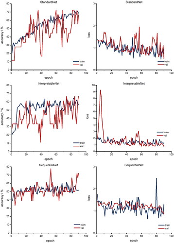
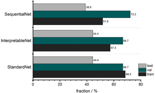
Furthermore, both validation and training loss also decreases over time for the StandardNet and the InterpretableNet. For the latter architecture, there is a pronounced peak in the validation loss around epoch 5. One possible explanation for this anomaly is the fact that the validation set was relatively small in absolute units (sample size 18), which may lead to unreliable loss estimates for some epochs. The fact that the validation loss reverts to its mean value in the 10^th epoch supports this consideration. The more sophisticated design of the SequentialNet did not result in better performance. Specifically, the training accuracy of the mentioned neural net is stuck in a tight channel between 40% and 60% and settles to 52% in the last epoch. In relation to the lower accuracy threshold of 46% (Section 2.2.6), this is not a considerable improvement compared to the complexity of the architecture. The peak in the corresponding loss plot is not surprising, as the loss acceleration coincides with a drop in training accuracy. Figure 10 depicts the final accuracies of the last epoch for the different classification architectures. The training performance is influenced by the architecture type: The training accuracy of the basic approach, which is implemented by the StandardNet, outperforms the other architectures by some margin. Indeed, the training accuracy of 68.5% is 11.2 percentage points higher than the InterpretableNet and 16.7 percentage points higher than the accuracy of the SequentialNet. This suggests that a simple approach is superior to either presupposing the features which should be extracted or leveraging more sophisticated architectures such as RNN. It also translates to the test set with an accuracy of 44.4% for the StandardNet architecture compared to 44.4% for the InterpretableNet, which were surprisingly identical. The SequentialNet reaches a test accuracy of 38.9%. These test results show that none of the three architectures generalizes well on unseen data. The performance on the validation set is different. In this case, SequentialNet achieves the best performance with an accuracy of 72.2%. Both other architectures are accurate in 66.7% of the cases. The higher performance can also be interpreted as an outlier: as the validation set and test set are small, a misclassification of just one sample has large effect on the accuracy (± 5.6 pp. accuracy for n = 18). It is important to emphasize that the amount of data which is available for the test and validation set can lead to unreliable results.

Figure 10. Accuracies for the last epoch for classification networks. Grey: test; green: validation; black: training (We refer the reader to the online version for the color coded graphs).

The StandardNet is the best overall choice among the three architectures that are used for classification as its usage combines a simple architecture with moderate results. However, the overall training accuracies imply that no architecture was able to correctly adapt to the data.

Unfortunately, it became clear that these ANN-Designs were not able to predict the required information accurately so that the appropriate geometry can be designed based on predicted data. Ideally, the network should be able to infer from the given information which class label, height, diameter, etc. is needed to create a geometry with desired volume and surface area. However, the class label, i.e. the appropriate geometry, must first be selected for this procedure, but the release curves do not allow the necessary geometry to be inferred exactly. At least it was evaluated to see if it could identify a trend based on the dissolution profile as to which geometry was suitable so that this form could be used as a basis for the patient.

3.2. Prediction of SA/V ratio from dissolution curves

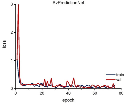
As the initial goal could not be attained, a different procedure was investigated. Since the release behavior is based on the SA/V ratio of the geometry, this ratio should be predicted from the given data, so that subsequently the appropriate geometry could be selected from a database. This could offer the advantage that several geometries available for selection could be chosen during this screening process and thus limitations, such as the swelling behavior of the polymers used, could also be taken into account. The database with possible geometries could be fed by different persons independent of location, it would only be necessary to specify the volume and the surface with the resulting SA/V ratio and possible pore sizes based on the polymer swelling behavior. To implement this concept, the prediction approach of Windolf et al. (2021) was used. In this study, a correlation between the MDT and the SA/V ratio and between the Peppas Sahlin equation and the SA/V ratio was used to predict the resulting release profile based on the SA/V ratio. This approach was reversed here to predict the SA/V ratio based on the dissolution curve. With this information, the required surface area could be calculated for a desired dose and a corresponding geometry could be designed with the CAD software, or chosen from a possible database. As a scalar prediction net architecture, the SvPredictionNet was used. The results in Figure 11 indicate that the net learns a reasonable representation from which predictive SA/V ratios are obtained. The model however does also suffer from an incapability to generalize well. While the overall test set MSE loss of 0.054 between predicted and ground truth is acceptable, there are some predictions that are off by a large margin, e.g. a predicted value of 1.44 mm⁻¹ with the ground truth value of 1.9 mm⁻¹, representing a squared error loss of 0.212. The inaccurate predictions for the test set are more common for geometries with higher SA/V ratios. For example, in 3 of 4 cases where the MSE was larger than 0.1, the SA/V ratios of the related tablets were larger than 2.3 mm⁻¹. This underlines the fact that acquiring more data is necessary for more reliable results, especially for dissolution curves where the underlying geometrical shapes represent higher SA/V ratios. The same argument can be made for the classification problem. As this problem is harder to solve than the prediction of SA/V ratios one would need at least as much data as for those.

Figure 11. Loss for SvPredictionNet. Red: validation; blue: training (We refer the reader to the online version for the color coded graphs).

4. Conclusion

In this study, four different approaches were pursued to use Machine Learning to make predictions for geometric designs suitable as oral dosage forms. The geometry should be designed with respect to its API content and desired release behavior. This would allow a prescription workflow to be established for 3D printed oral dosage forms. The approach of using the given data to predict a geometry with the required length, width, height, and underlying geometry such as a cylinder or hollow cylinder by an artificial neural network was unfortunately not possible. Therefore, a general approach was taken to predict only the geometry without exact dimensions from the available data. It was assumed that this would not work, since the shape should have little to no influence on the release profile. Nevertheless, the geometry corresponding to the dissolution curve could be predicted with an accuracy of 68.5% (training) and 44.4% (test). The generated accuracy was higher than expected. Another approach was to predict the required SA/V ratio for a given release profile. This was possible with a MSE loss of 0.05. With this procedure, the swelling behavior of the polymer can cause errors, since the digitally generated SA/V ratio can be affected in vitro by the swelling of pores and the release curves therefore do not match the generated SA/V ratio. Thus, studies on the swelling behavior of the polymer should be carried out in advance to ensure those properties do not falsify the data. Another strong influencing factor is the distribution of the data, which is unfortunately unevenly distributed due to the given constraints regarding swallowability in this study, making it difficult to predict the appropriate geometry. The scope of the study was limited to neural networks as a model architecture. It should be emphasized, that there are a lot of other different architectures and algorithms available. As all four approaches were either classification or regression setups, further studies for other algorithms such as Random Forest Classification or Random Forest Regression are left for future research. To take advantage of the opportunities 3D printing offers for personalized medicine, the geometry with the desired properties must still be created manually. Based on the SA/V ratio prediction and the desired API content, the required surface area and volume can be calculated, but the geometry containing these values must be created and tested manually, which in turn takes a lot of time and is prone to errors. To avoid having to perform these steps for every prescription, a database could be created with the associated surface area and volume information so that the required form only needs to be selected and printed. To create a working network for each formulation, much more data is needed, which is very unusual and uneconomical for the pharmaceutical field. For such an approach, a collaboration between multiple institutions that publish their geometries with associated release data and formulations is necessary. This way it might be possible to create a database to select the drug dosage from geometry. For the particular formulation used, the required SA/V ratio can be predicted via the manual route of Windolf et al. 2021 or a neural network as described in Section 3.2. In the future, a program with a user-friendly interface could be designed, which is connected to the geometry database and suggests geometries for the calculated SA/V ratio and desired dosage, and the pharmacist or physician could select the appropriate form tailored to the patient, which also takes into account the properties of the formulation, such as the swelling behavior so that no pores can swell and thus change the release profile by reducing the required surface area. However, this could provide a method to establish a prescription process of 3D printed dosage forms.

Acknowledgements

The authors want to thank Daniel Casper and Dr. Marcel Schweitzer for their help and input for ANN creation and optimization.

Disclosure statement

The authors report there are no competing interests to declare.

Data availability statement

The data that support the findings of this study are available from the corresponding authors, [HM, LE], upon reasonable request.

Additional information

Funding

This research was funded by Bundesministerium für Bildung und Forschung–Project ‘ProMat Leben–Polymere’ ‘PolyPrint’, Project no.: 13XP5064B.

References

- Akiba T, Sano S, Yanase T, Ohta T, Koyama M. 2019. Optuna: a next-generation hyperparameter optimization framework. In Ankur Teredesai, Vipin Kumar (General chairs), Proceedings of the 25th ACM SIGKDD International Conference on Knowledge Discovery & Data Mining New York, NY, USA: Association for Computing Machinery; p. 2623–2631.
- Ashley EA. 2016. Towards precision medicine. Nat Rev Genet. 17(9):507–522.
- Baskin II, Winkler D, Tetko I. v 2016. A renaissance of neural networks in drug discovery. Expert Opin Drug Discov. 11(8):785–795.
- Benkő E, Ilič IG, Kristó K, Regdon G, Csóka I, Pintye-Hódi K, Srčič S, Sovány T. 2022. Predicting drug release rate of implantable matrices and better understanding of the underlying mechanisms through experimental design and artificial neural network-based modelling. Pharmaceutics. 14(2):228.
- Bishop CM. 2006. Pattern recognition. Mach Learn. 128:225–284.
- Chamberlain R, Windolf H, Geissler S, Quodbach J, Breitkreutz J. 2022. Precise dosing of pramipexole for low-dosed filament production by hot melt extrusion applying various feeding methods. Pharmaceutics. 14(1):216.
- Clevert D-A, Unterthiner T, Hochreiter S. 2016. Fast and accurate deep network learning by exponential linear units (ELUs). ICLR. Vol. 1, p. 1–14.
- Costa P, Sousa Lobo JM. 2001. Modeling and comparison of dissolution profiles. Eur J Pharm Sci. 13(2):123–133.
- Dekking FM,Kraaikamp C, LHP, MLE., 2005. Exploratory data analysis: numerical summaries. In George Casella, Stephen Fienberg, Ingram Olkin (Adv.), A modern introduction to probability and statistics: understanding why and how. London: Springer London; p. 231–243. ISBN 978-1-84628-168-6.
- Deng J, Hartung T, Capobianco E, Chen JY, Emmert-Streib F. 2021. Editorial: artificial intelligence for precision medicine. Front Artif Intell. 4:834645.
- el Aita I, Breitkreutz J, Quodbach J. 2020. Investigation of semi-solid formulations for 3d printing of drugs after prolonged storage to mimic real-life applications. Eur J Pharm Sci. 146:105266.
- Elbadawi M, McCoubrey LE, Gavins FKH, Ong JJ, Goyanes A, Gaisford S, Basit AW. 2021. Harnessing artificial intelligence for the next generation of 3D printed medicines. Adv Drug Deliv Rev. 175:113805.
- Elbadawi M, Muñiz Castro B, Gavins FKH, Ong JJ, Gaisford S, Pérez G, Basit AW, Cabalar P, Goyanes A. 2020. M3DISEEN: a novel machine learning approach for predicting the 3D printability of medicines. Int J Pharm. 590:119837.
- Elman JL. 1990. Finding structure in time. Cognitive Science. 14(2):179–211.
- European Pharmacopoeia Commission 2.9.3 2020. Dissolution test for solid dosage forms. In European Pharmacopoeia; European Directorate for the Quality of Medicines & HealthCare of the Council of Europe (EDQM), Vol 10.2, p. 326–333.
- European Pharmacopoeia Commission 5.17.1 2020. Recommendations on Dissolution Testing. In European Pharmacopoeia; European Directorate for the Quality of Medicines & HealthCare of the Council of Europe (EDQM), Vol 10.2, p. 801–807.
- European Pharmacopoeia Commission 2020. Monograph pramipexole dihydrochloride monohydrate. In European Pharmacopoeia; European Directorate for the Quality of Medicines & HealthCare of the Council of Europe (EDQM), Vol 10.0, p. 5382–5384.
- Fina F, Goyanes A, Gaisford S, Basit AW. 2017. Selective laser sintering (sls) 3d printing of medicines. Int J Pharm. 529(1-2):285–293.
- Gottschalk N, Bogdahn M, Harms M, Quodbach J. 2021. Brittle polymers in fused deposition modeling: an improved feeding approach to enable the printing of highly drug loaded filament. Int J Pharm. 597:120216.
- Goyanes A, Buanz ABM, Basit AW, Gaisford S. 2014. Fused-filament 3D printing (3DP) for fabrication of tablets. Int J Pharm. 476(1-2):88–92.
- Goyanes A, Robles Martinez P, Buanz A, Basit AW, Gaisford S. 2015. Effect of geometry on drug release from 3D printed tablets. Int J Pharm. 494(2):657–663.
- Grof Z, Štěpánek F. 2021. Artificial intelligence-based design of 3D-printed tablets for personalised medicine. Comput Chem Eng. 154:107492.
- Hassanzadeh P, Atyabi F, Dinarvand R. 2019. The significance of artificial intelligence in drug delivery system design. Adv Drug Deliv Rev. 151-152:169–190.
- Hodson R. 2016. Precision medicine. Nature. 537(7619):S49–S49.
- Ioffe S, Szegedy C. 2015. Batch normalization: accelerating deep network training by reducing covariate shift. CoRR. abs/1502.03167. Vol. 37, p. 448–456.
- Johnson KB, Wei W, Weeraratne D, Frisse ME, Misulis K, Rhee K, Zhao J, Snowdon JL. 2021. Precision medicine, AI, and the future of personalized health care. Clin Transl Sci. 14(1):86–93.
- Jorgensen AL, Prince C, Fitzgerald G, Hanson A, Downing J, Reynolds J, Zhang JE, Alfirevic A, Pirmohamed M. 2019. Implementation of genotype-guided dosing of warfarin with point-of-care genetic testing in three UK clinics: a matched cohort study. BMC Med. 17(1):11.
- Karthikeyan A, Priyakumar UD. 2022. Artificial intelligence: machine learning for chemical sciences. J Chem Sci. 134(1):2.
- Komal C, Dhara B, Sandeep S, Shantanu D, Priti MJ. 2019. Dissolution-controlled salt of pramipexole for parenteral administration: in vitro assessment and mathematical modeling. Dissolution Technol. 26(1):28–35.
- Łaszcz M, Trzcińska K, Kubiszewski M, Kosmacińska B, Glice M. 2010. Stability studies and structural characterization of pramipexole. J Pharm Biomed Anal. 53(4):1033–1036.
- Lundervold AS, Lundervold A. 2019. An overview of deep learning in medical imaging focusing on MRI. Z Med Phys. 29(2):102–127.
- Maceachern SJ, Forkert ND. 2021. Machine learning for precision medicine. Genome. 64(4):416–425.
- Madzarevic M, Medarevic D, A Vulovic A, Sustersic T, Djuris J, Filipovic N, Ibric S. 2019. Optimization and prediction of ibuprofen release from 3D DLP printlets using artificial neural networks. Pharmaceutics. 11(10):544.
- Muñiz Castro B, Elbadawi M, Ong JJ, Pollard T, Song Z, Gaisford S, Pérez G, Basit AW, Cabalar P, Goyanes A. 2021. Machine learning predicts 3D printing performance of over 900 drug delivery systems. J Control Release. 337:530–545.
- Nielsen MA. 2015. Neural Networks and Deep Learning. San Francisco, CA: Determination Press, 25, p. 15–24.
- Novák M, Boleslavská T, Grof Z, Waněk A, Zadražil A, Beránek J, Kovačík P, Štěpánek F. 2018. Virtual prototyping and parametric design of 3D-printed tablets based on the solution of inverse problem. AAPS PharmSciTech. 19(8):3414–3424.
- Obeid S, Madžarević M, Krkobabić M, Ibrić S. 2021. Predicting drug release from diazepam fdm printed tablets using deep learning approach: influence of process parameters and tablet surface/volume ratio. Int J Pharm. 601:120507.
- Paszke A, Gross S, Massa F, Lerer A. 2019. PyTorch: an imperative style, high-performance deep learning library. Adv Neural Inf Process Syst. 32:8026-8037.
- Paul D, Sanap G, Shenoy S, Kalyane D, Kalia K, Tekade RK. 2021. Artificial intelligence in drug discovery and development. Drug Discov Today. 26(1):80–93.
- PyTorch Foundation - Crossentropyloss. https://Pytorch.Org/Docs/Stable/Generated/Torch.Nn.CrossEntropyLoss.Html. (assessed 15.05.2022)
- Rahman J, Quodbach J. 2021. Versatility on Demand – The case for semi-solid micro-extrusion in pharmaceutics. Adv Drug Deliv Rev. 172:104–126.
- Reynolds TD, Mitchell SA, Balwinski KM. 2002. Investigation of the effect of tablet surface area/volume on drug release from hydroxypropylmethylcellulose controlled-release matrix tablets. Drug Dev Ind Pharm. 28(4):457–466.
- Sadia M, Arafat B, Ahmed W, Forbes RT, Alhnan MA. 2018. Channelled tablets: an innovative approach to accelerating drug release from 3D printed tablets. J Control Release. 269:355–363.
- Sammut C, Webb G. 2010. Mean squared error. In Claude Sammut, Geoffrey I. Webb (Eds.), Encyclopedia of Machine Learning; Springer US: Boston, MA, p. 653. ISBN 978-0-387-30164-8.
- Schork NJ. 2019. Artificial intelligence and personalized medicine. Cancer Treat Res. 178:265–283.
- Siepmann J, Peppas NA. 2001. Modeling of drug release from delivery systems based on hydroxypropyl methylcellulose (HPMC). Adv Drug Deliv Rev. 48(2-3):139–157.
- Srivastava N, Hinton G, Krizhevsky A, Sutskever I, Salakhutdinov R. 2014. Dropout: a simple way to prevent neural networks from overfitting. J Mach Lear Res. 15:1929–1958.
- Stanojević G, Medarević D, Adamov I, Pešić N, Kovačević J, Ibrić S. 2020. Tailoring atomoxetine release rate from DLP 3D-printed tablets using artificial neural networks: influence of tablet thickness and drug loading. Molecules. 26(1):111.
- Tanigawara Y, Yamaoka K, Nakagawa T, Uno T. 1982. New method for the evaluation of in vitro dissolution time and disintegration time. Chem Pharm Bull. 30(3):1088–1090.
- Topol EJ. 2019. High-performance medicine: the convergence of human and artificial intelligence. Nat Med. 25(1):44–56.
- Tukey 1977. Chapter 2D: Fences, and outside values, Exploratory Data Analysis. In Frederick Mosteller (Ed.), Addison-Wesley Publishing Company, Reading, Mass 2:43–47. ISBN 0-201-07616-0.
- Tzankov B, Voycheva C, Yordanov Y, Aluani D, Spassova I, Kovacheva D, Lambov N, Tzankova V. 2019. Development and invitro safety evaluation of pramipexole-loaded hollow mesoporous silica (HMS) particles. Biotechnol Biotechnol Equip. 33(1):1204–1215.
- Uddin M, Wang Y, Woodbury-Smith M. 2019. Artificial intelligence for precision medicine in neurodevelopmental disorders. Npj Digit Med. 2(1)2019 2:1 :1–10.
- Windolf H, Chamberlain R, Quodbach J. 2021. Predicting drug release from 3D printed oral medicines based on the surface area to volume ratio of tablet geometry. Pharmaceutics. 13(9):1453.
- Windolf H, Chamberlain R, Quodbach J. 2022. Dose-independent drug release from 3D printed oral medicines for patient-specific dosing to improve therapy safety. Int J Pharm. 616:121555.
- Yang Y, Ye Z, Su Y, Zhao Q, Li X, Ouyang D. 2019. Deep learning for in vitro prediction of pharmaceutical formulations. Acta Pharm Sin B. 9(1):177–185.