Medium range sea ice prediction in support of Japanese research vessel MIRAI’s expedition cruise in 2018

ABSTRACT

The Japanese research vessel MIRAI sailed into the Arctic Ocean through the Bering Strait from 4 to 25 November 2018 to study the atmosphere, ocean, and sea ice of the Chukchi Sea. Early winter dynamics and thermodynamics can cause sea ice conditions to change over short timescales. Heavy ice pressure may build up in the compression of compact ice. MIRAI is an ice-strengthened ship that has to avoid thick sea ice and areas of high sea ice coverage, and therefore precise medium-range forecast of sea ice distribution is key to its safe and efficient navigation. A high-resolution (about 2.5 km) coupled ice–ocean model was used to produce medium-range (10-day) forecasts for the expedition. European Center for Medium-Range Weather Forecast’s atmospheric model high-resolution 10-day forecast was used as forcing data. Forecast skill is measured by ice edge error, which is the average distance between forecast and observed ice edges. Using a threshold of 15% sea ice concentration to indicate the ice edge, the maximum ice edge error in the ice–ocean coupled model in the Chukchi Sea is 16 km, indicating that the model is able to provide 10-day forecasts with sufficient accuracy for the vessel’s operation.

KEYWORDS:

• Sea ice forecasting
• numerical simulation
• Arctic Ocean
• shipping

1. Introduction

Global climate models and regional sea ice models have been employed to assess the predictability of Arctic sea ice on seasonal and decadal time scales (Kubat, Sayed, Savage, & Carrieres, 2010; Turnbull & Taylor, 2017) while a few studies have focused on shorter time scales (De Silva, Yamaguchi, & Ono, 2015; Inoue et al., 2015; Ono, Inoue, Yamazaki, Dethloff, & Yamaguchi, 2016; Schweiger & Zhang, 2015). Most of the available numerical models (Preller & Posey, 1989; Schweiger & Zhang, 2015) have shown high uncertainties in short-term (about 5-day) and regional predictions. Precise sea ice and ocean current predictions are vital for offshore oil and gas production, commercial fisheries, and commercial shipping in the Arctic Ocean. Therefore there is an urgent need for state-of-the-art operational forecasting systems with high accuracy to support the exploration of the Arctic.

A number of operational sea ice prediction models are currently available. One example is the Arctic Cap Nowcast/Forecast System (ACNFS) developed by the Naval Research Laboratory in the United States; it is a coupled ice–ocean forecast system with a resolution of 1/12° (Hebert et al., 2015). The Canadian Regional Ice Prediction System (RIPS; Buehner, Caya, Pogson, Carrieres, & Pestieau, 2013) also produces forecasts at a spatial resolution of 1/12° and a temporal resolution of 48 h. Another example is the TOPAZ4 system developed by the European Union; it is a coupled ocean–sea ice data assimilation system designed for the North Atlantic Ocean and the Arctic (Sakov et al., 2012) and uses the ensemble Kalman filter for data assimilation. Nakanowatari et al. (2018) found that for lead times of up to 3 days, the TOPAZ4 system could accurately predict summer sea ice distribution in the Eastern Siberian Sea. The UK Meteorological Office has developed a 10-day global ocean forecast and reanalysis system with a spatial resolution of 1/4°. The Operational Mercator global ocean forecast and analysis system has a resolution of 1/12°; it is also providing 10-day three-dimensional global ocean forecasts. Finally, the Baltic Sea Monitoring and Forecasting Centre (BAL MFC) produces 2-day sea ice forecasts with a spatial resolution of 2 km for the North Sea and Baltic Sea.

The medium range sea ice forecast of the Ice–Princeton Ocean Model (IcePOM) of the Laptev Sea reproduced satellite-derived sea ice extent reasonably well (De Silva et al., 2015); this is because of the improved expression of the ice–albedo feedback and ice–eddy interaction processes in the model. The model has specifically been designed to predict sea ice conditions in the marginal ice zone (MIZ) by explicitly treating ice floe collisions and mesoscale eddy activity. Therefore, it is one of the best candidates for operational sea ice forecasts in the MIZ.

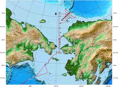
The Japanese RV MIRAI has been making sea ice and ocean observations in the Arctic Ocean since 1998. Prior to 2018, all cruises were conducted in summer and autumn. The first early winter cruise took place in 2018. Ship tracks and locations for conductivity, temperature and depth (CTD) observations for this cruise are shown in Figure 1.

Figure 1. Cruise tracks of the research vessel MIRAI in 2018 and locations for conductivity, temperature and depth (CTD) observations. Vertical profiles along track A–B are shown in Figure 7.

Because of the dynamics and thermodynamics of early winter, Arctic sea ice conditions can change over short timescales. Leads may open and close over a very short time, and heavy pressure may build up as compact ice is further compressed. These short-term and small-scale processes strongly influence shipping in ice-infested waters. The RV MIRAI is not an ice-class vessel and thus, has to avoid thick sea ice and areas of high sea ice coverage as much as possible. Therefore, precise medium range forecast of sea ice distribution is key to its safe and efficient navigation. The purpose of this study is to investigate the ability of models to produce medium range (10-day) sea ice forecasts in the Chukchi Sea with ice edge error of less than 20 km – an operational requirement of MIRAI. A coupled ice–ocean model with mesoscale eddy resolving abilities is used.

2. Model description and experimental design

The coupled ice–ocean model used in this study is based on the model developed by De Silva et al. (2015). The ocean model is based on generalized coordinates, the Message Passing Interface version of the Princeton Ocean Model (Mellor, Hakkinen, Ezer, & Patchen, 2002). The level-2.5 turbulence closure scheme of Mellor and Yamada (1982) is used for vertical eddy viscosity and diffusivity. Horizontal eddy viscosity and diffusivity are calculated using the formula of Smagorinsky (1963), which takes into account horizontal grid size, velocity gradients and a proportionality coefficient (a value of 0.2 is chosen for this study). The ice thermodynamics model is based on the zero-layer thermodynamic model proposed by Semtner (1976) and surface fluxes (shortwave radiation, longwave radiation, sensible heat flux, and latent heat flux) are calculated according to the bulk formulation proposed by Parkinson and Washington (1979). Snow effect is parameterized according to Zhang and Zhang (2001) where the fraction of precipitation that changes into snow is a linear function of air temperature; fraction is 1 when air temperature is below −5°C, fraction is 0 when air temperature is above 5°C, and fraction is between 0 and 1 when temperature is between −5 and 5°C. The ice rheological model is based on the elastic–viscous–plastic (EVP) rheology proposed by Hunke and Dukowicz (2002) and is modified to take into account ice floe collisions, following Sagawa and Yamaguchi (2006), Fujisaki, Yamaguchi, and Mitsudera (2010), and De Silva et al. (2015).

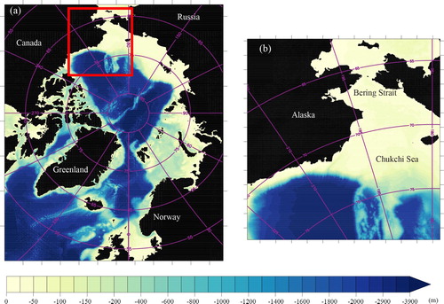
Figure 2 shows the model domains, which are constructed from the Earth Topography 1 arc-minute Gridded Elevation Dataset (ETOPO1). Zonal and meridional grid spacings are approximately 2.5 × 2.5 km for the high-resolution regional model (Figure 2(b)) and 25 × 25 km for the pan-Arctic model (Figure 2(a)). The vertical grid uses sigma coordinate systems with 33 levels. To resolve surface and bottom ocean dynamics, logarithmic distribution is used for the top ten and bottom three levels, and linear distribution is used for all other levels. At the model’s margins, a radiation-boundary condition is applied for the ocean part of the model, and an open-boundary condition is applied for the sea ice part of the model. In the Bering Strait boundary to the south, salinity and temperature are relaxed to the monthly mean of the Polar Science Center Hydrographic Climatology (PHC3.0) data (Steele, Morley, & Ermold, 2001). The inflow of Pacific water in the Bering Strait is set to an annual mean of 0.8 Sverdrup (1 Sv = 10⁶ m³ s⁻¹) and a seasonal amplitude of 0.4 Sv, with maximum inflow in June and minimum in December. Satellite observations of sea ice concentration are assimilated into IcePOM with the nudging method described by Mudunkotuwa, De Silva, and Yamaguchi (2016). They claimed that assimilating sea ice concentration improved the ocean (salinity and temperature) and ice (concentration and thickness) variables in the model.

Figure 2. Bathymetry (m) of (a) Pan-Arctic model domain, and (b) high-resolution regional model domain, which includes the Chukchi Sea and Bering Strait. Red rectangle in (a) indicates the location of (b).

A series of computations were performed. First, we ran the pan-Arctic model (Figure 2(a)) with 6-hourly atmospheric reanalysis data from the European Centre for Medium-Range Weather Forecasts Re-Analysis Interim (ERA-Interim; Dee et al., 2011) and monthly mean river runoff data from the Arctic Ocean Model Intercomparison Project [http://www.whoi.edu/page.do?pid=30587] for 1 January 2004–1 October 2018. Sea ice concentration data from the Advanced Microwave Scanning Radiometer for Earth Observing System (AMSR-E) and Advanced Microwave Scanning Radiometer 2 (AMSR2) were assimilated into the pan-Arctic model with nudging.

Second, we ran a hindcast simulation for 1 January 2017–1 October 2018 using the high-resolution regional model (Figure 2(b)). The hindcast was initialized using interpolated pan-Arctic model output (sea ice concentration and thickness and ocean temperature and salinity); 6-hourly reanalysis data from ERA-Interim were also used in the simulation. Because there is a 2-month delay in ERA-Interim data, we used data from 1 August to 1 October 2018 from European Centre for Medium-Range Weather Forecasts (ECMWF).

Atmospheric forecasts from ECMWF have a spatial resolution of 0.5° and a lead time of 10 days. They were obtained through the data portal of THORPEX Interactive Grand Global Ensemble [https://apps.ecmwf.int/datasets/data/tigge/levtype=sfc/type=cf/]. Compared with output from the medium-resolution (25 km) pan-Arctic model, output from the high-resolution (2.5 km) hindcast provides better initial conditions for forecast runs (De Silva & Yamaguchi, 2017).

High-resolution 10-day forecast runs were initialized using high-resolution hindcast model ocean output from 1 October 2018. At the 10-day forecast runs with high-resolution model’s margins, a radiation-boundary condition is applied for the ocean part of the model, and an open-boundary condition is applied for the sea ice part of the model. However, for sea ice concentration and thickness, forecast runs were initialized with AMSR2 data (Krishfield et al., 2014). In some grid cells, hindcast indicated open water but AMSR2 indicated the presence of sea ice; ice thickness was then obtained by interpolating from neighboring cells, and sea surface temperature was set to freezing to avoid rapid melting. In other cells, AMSR2 indicated open water and hindcast indicated the presence of sea ice; ice thickness was subsequently set to zero and sea surface temperature was obtained by interpolating from neighboring cells with open water. In both cases, ocean salinity was set to the value of the hindcast. Sea level pressure, 10 m wind velocity, 2 m air temperature and dew-point temperature, precipitation rate and cloud cover from ECMWF’s Set I-Atmospheric Model high-resolution 10-day forecast (HRES) were used in the forecast runs. This atmospheric forcing data has a resolution of 0.1°. It was obtained through the Arctic Data Archive System (ADS) data portal in National Institute of Polar Research, Japan [https://ads.nipr.ac.jp/].

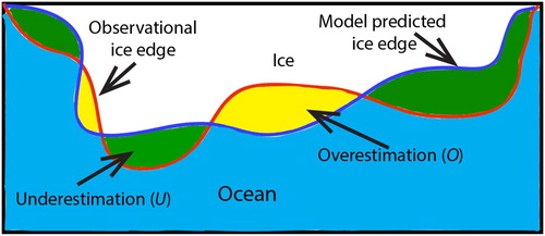
We investigated the accuracy of IcePOM’s 10-day sea ice forecast in the Chukchi Sea area. Since MIRAI needs to avoid sea ice as much as possible, ice edge error and bias were used to quantify forecast skill. Goessling, Tietsche, Day, Hawkins, and Jung (2016) introduced ice edge error – average distance between forecast and observed ice edges – and bias estimation methods, which were subsequently recommended by Melsom, Palerme, and Müller (2019). Figure 3 shows the schematic diagram of predicted (blue) and observational (red) ice edges. Yellow areas indicate model overestimation (O), which is the spatial integral of all sea ice extents where predicted ice concentration is above 15% but observed sea ice concentration is below 15%. Green areas indicate model underestimation (U), which is the spatial integral of all sea ice extents where predicted ice concentration is below 15% but observed ice concentration is above 15%. Light blue and white areas indicate ocean extent that has been correctly predicted and sea ice extent that has been correctly predicted, respectively. Ice edge error and bias are defined in Equations (1) and (2), respectively:

Figure 3. Schematic diagram of predicted (blue) and observational (red) ice edges. Yellow areas indicate model overestimation (O), which is the spatial integral of all sea ice extents where predicted ice concentration is above 15% but observed ice concentration is below 15%. Green areas indicate model underestimation (U), which is the spatial integral of all sea ice extents where predicted ice concentration is below 15% but observed ice concentration is above 15%. Light blue and white areas indicate ocean extent that has been correctly predicted and sea ice extent that has been correctly predicted, respectively.

(1) $\mathrm{I}\mathrm{c}\mathrm{e}\mathrm{e}\mathrm{d}\mathrm{g}\mathrm{e}\mathrm{e}\mathrm{r}\mathrm{r}\mathrm{o}\mathrm{r}=\frac{O+U}{\left(1/2\right)\left(L_m+L_o\right)}$(1) (2) $\mathrm{B}\mathrm{i}\mathrm{a}\mathrm{s}=\frac{O-U}{\left(1/2\right)\left(L_m+L_o\right)}$(2) where L_m and L_o are the length of predicted ice edge and length of observational ice edge, respectively.

During the melting and freezing months, melt ponds, moist snow and wet ice surface negatively bias AMSR2 sea ice concentration and ice edge location. In addition, effective resolution of the AMSR2 sea ice concentration product is about 10 km, which is lower than the resolution of the model grid. Biases in AMSR2 data and the relative coarseness of AMSR2 data can introduce uncertainties into the estimates of ice edge error.

Forecast skill is indicated by ice edge error, bias and sea ice concentration distribution with respect to AMSR2 data and Interactive Multisensor Snow and Ice Mapping System (IMS; Helfrich, McNamara, Ramsay, Baldwin, & Kasheta, 2007) ice mask product. The IMS product has a resolution of 1 km; sea ice is indicated where sea ice concentration is greater than 40%; open water is indicated where sea ice concentration is less than 40%. Therefore when calculating ice edge error with respect to IMS data, ice edge is defined as where sea ice concentration is 40%. Skill scores are computed for 10-day forecasts initialized between 1 and 25 November 2018. Skill score results are presented in Section 3.

3. Results

To navigate safely, MIRAI requests forecasts of sea ice and ocean variables every day; these include distributions of sea ice concentration, thickness and pressure, ice edge location defined by thresholds of 5% and 15% ice concentrations, and sea surface temperature distribution. It takes IcePOM about 55 min to compute variables for one simulated day. Every day, IcePOM downloads AMSR2 sea ice concentration and thickness data at 05:00 UTC and ECMWF atmospheric forecast data at 05:45 UTC from the ADS server. After interpolating AMSR2 and ECMWF data on to the model grid, IcePOM starts the forecast computation at 06:30 UTC. Forecast of the first of ten days is uploaded on to the ADS server at 07:45 UTC and forecast of the tenth day is uploaded at 14:45 UTC.

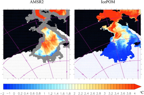
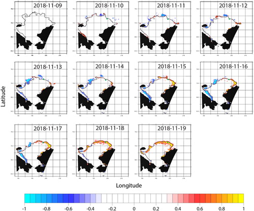
Figure 4 shows evolution of the difference between predicted and AMSR2 observational sea ice concentration distributions; model run was initiated on 9 November 2018 and forecasts were made for 9–19 November 2018. Black contour indicates AMSR2 observational ice edge location (15% concentration threshold). Green dots indicate locations of the ice edge observed from MIRAI and aerial photos taken from the same locations are shown in Figure 5. Difference between model and AMSR2 sea ice concentrations is greater than ±30%. On 12 November (third day of forecast) the model starts to overestimate sea ice; to the north of Alaska, ice continues to grow, creating further errors in the advance of the ice edge. We examined possible factors underlying the large difference between model and satellite sea ice concentrations and found that sea surface temperature (SST) in IcePOM is lower than that from AMSR2; SST distribution in the Chukchi Sea in IcePOM is also different from that from AMSR2 (Figure 6). North of 70 °N, SST in IcePOM is about 4°C lower than that from AMSR2.

Figure 4. Evolution of difference between predicted and Advanced Microwave Scanning Radiometer 2 (AMSR2) observational sea ice concentration distributions for 9–19 November 2018. Model run starts from 9 November 2018. Black contour indicates AMSR2 ice edge (15% concentration threshold). Green dots indicate locations of ice edge observed from MIRAI. Aerial photos taken from the same locations are shown in Figure 5.

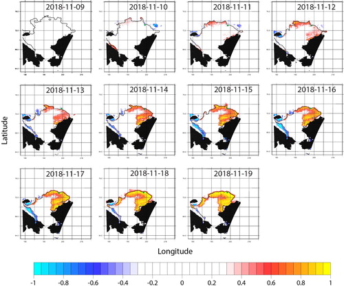
Figure 5. Sea ice conditions at the conductivity, temperature and depth (CTD) observation stations in the marginal ice zone for 10–19 November 2018. Photographs were taken between 2000 and 2300 UTC. (The original date is shown in the right bottom corner of each photograph).

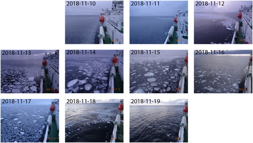
Figure 6. Sea surface temperature distribution on 9 November 2018 (left: AMSR2, right: IcePOM). White areas indicate presence of sea ice and gray areas indicate missing data.

We considered two hypotheses to explain the low SSTs in the Chukchi Sea area in IcePOM. First, warm and fresh water input into the Bering Strait is underestimated because of the climatological values restored from the Bering strait boundary to the south of the domain. Second, heat input into sea ice and ocean is underestimated by the bulk formulation used in the model. Impact of the first hypothesis is likely to be dominant; therefore, we tested the first hypothesis by replacing output from the pan-Arctic model with output from the Canadian Regional Ice Ocean Prediction System (RIOPS) as initial and boundary conditions. We conducted a hindcast for 1 October to 1 November 2018 using RIOPS temperature and salinity [http://dd.alpha.meteo.gc.ca/yopp/model_riops/] as initial and boundary conditions at the Bering Strait for the high-resolution regional model (Figure 2(b)).

We chose RIOPS because it includes a full multivariate ocean data assimilation system that combines satellite observations of sea level anomaly and SST together with in situ observations of temperature and salinity. In situ observations are obtained from a variety of sources, including the Argo network of autonomous profiling floats, moorings, ships, marine mammals and research cruises.

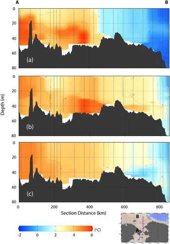
Modeled ocean structure was improved by RIOPS boundary conditions. Figure 7 shows vertical temperature profiles along a cross section between the Bering Strait (66 °N, 168.75 °W) and the Chukchi Sea (73 °N, 186.75 °W) for 7 November 2018. It shows profiles based on IcePOM forecast with climatological boundary conditions, CTD observations from MIRAI, and IcePOM forecast with RIOPS boundary conditions at the Bering Strait. It is clear that IcePOM forecast with RIOPS boundary conditions adequately reproduces MIRAI observations, including weak stratification throughout the entire water column in the Chukchi Sea (located at 400–850 km in the section in Figure 7). Intrusion of warm and fresh Pacific water into the Chukchi Sea is clearer in IcePOM forecast after boundary conditions have been corrected with RIOPS (Figure 7).

Figure 7. Vertical profiles of ocean temperature on 7 November 2018 along section A–B of cruise track indicated in Figure 1. (a) IcePOM forecast with climatological boundary conditions, (b) conductivity, temperature and depth observations from the research vessel MIRAI, and (c) IcePOM forecast with RIOPS boundary conditions.

Similar to Figure 4, Figure 8 shows the difference between predicted and AMSR2 observational sea ice concentration distributions from 9 to 19 November 2018 but model output is obtained with RIOPS boundary conditions. A qualitative comparison of Figures 4 and 8 shows that RIOPS boundary conditions greatly reduce overestimation of sea ice to the north of Alaska, suggesting that assimilation of observational SST data into the model might further improve the model’s forecasts.

Figure 8. Same as Figure 4 but model is run with RIOPS boundary conditions.

Figure 9 shows ice edge errors and biases of sea ice forecasts from various models for 1–25 November 2018. Errors and biases were calculated with respect to AMSR2 (Figure 9(a,b)) and IMS data (Figure 9(c,d)). Ice edge was defined by thresholds of 15% and 40% ice concentrations for comparison with AMSR2 and IMS, respectively. The following forecasts were analyzed: IcePOM 10-day forecast with RIOPS boundary conditions, IcePOM 10-day forecast with climatological boundary conditions, TOPAZ4 forecast, ECMWF 10-day forecast and persistence of the AMSR2 and IMS observations.

Figure 9. Evolution of ice edge errors and bias for 1–25 November 2018 from IcePOM 10-day forecast with RIOPS boundary conditions, IcePOM 10-day forecast with climatological boundary conditions, TOPAZ4 forecast, ECMWF 10-day forecast and persistence of the observations. Errors and biases were calculated with respect to Advanced Microwave Scanning Radiometer 2 (AMSR2) ((a) and (b)) and Interactive Multisensor Snow and Ice Mapping System (IMS) data ((c) and (d)). Ice edge was defined by thresholds of 15% and 40% ice concentrations for comparison with AMSR2 and IMS, respectively.

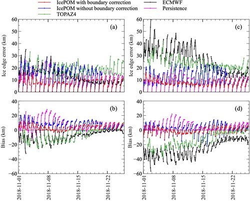
For IcePOM forecast with climatological boundary conditions, maximum ice edge errors with respect to AMSR2 and IMS are 29 and 25 km, respectively. For IcePOM forecast with RIOPS boundary conditions, maximum ice edge errors with respect to AMSR2 and IMS are reduced to 16 and 17 km, respectively. RIOPS model with 2-day forecast, maximum ice edge error is 14 km during this period (not shows in Figure 9). For ECMWF and TOPAZ4 forecasts, maximum ice edge errors with respect to AMSR2 are 35 and 33 km, and maximum ice edge errors with respect to IMS are 60 and 42 km. Ice edge forecasts of IcePOM are comparable to those of the other models. After 15 November, ice edge error from TOPAZ4 and ECMWF decrease, with the TOPAZ4 errors reaching levels of the same magnitude as that from IcePOM. Figure 9(a) shows that initial ice edge error of IcePOM with respect to AMSR2 has a value of zero. This is because IcePOM is initialized with sea ice concentration derived from AMSR2 while ECMWF and TOPAZ4 models assimilate the Operational Sea Surface Temperature and Ice Analysis (OSTIA) system products.

With respect to both AMSR2 and IMS, ice edge forecasts from ECMWF and TOPAZ4 are negatively biased, while those of IcePOM are positively biased (Figure 9(b,d)). The negative bias of ECMWF forecasts reduces with time.

Figure 10 shows evolution of IcePOM overestimation and underestimation of sea ice extent for 9–19 November 2018 (same period in Figures 4 and 8). Compared with AMSR2 observations, IcePOM underestimates sea ice extent between 9 and 14 November, and overestimates it after 14 November. To further understand model bias, we plotted time–depth cross sections of ocean temperature (Figure 11) and salinity (Figure 12) at the MIZ for 10–20 November 2018. Data sources include CTD observations from MIRAI (Figures 11(a) and 12(a)), initial field from RIOPS forecast (Figures 11(b) and 12(b)), initial field from IcePOM forecast with RIOPS boundary conditions (Figures 11(c) and 12(c)), and initial field from IcePOM forecast with climatological boundary conditions (Figures 11(d) and 12(d)). Locations of CTD observations are shown in Figures 11(e) and 12(e). IcePOM forecast with climatological boundary shows that sea ice forms quickly near the MIZ because of the presence of colder water (temperature was near freezing every day) and not because of the presence of fresher water. Variability of the upper mixed layer in IcePOM with RIOPS boundary conditions is of the same magnitude as that from MIRAI observations. Temporal variation of salinity in all models is lower than that in observations. However, neither IcePOM with RIOPS boundary conditions nor RIOPS reproduces the upwelling of warmer and saltier water to the upper 30 m of the water column on 19 and 20 November.

Figure 10. Evolution of IcePOM overestimation and underestimation of sea ice extent distribution for 9–19 November 2018. Forecast begins on 9 November 2018. Ice edge is indicated by a threshold ice concentration of 15%. Ice edge from Advanced Microwave Scanning Radiometer 2 (AMSR2) is shown in black contour. Color scheme is the same as that in Figure 3.

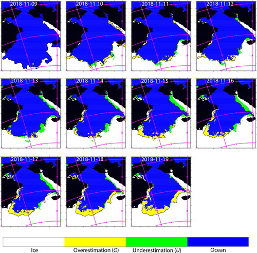
Figure 11. Time–depth cross section of ocean temperature for 10–20 November 2018 at the marginal ice zone. (a) results from conductivity, temperature and depth (CTD) observations from MIRAI, (b) RIOPS forecast, (c) IcePOM forecast with RIOPS boundary conditions, (d) IcePOM forecast with climatological boundary condition, and (e) locations of CTD observations.

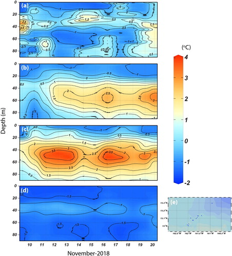
Figure 12. Time–depth cross section of ocean salinity for 10–20 November 2018 at the marginal ice zone. (a) results from conductivity, temperature and depth (CTD) observations from MIRAI, (b) RIOPS forecast, (c) IcePOM forecast with RIOPS boundary conditions, (d) IcePOM forecast with climatological boundary condition, and (e) locations of CTD observations.

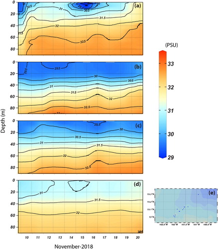
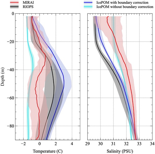
Figure 13 shows time-averaged temperature and salinity profiles at the MIZ with mean (thick lines) and standard deviation (shading). With respect to observations, IcePOM with RIOPS boundary conditions has a negative bias in salinity and a positive bias in temperature. Model forecasts differ from observations in a number of areas that are yet to be investigated. For example, IcePOM forecasts the presence of a warm water mass at depths of 40–70 m, which is absent in observations; water salinity in the upper layer in IcePOM is lower than that in observations; temporal variation of salinity in all models is lower than that in observations.

Figure 13. Time-averaged temperature and salinity profiles at the marginal ice zone for the data presented in Figures 10 and 11. Thick lines indicate average values and shading indicates standard deviation.

4. Concluding remarks

In this paper, we conducted a detailed analysis of the real-time sea ice forecasts created for the expedition of the RV MIRAI in November 2018. Maps indicating sea ice concentration, thickness and pressure and the location of the ice edge are important for operational planning of maritime activities. We also highlighted the importance of the ability of medium range sea ice forecasts to precisely reproduce SST and oceanic lateral boundary conditions. Our results suggest that IcePOM is capable of predicting the sea ice cover with a lead time of 10 days and a maximum ice edge error of less than 16 km if the adequate ocean boundary conditions are provided.

Acknowledgements

The authors wish to acknowledge support from the Green Network of Excellence Program – Arctic Climate Change Research Project (GRENE-Arctic) and Arctic Challenge for Sustainability Research Project (ArCS) by the Japanese Ministry of Education, Culture, Sports, Science and Technology and a Kakenhi grant (no. 26249133, 18H03745, 18KK0292) from the Japan Society for the Promotion of Science. Their gratitude is extended to Arctic Data Archive System for providing for the gridded AMSR-2 data and ECMF atmospheric forecast data and Regional Ice Ocean Prediction System (RIOPS) for the gridded ocean temperature and salinity data. This is a contribution to the Year of Polar Prediction (YOPP), a flagship activity of the Polar Prediction Project (PPP), initiated by the World Weather Research Programme (WWRP) of the World Meteorological Organisation (WMO).

Disclosure statement

No potential conflict of interest was reported by the authors.

Additional information

Funding

This work was supported by the Japan Society for the Promotion of Science under a Kakenhi grant (no. 26249133, 18H03745, 18KK0292).

References

- Buehner, M., Caya, A., Pogson, L., Carrieres, T., & Pestieau, P. (2013). A new environment Canada regional ice analysis system. Atmosphere-Ocean, 51, 18–34. doi: 10.1080/07055900.2012.747171
- Dee, D. P., Uppala, S. M., Simmons, A. J., Berrisford, P., Poli, P., Kobayashi, S., … Vitart, F. (2011). The ERA-Interim reanalysis: Configuration and performance of the data assimilation system. Quarterly Journal of the Royal Meteorological Society, 137, 553–597. doi: 10.1002/qj.828
- De Silva, L. W. A., & Yamaguchi, H. (2017). The impact of data assimilation and atmospheric forcing data on predicting short-term sea ice distribution along the Northern sea route. Okhotsk Sea Polar Oceans Research, 1, 1–6.
- De Silva, L. W. A., Yamaguchi, H., & Ono, J. (2015). Ice–ocean coupled computations for sea-ice prediction to support ice navigation in Arctic sea routes. Polar Research, 34, 18p. doi: 10.3402/polar.v34.25008
- Fujisaki, A., Yamaguchi, H., & Mitsudera, H. (2010). Numerical experiments of air–ice drag coefficient and its impact on ice–ocean coupled system in the Sea of Okhotsk. Ocean Dynamics, 60, 377–394. doi: 10.1007/s10236-010-0265-7
- Goessling, H. F., Tietsche, S., Day, J. J., Hawkins, E., & Jung, T. (2016). Predictability of the Arctic sea ice edge. Geophysical Research Letters, 43, 1642–1650. doi: 10.1002/2015GL067232
- Hebert, D. A., Allard, R. A., Metzger, E. J., Posey, P. G., Preller, R. H., Wallcraft, A. J., … Smedstad, O. M. (2015). Short-term sea ice forecasting: An assessment of ice concentration and ice drift forecasts using the U.S. Navy’s Arctic Cap Nowcast/forecast system. Journal of Geophysical Research: Oceans, 120, 8327–8345. doi: 10.1002/2015JC011283
- Helfrich, S. R., McNamara, D., Ramsay, B. H., Baldwin, T., & Kasheta, T. (2007). Enhancements to, and forthcoming developments in the interactive multisensor snow and ice mapping system (IMS). Hydrological Processes, 21, 1576–1586. doi: 10.1002/hyp.6720
- Hunke, E. C., & Dukowicz, J. K. (2002). The elastic–viscous–plastic sea ice dynamics model in general orthogonal curvilinear coordinates on a sphere—incorporation of metric terms. Monthly Weather Review, 130, 1848–1865. doi: 10.1175/1520-0493(2002)130<1848:TEVPSI>2.0.CO;2
- Inoue, J., Yamazaki, A., Ono, J., Dethloff, K., Maturilli, M., Neuber, R., … Yamaguchi, H. (2015). Additional Arctic observations improve weather and sea-ice forecasts for the Northern Sea Route. Scientific Reports, 5, 16868. doi: 10.1038/srep16868
- Krishfield, R. A., Proshutinsky, A., Tateyama, K., Williams, W. J., Carmack, E. C., McLaughlin, F. A., & Timmermans, M.-L. (2014). Deterioration of perennial sea ice in the Beaufort Gyre from 2003 to 2012 and its impact on the oceanic freshwater cycle. Journal of Geophysical Research: Oceans, 119, 1271–1305. doi: 10.1002/2013JC008999
- Kubat, I., Sayed, M., Savage, S. B., & Carrieres, T. (2010). Numerical simulations of ice thickness redistribution in the Gulf of St. Lawrence. Cold Regions Science and Technology, 60, 15–28. doi: 10.1016/J.COLDREGIONS.2009.07.003
- Mellor, G. L., Hakkinen, S., Ezer, T., & Patchen, R. (2002). A generalization of a sigma coordinate ocean model and an intercomparison of model vertical grids. In In ocean forecasting: Conceptual basis and applications (pp. 55–72). Berlin Heidelberg: Springer.
- Mellor, G. L., & Yamada, T. (1982). Development of a turbulence closure model for geophysical fluid problems. Reviews of Geophysics, 20, 851–875. doi: 10.1029/RG020i004p00851
- Melsom, A., Palerme, C., & Müller, M. (2019). Validation metrics for ice edge position forecasts. Ocean Science, 15, 615–630. doi: 10.5194/os-15-615-2019
- Mudunkotuwa, D. Y., De Silva, L. W. A., & Yamaguchi, H. (2016). Data assimilation system to improve sea ice predictions in the Arctic ocean using an ice-ocean coupled model. Proceedings of the 23rd IAHR international symposium on ice (pp. 1–8), Ann Arbor, MI.
- Nakanowatari, T., Inoue, J., Sato, K., Bertino, L., Xie, J., Matsueda, M., … Otsuka, N. (2018). Medium-range predictability of early summer sea ice thickness distribution in the East Siberian Sea based on the TOPAZ4 ice–ocean data assimilation system. The Cryosphere, 12, 2005–2020. doi: 10.5194/tc-12-2005-2018
- Ono, J., Inoue, J., Yamazaki, A., Dethloff, K., & Yamaguchi, H. (2016). The impact of radiosonde data on forecasting sea-ice distribution along the Northern Sea Route during an extremely developed cyclone. Journal of Advances in Modeling Earth Systems, 8, 292–303. doi: 10.1002/2015MS000552
- Parkinson, C. L., & Washington, W. M. (1979). A large-scale numerical model of sea ice. Journal of Geophysical Research, 84, 311–337. doi: 10.1029/JC084iC01p00311
- Preller, R. H., & Posey, P. G. (1989). The Polar ice prediction system – a sea ice forecasting system, Naval Ocean Research and Development Activity Rep. 212. Mississippi.
- Sagawa, G., & Yamaguchi, H. (2006). A semi-lagrangian sea ice model for high resolution simulation. In The sixteenth international offshore and polar engineering conference (pp. 584–590). San Francisco, CA: International Society of Offshore and Polar Engineers.
- Sakov, P., Counillon, F., Bertino, L., Lisæter, K. A., Oke, P. R., & Korablev, A. (2012). TOPAZ4: An ocean-sea ice data assimilation system for the North Atlantic and Arctic. Ocean Science, 8, 633–656. doi: 10.5194/os-8-633-2012
- Schweiger, A. J., & Zhang, J. (2015). Accuracy of short-term sea ice drift forecasts using a coupled ice-ocean model. Journal of Geophysical Research: Oceans, 120, 7827–7841. doi: 10.1002/2015JC011273
- Semtner, A. J. (1976). A model for the thermodynamic growth of sea ice in numerical investigations of climate. Journal of Physical Oceanography, 6, 379–389. doi:10.1175/1520-0485(1976)006<0379:AMFTTG>2.0.CO;2
- Smagorinsky, J. (1963). General circulation experiments with the primitive equations. Monthly Weather Review, 91, 99–164. doi:10.1175/1520-0493(1963)091<0099:GCEWTP>2.3.CO;2
- Steele, M., Morley, R., & Ermold, W. (2001). PHC: A global ocean hydrography with a high-quality Arctic ocean. Journal of Climate, 14, 2079–2087. doi:10.1175/1520-0442(2001)014<2079:PAGOHW>2.0.CO;2
- Turnbull, I. D., & Taylor, R. S. (2017). An operational thermodynamic-dynamic model for the coastal Labrador Sea ice melt season. Geoscientific Model Development Discussions, 2017, 1–57. doi: 10.5194/gmd-2017-39
- Zhang, X., & Zhang, J. (2001). Heat and freshwater budgets and pathways in the Arctic Mediterranean in a coupled ocean/sea-ice model. Journal of Oceanography, 57, 207–234. doi: 10.1023/A:1011147309004