Grinding optimization using nondestructive testing (NDT) and empirical models

Abstract

Proper choice of grinding parameters is important because productivity is limited by the possibility of grinding burns. Nondestructive testing (NDT), as Barkhausen noise (BN), can provide a tool for determining parameter limits. However, BN requires a threshold value for approval and requires multiple experiments to provide grinding parameters corresponding to high productivity. Other limiting process outputs, such as surface roughness, need to be fulfilled. In this study, process modeling, experiments and NDT are combined to produce optimized grinding parameters that fulfill the process output requirements and reduces the number of experiments for a new component. Design of experiments (DOE) grinding tests were performed with cutting power measurements. The outcome was verified with BN and surface roughness outputs. Then, using polynomial fitting, regression models were fitted into the BN, surface roughness and cutting power data. Malkin’s temperature model was utilized to analyze the temperature rise in the grinding zone. Combining all models, a grinding productivity optimization problem was defined from a specific material removal rate perspective. The polynomial fits of BN results and cutting power showed good prediction capability, as expressed by their R² values. The study provides a novel method to choose grinding parameters to produce quality parts with minimal loss of productivity.

Keywords:

• Barkhausen noise
• grinding
• modeling
• quality control
• residual stress

Introduction

Grinding is a common method to acquire the final surface integrity, shape and correct specified manufacturing tolerances. It is a suitable method for hardened components with demanding profiles, such as different gears for example. As Karpuschewski and Inasaki (2006) concluded, the grinding process is highly dependent on the tool's (grinding wheel) performance, selection and conditioning. Additionally, a poor choice of grinding parameters leads to increased heat input into the workpiece. This might compromise the workpiece's surface integrity and cause surface damages called grinding burns. As Malkin and Guo (2007) stated, most grinding damage is thermal in origin. The temperature rise may either cause rehardening burns with a moderate temperature increase, rehardening burns with phase transformation at higher temperatures or unfavorable tensile residual stresses (Malkin and Guo, 2007). However, the outcome of the residual stresses is complex and is caused by the effects of mechanical deformation, thermal expansion and contraction and material phase transformation during the grinding (Chen et al., 2000). The surface integrity layer quality (optimal surface roughness, no grinding burns, adequate manufacturing tolerances, etc.) will highly depend on the correct parameters utilized in the grinding. One common post-process online quality control method for detecting unwanted changes caused by grinding is the magnetic nondestructive Barkhausen noise (BN) method. Grinding burn detection is the most common industrial application of this method. BN is sensitive to changes in the microstructural state and residual stresses as they affect the magnetic domain motion, which creates the measurable BN emissions. Therefore, these changes show the existence of heat-affected areas, as they have variations in microstructure and stress state compared to the surrounding material. Usually, the online quality control judges the BN outcome with the “pass-no pass method” compared to a certain reference level that has been accepted and verified with other means earlier.

Grinding is often used as a finishing process. Mistakes made that late in the total manufacturing process are costly, as resources allocated up to that point to manufacture the component are lost. As most of the challenges in grinding are caused by too high heat input (Malkin and Guo, 2007) and as the direct measurement of contact surface temperature between the grinding wheel and the ground surface is difficult, some other methods have been utilized for the determination of grinding temperature thresholds for grinding burns. Thanedar et al. (2019) studied the cylindrical grinding process and used an analytical model to determine the grinding temperature and correlate it with the occurrence of grinding burns. The model was validated experimentally with Barkhausen noise measurements. For the cylindrical grinding process, they noticed a threshold temperature of 631 °C in the grinding zone, after which grinding burns were observed with the hardened micro-alloyed steel. Thanedar et al. (2019) found that all the varied grinding parameters (low-high levels): work speed, wheel speed, in feed, coolant flow, dressing in-feed and spark out time influenced the measured BN response. Increasing work speed was noticed to decrease the measured BN response due to decreased heat generation within the interaction zone. Whereas increasing the depth of cut or decreasing the coolant flow increases the BN response. As an optimal point that provides the optimal grinding parameters, they (Thanedar et al., 2019) concluded; wheel speed 90 m/s, work speed 90 m/s, spark out time 15 s and in-feed 0.09 mm/min. Karpuschewski et al. (2011) noticed that increasing the material removal rate Q_w would cause the inspected Barkhausen noise signal to increase. In addition, increasing either the wheel speed or the work speed was noticed (Thanedar et al., 2019) to decrease the BN signal by decreasing the heat generation in the interaction zone. Whereas the increase in depth of cut (in-feed mm/min) and lower-level coolant flow has also led to a dramatic increase in BN signal (Thanedar et al., 2019).

One important parameter in grinding is the grinding wheel topography which is controlled by dressing the grinding wheel periodically by a diamond dresser with a certain axial speed and depth of cut. The effect of dressing has been investigated, that is, in Thanedar et al. (2019) and in Liu et al. (2017). Liu et al. (2017) noticed that in grinding tangential forces increased dramatically, as the dressing overlap ratio (U_d) increased (finer wheels and more contact points to the surface may cause heat generation). Thanedar et al. (2019) noticed that higher dressing in-feed produced lower levels of BN. Micietova et al. (2017) studied the BN envelopes of grinding burns, and the main variable in grinding was the gradual grinding wheel wear as the wheel was not redressed while grinding the samples. This increases friction, and therefore, heat generation between the grinding wheel and the workpiece surface. They noticed a gradual increase in BN to a certain level of wheel wear, after which re-hardening burn occurred and BN was decreased. Also, Azarhoushang et al. (2017) studied the effect of external cylindrical grinding to the produced residual stresses and Barkhausen noise output after dry grinding. They compared the required grinding force and grinding temperature of a structured grinding wheel to a non-structured grinding wheel. Before structuring, both wheels were dressed using the same dressing overlap-ratio (U_d), speed ratio and depth of dressing. As the ground components were characterized with surface residual stress measurements, they noticed that too high a specific material removal rate Q’_w and too high dressing overlap ratio would produce undesired tensile residual stresses even in wet grinding conditions. They also noticed that higher surface residual stresses were induced on larger diameter workpieces due to the larger contact length. The BN results were in normal trend compared to surface residual stresses; higher tensile stress produced higher BN response. They concluded that by using a 75% structured wheel, the thermal damages can be reduced.

Usually, the Barkhausen noise-based systems are utilized in post-process grinding burn inspection. Some recent publications have utilized BN-based measurement systems for in-process monitoring purposes in real time inside the grinding machine (Jedamski et al., 2020). This novel type of analysis would bring together the benefits of BN measurements for surface integrity studies and save time in production. In addition, novel modeling approaches have been studied, that is, Heinzel et al. (2019) combined Malkin’s grinding burn limit, thermal modeling and experimental grinding studies to determine the critical residual stress state on the surface via the Barkhausen noise measurements.

Although Barkhausen noise measurement has an established position in the industry for grinding burn detection (Karpuschewski et al., 2020), the amount of research on how the grinding parameters affect the BN signal is limited. Also, the research has been focusing on grinding burn detection. Hence, additional studies are needed to further the knowledge on how different grinding parameters affect the BN signal and how this information can be used to maximize productivity. For a new component, the grinding process parameters are not known, requiring costly experiments. In this study, grinding experiments, modeling and nondestructive testing using Barkhausen noise is combined to optimize grinding parameters to achieve the desired outcome: suitable surface roughness without grinding burns. At first to this new component for grinding, grinding experiments based on the design of experiments (DOE) were carried out. After the grinding, BN measurements were carried out to verify the outcome of the grinding process, for example to reveal possible grinding burns. The main research objective of this work is to analyze the effect of grinding parameters on the surface integrity of the ground workpieces with a focus on the induced residual stresses and surface roughness. The work presents a novel approach incorporating experimental measurements, data-based models and analytical models for productivity optimization in external cylindrical grinding.

Materials and methods

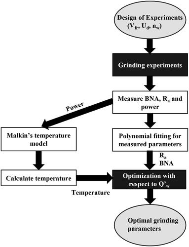
The flowchart illustrated in Figure 1 represents the structure of this study. At first, based on a design of experiments, grinding experiments were carried out. Different material characterization methods were applied to the ground components to provide data for polynomial fits. Then Malkin’s temperature model was utilized to analyze the temperature rise in the grinding zone. Utilizing the polynomial fits and the temperature model, a grinding productivity optimization problem was defined. This was done from the specific material removal rate perspective to select optimal grinding parameters for minimum temperature.

Figure 1. A flowchart describing the structure of this study.

The ground samples were cylindrical steel bars with a diameter of 29 mm manufactured from commercial low-alloyed tool steel AISI/SAE L6, which were through-hardened. The grinding experiments were performed with the S41 (Fritz Studer AG) external cylindrical grinding machine at Werkzeugmaschinenlabor WZL RWTH Aachen University (Germany). Quakercool coolant 3618 HBFF was used, and the coolant flow was kept constant. Aluminum oxide grinding wheel 32A60JVBE (500 × 35 x 203,2 mm) (NORTON) with vitrified bond with a medium grain size (60) was utilized. Dressing of the grinding wheel was done with a dressing-plate (Saint-Gobain). The wheel was dressed before each grinding step: rough plunge grinding, finishing plunge grinding and polishing. The dressing overlap ratio was controlled by measuring the active width of the dressing tool, and the axial feed rate was set to acquire the required overlap ratio.

At first, grinding trials were made to define the reference values for the grinding parameters that produced decent outcome and caused no grinding burns. This was verified by comparing it to an earlier obtained threshold value for this specific material. After this, a design of experiment was done to set up the variables in the grinding. The samples were ground with a wide range of different grinding parameters to obtain changes in the BN response. The chosen grinding parameters were the workpiece circumferential speed (n_w), dressing overlap-ratio (U_d), and (radial) feed rate (v_fr). Each parameter was varied on three levels, and a total of 27 experiments were conducted. Three experiments were reserved for a study on how multiple grinding processes, that is, rough grinding and finish grinding, affect the final workpiece surface integrity. Other grinding parameters were kept constant, grinding wheel peripheral speed v_s (40 m/s), depth of cut 2 mm and coolant flow.

After each grinding experiment, the average RMS value of the BN was measured from the sample surface. Barkhausen noise measurements were taken using a Rollscan 300 BN analyzer manufactured by Stresstech Oy (Finland) using two different sensors. Measurements in the longitudinal direction were measured at Werkzeugmaschinenlabor WZL RWTH Aachen (Germany) using an S4560 sensor with a 5 Vpp (peak-to-peak voltage) measurement voltage and 125 Hz measurement frequency. An analyzing frequency range of 70–200 kHz was utilized.

For a smaller subset of the samples whose process parameters showed potential for expressing a wide range of process outcomes, measurements in tangential direction were carried out at Tampere University (Finland) with a commercial sensor S5857 manufactured by Stresstech (Finland) optimal for curved surfaces. The measurements were taken with a magnetizing frequency of 125 Hz and magnetizing voltage of 8 Vpp. Microscan software was used to record the raw BN data. The BN method is suitable for grinding burn detection due to the variable analyzing frequency; in these studies, the maximum measurement depth was approximately between 150 µm−20 µm depending on the analyzing frequency range of 20–1000 kHz (Moorthy et al., 2003).

The samples were first screened for changes in the RMS level. Then, two different measurement lines were determined. RMS outputs were recorded in fixed measurement locations along these lines.

Surface roughness measurements were carried out with the MarSurf M 300 Mahr surface roughness device to measure the arithmetic mean roughness (Ra) of the surface. Cutting power was recorded as spindle power by the Vacon frequency converter. Residual stresses in both the longitudinal and tangential directions of the workpiece surface were measured from a subset of the ground workpieces. These measurements were done for the same subset of samples whose tangential average RMS value of the BN was measured. The subset was chosen such that the samples within the subset would still show the effects of each grinding parameter on the residual stresses. The surface residual stress (RS) and full width at half maximum (FWHM) of the diffraction peak values were examined. The measurements were taken from the same locations as in the BN measurement using an XStress 3000 X-ray diffractometer (XRD), manufactured by Stresstech Oy (Finland). The surface RS measurements were taken using CrKa radiation and the modified Chi-squared method (SFS-EN 15305, 2008). The measurement current and voltage were 6.7 mA and 30 kV, respectively. The residual stress measurement method with X-ray diffraction gives information about 5–6 µm depth below the surface with the used Cr-radiation (Hauk, 1997). The XRD residual stress measures type I (macro-) and II (micro-) stresses where the length scale is from grains to a large quantity of grains. Type III stress affects the full width at half maximum (FWHM) of the diffraction peak as it is influenced by dislocations, for example (Schajer, 2013). Residual stress depth measurements were done by the step-by-step electrolytic removal of thin layers with Movipol-3 electrolytic polishing equipment (Struers, Ballerup, Denmark) and Struers A2 perchloric acid solution. The depth of the removed layer was verified using a Mitutoyo dial indicator.

Based on the experimental study, a second-order polynomials were fitted to the experimental data. These models describe the behavior of the average root mean square (RMS) value of the BN, referred to as BNA hereinafter, surface roughness (Ra), and cutting power (P_c) as functions of the grinding parameters. The cutting power model was used to compute the maximum grinding temperature based on Malkin’s temperature model. By defining limits for BNA, surface roughness, and cutting power, an optimal parameter combination with respect to grinding productivity can be found using these polynomial models.

Design of experiments and polynomial fitting

A second-order polynomial models were fitted to the measured data of the RMS value of the BN, average mean surface roughness (Ra) and the cutting power (P_c) based on the design of experiments given in Table 1.

Table 1. Process parameter variables and their levels utilized in the design of experiment and models.

Process parameter	Variable	Level
		1	2	3
Radial feed rate	vfr (mm/min)	1.5	1.88	2.25
Dressing overlap ratio	Ud (-)	6	8.6	11.2
Workpiece circumferential speed	nw (1/min)	70	100	130

The first two models consider second-order interaction terms, while the last model considers only first-order interaction terms due to the lack of measurement data. A general second-order polynomial fit used in this study is given in equation 1(1) $$y=a_0+a_1{v}_{\mathit{\text{fr}}}+a_2{U}_d+a_3{n}_w+a_4{v}_{\mathit{\text{fr}}}{U}_d+a_5{v}_{\mathit{\text{fr}}}{n}_w+a_6{U}_d{n}_w+a_7{v}_{\mathit{\text{fr}}}{U}_d{n}_w+a_8{v}_{\mathit{\text{fr}}}^2+a_9{U}_d^2+a_{10}{n}_w^2+a_{11}{v}_{\mathit{\text{fr}}}^2{U}_d+a_{12}{\mathrm{v}}_{\mathit{\text{fr}}}^2{n}_w+a_{13}{U}_d^2{v}_{\mathit{\text{fr}}}+a_{14}{U}_d^2{n}_w+a_{15}{n}_w^2{v}_{\mathit{\text{fr}}}+a_{16}{n}_w^2{U}_d+a_{17}{v}_{\mathit{\text{fr}}}^2{U}_d^2+a_{18}{v}_{\mathit{\text{fr}}}^2{n}_w^2+a_{19}{U}_d^2{n}_w^2+a_{20}{v}_{\mathit{\text{fr}}}^2{U}_d^2{n}_w^2$$(1) , where y represents the estimation: (1) $$y=a_0+a_1{v}_{\mathit{\text{fr}}}+a_2{U}_d+a_3{n}_w+a_4{v}_{\mathit{\text{fr}}}{U}_d+a_5{v}_{\mathit{\text{fr}}}{n}_w+a_6{U}_d{n}_w+a_7{v}_{\mathit{\text{fr}}}{U}_d{n}_w+a_8{v}_{\mathit{\text{fr}}}^2+a_9{U}_d^2+a_{10}{n}_w^2+a_{11}{v}_{\mathit{\text{fr}}}^2{U}_d+a_{12}{\mathrm{v}}_{\mathit{\text{fr}}}^2{n}_w+a_{13}{U}_d^2{v}_{\mathit{\text{fr}}}+a_{14}{U}_d^2{n}_w+a_{15}{n}_w^2{v}_{\mathit{\text{fr}}}+a_{16}{n}_w^2{U}_d+a_{17}{v}_{\mathit{\text{fr}}}^2{U}_d^2+a_{18}{v}_{\mathit{\text{fr}}}^2{n}_w^2+a_{19}{U}_d^2{n}_w^2+a_{20}{v}_{\mathit{\text{fr}}}^2{U}_d^2{n}_w^2$$(1)

For the model fitted to cutting power data, coefficients a₁₁–a₂₀ were set to zero.

Malkin’s temperature model

According to Malkin and Guo (2008), the maximum temperature rise θ_m within the contact zone between a grinding wheel and a workpiece assuming a triangular heat source is (equation 2(2) $${\mathrm{\theta }}_m=\frac{1.06q_w{\mathrm{\alpha }}^{1/2}{l}_c^{1/2}}{k{v}_w^{1/2}}$$(2) ): (2) $${\mathrm{\theta }}_m=\frac{1.06q_w{\mathrm{\alpha }}^{1/2}{l}_c^{1/2}}{k{v}_w^{1/2}}$$(2)

Where q_w is the heat flux into the workpiece, α is the workpiece thermal diffusivity, l_c is the real contact length, k is the workpiece thermal conductivity, and v_w is the workpiece peripheral velocity, which is calculated from the workpiece circumferential speed: (3) $$v_w=\frac{n_w/60}{2\pi r\mathrm{ }}$$(3)

Where n_w is the workpiece circumferential speed and r is the workpiece radius.

The heat flux can be calculated from equation 4(4) $$q_w=\frac{\epsilon P_c}{l_c{b}_w}$$(4) (4) $$q_w=\frac{\epsilon P_c}{l_c{b}_w}$$(4) where ε is the heat partition ratio, P_c is the cutting power, b_w is the grinding wheel width, and l_c is the real contact length proposed by Rowe et al. (2013). It is based on the Hertz theory, assuming rough contact. The real contact length given in equation 5(5) $$l_c=\sqrt{\frac{8R_r^2{P}_c{d}_e}{\mathrm{\pi }{E}^{\mathrm{*}}\mathrm{\mu }{v}_s{b}_w}+a_e{d}_e}$$(5) (5) $$l_c=\sqrt{\frac{8R_r^2{P}_c{d}_e}{\mathrm{\pi }{E}^{\mathrm{*}}\mathrm{\mu }{v}_s{b}_w}+a_e{d}_e}$$(5) where v_s is the grinding wheel peripheral speed, µ is the cutting force ratio, d_e is the equivalent wheel diameter, a_e is the depth of cut, and E* is the combined elastic modulus of the grinding wheel and the workpiece given in equation 6(6) $$\frac{1}{E^{\mathrm{*}}}=\frac{1-{\nu }_1^2}{E_1}+\frac{1-{\nu }_2^2}{E_2}$$(6) (6) $$\frac{1}{E^{\mathrm{*}}}=\frac{1-{\nu }_1^2}{E_1}+\frac{1-{\nu }_2^2}{E_2}$$(6)

Where E is the elastic modulus and ν is the Poisson’s ratio, and index 1 refers to the workpiece and 2 to the wheel. For the roughness factor R_r, a typical value for wet grinding is 14 (Marinescu et al., 2013) which is used here.

In external cylindrical grinding, the equivalent wheel diameter is defined by equation 7(7) $$d_e=\frac{d_s{d}_w}{d_w+d_s}$$(7) : (7) $$d_e=\frac{d_s{d}_w}{d_w+d_s}$$(7) where d_s is the wheel diameter and d_w is the workpiece diameter. The depth of cut in external cylindrical grinding can be calculated from equation 8(8) $$a_e=\frac{v_{\mathit{\text{fr}}}}{n_w}$$(8) (8) $$a_e=\frac{v_{\mathit{\text{fr}}}}{n_w}$$(8) where v_fr is the feed rate and n_w is the workpiece circumferential speed. The process parameters for the temperature model are given in Table 2.

Table 2. Process parameters for the temperature model.

Process parameter	Explanation	Value (unit)
α	Workpiece thermal diffusivity	9.982e-6 (m^2/s)
ε	heat partition ratio	0.75 (-)
µ	Cutting force ratio	0.24 (-)
ρ	Workpiece density	7840 (kg/m^3)
bw	Grinding wheel width	35 (mm)
cp	Workpiece specific heat capacity	460 (J/(kgK))
ds	Grinding wheel diameter	500 (mm)
dw	Workpiece diameter	29 (mm)
E*	Combined elastic modulus	25.64 (GPa)
E1	Work modulus	213 (GPa)
E2	Wheel modulus	26 (GPa)
ν1	Work Poisson’s ratio	0.3 (-)
ν2	Wheel Poisson’s ratio	0.31 (-)
k	Workpiece thermal conductivity	36 (W/(mK))
Rr	Roughness factor	14 (-)
r	Workpiece radius	14.5 (mm)
vs	Grinding wheel peripheral speed	40 (m/s)

Productivity optimization

Specific material removal rate Q’_w can be used as a criterion to assess grinding productivity (Kopac and Krajnik, 2006). It is the volume of material removed from the workpiece per unit time and active grinding contact width, and is given in equation 9(9) $$Q_w^{\prime }=a_e{v}_w=\frac{v_{\mathit{\text{fr}}}}{n_w}{v}_w=\frac{v_{\mathit{\text{fr}}}}{60}{d}_w\pi$$(9) : (9) $$Q_w^{\prime }=a_e{v}_w=\frac{v_{\mathit{\text{fr}}}}{n_w}{v}_w=\frac{v_{\mathit{\text{fr}}}}{60}{d}_w\pi$$(9)

Maximizing the grinding productivity affects the considered process outcome parameters (BNA, temperature and workpiece surface roughness). Increasing the specific material removal rate increases the generated heat which increases temperature within the grinding contact zone. This can lead to grinding burn increasing BNA. In addition, workpiece surface roughness is affected by the grinding speed. Therefore, an optimization problem to maximize the specific material removal rate with respect of these three parameters was developed. The fitted polynomials of BNA, temperature and surface roughness are used in three inequality constraints. The limiting values (d_i) are 70 for BNA, 0.185 µm for surface roughness and 250 °C for temperature. The justification for these values is presented in later sections. In addition to inequality constraints, the process parameter values are limited by the design space defined in the design of experiments. After the optimization problem has been defined, the problem is solved using sequential least squared programming (SQLSP) (Kraft et al. 1994). The algorithm is such that it can only find a minimum. Therefore, the maximization is converted into minimization problem by searching the minimum of the negative value of the specific material removal rate.

The optimization problem has three inequality constraints (limiting values presented as d_i) and three lower and upper bounds on the grinding parameters. The problem is given as $$\mathrm{\text{min}}\mathrm{ }{-Q}_w^{\prime }$$ $$\mathit{\text{subject to}}:$$ $$\mathit{\text{Bn Average RMS}}\le d_1$$ $$R_a\le d_2$$ $${\mathrm{\theta }}_m\le d_3$$ $$1.5\le v_{\mathit{\text{fr}}}\le 2.25$$ $$6\le U_d\le 11.2$$ $$70\le n_w\le 130$$

The solution found by the SQLSP algorithm depends on the initial guess, that is, it finds a local optimum. Therefore, to find all the possible solutions, the algorithm was run using multiple different points within the space defined by the boundaries as initial guesses. Then all found solutions were compared with each other to find the global optimum.

Results

Experimental measurements

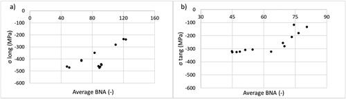
Usually, BNA and XRD residual stress have some relationship with each other’s (i.e., Stewart et al., 2004). Therefore, the relationship was determined also to these samples. The residual stresses were measured from the surface of the ground parts which belonged to a smaller subset of the whole experiment set. As seen in Figure 2, grinding produces much higher compressive residual stresses to the longitudinal direction of the studied cylindrical samples. Figure 2a presents the longitudinal residual stress that is given as a function of the RMS measured in RWTH Aachen in the longitudinal direction. This longitudinal measurement direction holds linear correlation between the surface residual stress and BNA, but there exist a group with quite high BNA values at about 90, for which the residual stresses remain low at about −450 MPa. It is not clear if this group of outliers is related to the actual grinding process or measurement process, as the parameters vary within the group. Whereas for the tangential residual stresses measured at Tampere university, in Figure 2b show linear relationship with the BNA values only at certain range of the stresses. For the larger compressive residual stresses (-320 MPa) in tangential direction, the BNA values are varying somewhat. As different BN equipment, BN sensors and different measurement parameters were used for BNA measurement in different measurement directions, the BNA scale is different in Figure 2a and 2b. Therefore, BNA values cannot be directly compared and in addition, the BN sensor properties might affect the sensor sensitivity properties as well.

Figure 2. Longitudinal (a) and tangential (a) residual stresses as a function of BNA.

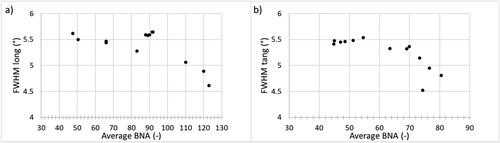
The full width half maximum (FWHM) of the XRD profiles was measured to have some estimation of the surface hardness states. In Figure 3a and 3b, XRD FWHM is shown as a function of BNA for different measurement directions. Similar separate group of measurement outliers (Figure 3a) is seen in these FWHM values as in longitudinal residual stresses (Figure 2a). FWHM in the tangential direction (Figure 3b) shows a plateau similar to that with residual stress but decreases as the value of BNA increases. Similar behavior is seen also in the longitudinal direction (Figure 3a). XRD FWHM is related to the hardness of the material, and this decreasing trend in FWHM with increasing BNA is typical.

Figure 3. Longitudinal (a) and tangential (a) XRD FWHM as a function of BNA.

Analysis of variance

In this article, analysis of variance (ANOVA) is applied to study the interactions between the grinding parameters. The three polynomial models were analyzed using ANOVA to find statistically significant terms (P-value less than 0.05). Table 3 shows the results of these analyses.

Table 3. ANOVA results.

Term	BNA	Surface roughness	Cutting power
	(R^2 = 99.2%)	(R^2 = 73.8%)	(R^2 = 98.3%)
Linear
vfr	S	S	S
Ud	I	I	S
nw	S	S	S
Square
vfr^2	S	I	I
Ud^2	S	I	I
nw^2	S	S	I
Interaction
vfrUd	S	S	S
vfrnw	S	I	S
Udnw	I	S	S
vfrUdnw	I	I	S
vfr^2Ud	S	I	–
vfr^2nw	S	I	–
Ud^2vfr	I	S	–
Ud^2nw	I	S	–
nw^2vfr	S	I	–
nw^2Ud	I	S	–
vfr^2Ud^2	S	I	–
vfr^2nw^2	S	I	–
Ud^2nw^2	I	S	–
vfr^2Ud^2nw^2	I	I	–

S: significant; I: Insignificant.

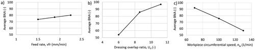
In both the BNA and surface roughness models, the linear term of the dressing overlap ratio (U_d) is insignificant. Whereas, in the cutting power model the linear term appears, which is an expected result. According to Liu et al. (2017), the tangential force increases as U_d increases. The same behavior was seen in this study shown in Figure 8. The tangential force F_t was calculated by dividing cutting power P_c with the grinding wheel peripheral speed v_s. In an experiment here, feed rate v_fr was set to 2.25 mm/min and n_w was set to 70 1/min. In addition, the cutting power model is independent of the square terms. The main effects plot (described e.g., in Antony, 2014), shown in Figure 4, of the BNA shows linear behavior between the BNA values and feed rate and workpiece circumferential speed. The behavior between the dressing overlap ratio and BNA is nonlinear (Figure 4b), which is the most important factor having the largest change in the BNA value. The workpiece circumferential speed is the second-most important factor and feed rate the least important. However, as there are first- and second-order interaction terms present, the relation between the factors and the BNA is more complex than seen in the main effects plot.

Figure 4. Main effects plots of the grinding parameters (a) feed rate, (b) dressing overlap ratio and (c) workpiece circumferential speed with respect to average BNA.

Better understanding of each factor’s behavior is given by plotting a heatmap of the BNA model, surface roughness model and temperature model. The corresponding heat map of each model is shown in Figure 5a–c where red color indicates high value and blue low value produced by the model.

Figure 5. Heat maps of (a) grinding temperature rise (°C), (b) BNA, (c) surface roughness and (d) solution space showing the optimal points in red.

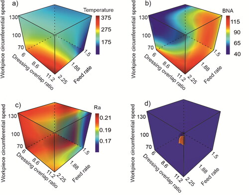
The heat map (Figure 5a–c) shows that slow workpiece circumferential speed n_w combined with high feed rate contributes to high-temperature rise. The behavior of BNA is complex (Figure 5b), but with fast workpiece circumferential speed and a small dressing overlap ratio, low values can be achieved. Small surface roughness occurred with a high dressing overlap ratio and low feed rate (Klocke et al. 2017). Heat maps also show the complicated interaction between the models. For example, having a low temperature and a low BNA will result in high surface roughness. Furthermore, low temperature and surface roughness produce high BNA values. This indicates that the optimal solution is a compromise between the three model outputs.

Surface roughness affects the fatigue life of hardened steels. According to Lai et al. (2016), lower surface roughness increases fatigue life. Therefore, a low value was chosen, Ra 0.185 µm. Figure 5d shows the solution space with the found optimal points. With these constraints, the optimal points are located in the surface area where the feed rate is at the maximum, 2.25 mm/min. The optimal dressing overlap ratio should be high (11.2) and the workpiece circumferential speed should be high (100–130 1/min). Further optimization with respect to grinding costs can be done by finding a point with the minimum cutting power. In this case, this point has a dressing overlap ratio of 11.2 and workpiece circumferential speed of 126.8 1/min with a cutting power of 2280 W.

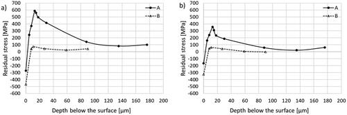
Residual stress depth profiles were carried out from sample A with highest feed rate and dressing values and the lowest workpiece circumferential speed (v_fr 2.25 mm/min, U_d 11.2, n_w 70) and sample B with values closer to the optimal values (v_fr 2.25 mm/min, U_d 11.2, n_w 130). The two residual stress depth profiles for longitudinal (Figure 6a) and tangential direction (Figure 6b) are shown in Figure 6. The surface residual stress values as well as the residual stress depth profiles clearly indicate the effect of the changed n_w when other parameters are kept constant.

Figure 6. Measured longitudinal (a) and tangential (b) residual stress depth profiles from sample A with v_fr 2.25 mm/min, n_w 70, U_d 11.2 and sample B with v_fr 2.25 mm/min, n_w 130, U_d 11.2.

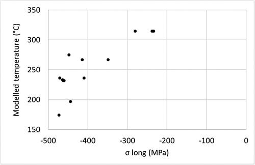
To optimize the process with respect to productivity, the limits of the inequality equations in the optimization problem given in Section “Productivity optimisation” must be defined. This was done using residual stress measurements that were conducted for a chosen subgroup of the experiments. Figure 7 shows the modeled maximum temperature rise in relation to the longitudinal residual stress. From the data, it was determined that residual stress is less than −400 MPa if the temperature rise is less than 250 °C. From Figure 2 this corresponds to BNA values less than 70.

Figure 7. Modeled temperature as a function of longitudinal residual stress.

Discussion

Residual stress measurement showed a good correlation with BNA values for the longitudinal measurement direction, which was also the direction to which the grinding produced higher compressive stresses. In both longitudinal and tangential directions, higher compressive residual stresses were associated with the smaller BNA. Whereas for the tangential residual stresses, the linear relationship with the BNA values was noticed at a certain range of stresses. This might be due to the different sensor sensitivity because different sensors were used in order to measure the different measurement directions. The longitudinal direction showed (Figure 2a) a group of measurements that had high BNA values but low residual stress values. The origins of this outlier group could not be traced. Without it, the relationship between BNA and residual stress would be almost linear in the longitudinal measurement direction.

The chosen parameter combinations in the design of experiment can be considered successful, as it produced grinding burn in the form of decreased residual stresses. In this case, the residual stress values were used as the main threshold value for the grinding burn to occur, since the microstructural changes and their evaluation might be difficult to carry out. In previous study made by the authors (Santa-aho et al., 2023) of the same material as here, with evolving grinding burn, the residual stress state changes much earlier than changes in the microstructure can be seen. The exact type of grinding burns was not studied in detail in this article. Therefore, it is not clear if the changed residual stresses were due to tempering effect or re-hardening. The formation of the final residual stress state during grinding is complicated as there are both thermal and mechanical effects involved, as well as thermal expansion and contraction and material phase transformation if the temperature exceeds the austenitization temperature (Chen et al., 2000).

In addition to residual stresses, the FWHM of the X-ray diffraction peak was measured. It showed similar behavior as residual stresses with respect to BNA. FWHM decreased when BNA increased. FWHM starts to decrease when the temperature reaches the material’s tempering temperature (Zhang et al., 2007). At the same time, hardness starts to decrease also. This raises a question if the limiting grinding temperature could be defined using the tempering temperature indicated by decreasing FWHM value.

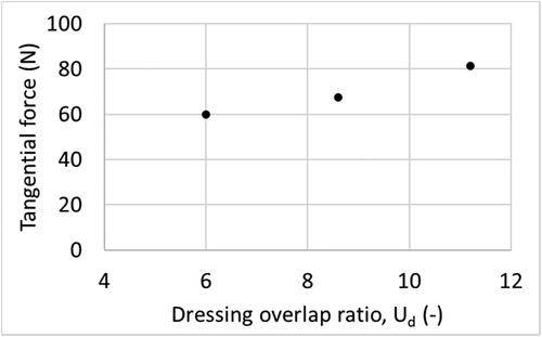
According to Liu et al. (2017), increasing dressing overlap ratio increases tangential grinding force. Similar correlation was observed by calculating the tangential grinding force from measured cutting power.

The tangential force F_t can be calculated from the cutting power P_c by dividing it with the grinding wheel peripheral speed v_s: (10) $$F_t=\frac{P}{v_s}$$(10)

The relationship between tangential force and dressing overlap ratio is shown in Figure 8. This further validates the findings of Liu et al. (2017).

Figure 8. Tangential force as a function of dressing overlap ratio.

ANOVA showed that there are interaction terms present in all three models fitted into the measured data. Both BNA and power models provide accurate estimates shown by a high coefficient of determination. However, the surface roughness model’s coefficient of determination is low (0.738) indicating that the chosen grinding parameters cannot fully explain its behavior. In a similar study by Thanedar et al. (2017) for spark-out time and grinding wheel circumferential speed were included in a model showing better correlation. However, they did not include the dressing overlap ratio which is known to affect the final surface roughness (Liu et al., 2017). Also, the significance of the dressing overlap ratio was highlighted in the main effects plot (Figure 4). This indicates that a more comprehensive model for surface roughness could be produced by including the spark-out time and wheel peripheral velocity into the model proposed in this article.

Heatmaps in Figure 5 show a contradiction between the low values produced by the models. Low temperature and surface roughness could be produced by combining a slow feed rate with a high dressing overlap ratio. However, this would produce high BNA values, which could be unacceptable. Low BNA is produced with low dressing overlap ratio and having the workpiece circumferential speeds above 90 1/min. Yet this would yield high surface roughness. The optimal area is a tradeoff between the model outputs. The result of the optimization can change significantly if more strict restrictions are imposed on the outputs. As the polynomial fits are based on experimental data, their predictive accuracy is good based on the R² values. Next step in the future, is to validate the optimal point which should be done with an experiment conducted with the parameters given by the optimization process.

Conclusions

1. The polynomial fits of BNA and cutting power showed good prediction capability expressed by their R² values. Surface roughness model could be improved by adding spark-out time and wheel peripheral velocity into the model (as done in Thanedar et al., 2017).

2. Dressing overlap-ratio was found to be the most significant grinding parameter with respect to BNA. This signifies the effect of dressing process on the final surface integrity.

3. BNA sensor choice and measurement parameters affect the reliability of the BNA-based quality control. BNA was measured in longitudinal and tangential directions with different sensors and measurement parameters. BNA in the longitudinal measurement direction showed better correlation with the surface residual stresses.

4. Plotted heatmaps showed complicated relationship between the models. The optimal result is a tradeoff between temperature, BNA and surface roughness.

5. An optimization problem was defined with reasonable limiting values based on measurements that produced a set of optimal points. The optimal point that minimizes the cutting power was chosen as the final optimal point which provides the optimal grinding parameters; the feed rate is at the maximum, 2.25 mm/min, the dressing overlap ratio should be high (11.2) and the workpiece peripheral velocity should be high (100–130 1/min).

Nomenclature
α	=	workpiece thermal diffusivity
ε	=	heat partition ratio
µ	=	cutting force ratio
ρ	=	workpiece density
θm	=	maximum temperature rise
ae	=	depth of cut
bw	=	grinding wheel width
cp	=	workpiece specific heat capacity
de	=	equivalent wheel diameter
ds	=	grinding wheel diameter
dw	=	workpiece diameter
E*	=	combined elastic modulus
E1	=	Work modulus
E2	=	Wheel modulus
ν1	=	Work Poisson’s ratio
ν2	=	Wheel Poisson’s ratio
Ft	=	tangential force
k	=	workpiece thermal conductivity
lc	=	real contact length
nw	=	workpiece circumferential speed
Pc	=	cutting power
Qw	=	material removal rate
Q’w	=	specific material removal rate
qw	=	heat flux into the workpiece
r	=	workpiece radius
Ra	=	average mean surface roughness
Rr	=	roughness factor
Ud	=	dressing overlap ratio
vfr	=	radial feed rate
vs	=	grinding wheel peripheral speed
vw	=	workpiece peripheral velocity
ANOVA	=	Analysis of variance
BN	=	Barkhausen noise
BNA	=	maximum values for BN average RMS
DOE	=	design of experiments
FWHM	=	full width half maximum of XRD profiles
NDT	=	Nondestructive testing
RMS	=	root mean square of voltage signal
SQLSP	=	sequential least squared programming
XRD	=	X-ray diffraction

Disclosure statement

No potential conflict of interest was reported by the author(s).

Additional information

Funding

The support of participants of the ÄVE-project funded by Business Finland is appreciated. Additionally, this work was supported by a grant provided by K.F. and Maria Dunderberg Foundation.

References

- Antony, J. (2014) Design of Experiments for Engineers and Scientists. Elsevier.
- Azarhoushang, B.; Daneshi, A.; Lee, D.H. (2017) Evaluation of thermal damages and residual stresses in dry grinding by structured wheels. Journal of Cleaner Production, 142: 1922–1930. doi:10.1016/j.jclepro.2016.11.091
- Canale, L.C.F.; Vatavuk, J.; Totten, G.E.; Luo, X. (2014) Problems associated with heat treating, In ASM Handbook, Steel Heat Treating Technologies, Vol. 4B. doi:10.31399/asm.hb.v04b.a0005967
- Chen, X.; Rowe, W.B.; McCormack, D.F. (2000) Analysis of the transitional temperature for tensile residual stress in grinding. Journal of Materials Processing Technology, 107(1-3): 216–221. doi:10.1016/S0924-0136(00)00692-0
- Citti, P.; Molinari, P.; Giorgetti, A.; Polidoro, A.; Pompei, L.; Arcidiacono, G. (2021) Design and validation of low-cost handling equipment for the use of barkhausen noise testing in worm gears grinding burn detection. IOP Conference Series: Materials Science and Engineering 1038(1): 012066. 10.1088/1757-899X/1038/1/012066
- Hamdi, H.; Zahouani, H.; Bergheau, J.M. (2004) Residual stresses computation in a grinding process. Journal of Materials Processing Technology, 147(3): 277–285. 10.1016/S0924-0136(03)00578-8
- Hashimoto, F.; Guo, Y.B.; Warren, A.W. (2006) Surface integrity difference between hard turned and ground surfaces and its impact on fatigue life. CIRP Annals, 55(1): 81–84. 10.1016/S0007-8506(07)60371-0
- Hauk, V. (1997) Structural and Residual Stress Analysis by Nondestructive Methods. Elsevier,
- Heinzel, J.; Sackmann, D.; Karpuschewski, B. (2019) Micromagnetic analysis of thermally induced influences on surface integrity using the burning limit approach. Journal of Manufacturing and Materials Processing, 3(4): 93. doi:10.3390/jmmp3040093
- Jedamski, R.; Heinzel, J.; Rößler, M.; Epp, J.; Eckebrecht, J.; Gentzen, J.; Putz, M.; Karpuschewski, B. (2020) Potential of magnetic barkhausen noise analysis for in-process monitoring of surface layer properties of steel components in grinding. TM - Technisches Messen, 87(12): 787–798. doi:10.1515/teme-2020-0048
- Karpuschewski, B.; Inasaki, I. (2006) Monitoring systems for grinding processes. In Condition Monitoring and Control for Intelligent Manufacturing. Springer Series in Advanced Manufacturing, Wang L. and Gao R.X. (Eds.), London: Springer. doi:10.1007/1-84628-269-1_4
- Karpuschewski, B.; Bleicher, O.; Beutner, M. (2011) Surface integrity inspection on gears using barkhausen noise analysis, 1st CIRP Conference on Surface Integrity (CSI). Procedia Engineering, 19: 162–171. doi:10.1016/j.proeng.2011.11.096
- Karpuschewski, B.; Beutner, M.; Eckebrecht, J.; Heinzel, J.; Hüsemann, T. (2020) Surface integrity aspects in gear manufacturing, 5th CIRP CSI 2020. Procedia CIRP, 87: 3–12. doi:10.1016/j.procir.2020.05.112
- Kleber, X.; Vincent, A. (2004) On the role of residual internal stresses and dislocations on barkhausen noise in plastically deformed steel. NDT & E International, 37(6): 439–445. 10.1016/j.ndteint.2003.11.008
- Kopac, J.; Krajnik, P. (2006) High-performance grinding—a review. Journal of Materials Processing Technology, 175(1-3): 278–284. 10.1016/j.jmatprotec.2005.04.010
- Koster, W.P.; Field, M.; Kahles, J.F.; Fritz, L.J.; Gatto, L.R. (1969) Surface integrity of machined structural components. Final Technical rep1 Feb 1968-30 Nov 1969.
- Liu, Y.; Gong, S.; Li, J.; Cao, J. (2017) Effects of dressed wheel topography on patterned surface textures and grinding forces. The International Journal of Advanced Manufacturing Technology, 93(5-8): 1751–1760. doi:10.1007/s00170-017-0647-9
- Malkin, S.; Guo, C. (2007) Thermal analysis of grinding. CIRP Annals, 56(2): 760–782. doi:10.1016/j.cirp.2007.10.005
- Malkin, S.; Guo, C. (2008) Grinding Technology: Theory and Application of Machining with Abrasives. Industrial Press Inc.
- Marinescu, I.D.; Rowe, W.B.; Dimitrov, B.; Ohmori, H. (2013) Tribology of Abrasive Machining Processes. William Andrew.
- Micietova, A.; Neslusan, M.; Cep, R.; Ochodek, V.; Micieta, B.; Pagac, M. (2017) Detection of grinding burn through the high and low frequency barkhausen noise. Tehnički Vjesnik, 24(Suppl. 1): 71–77. doi:10.17559/TV-20140203083223
- Moorthy, V.; Shaw, B.A.; Evans, J.T. (2003) Evaluation of tempered induced changes in the hardness profile of case-carburised en36 steel using magnetic barkhausen noise analysis. NDT & E International, 36(1): 43–49. doi:10.1016/S0963-8695(02)00070-1
- Nakah, B. (2017) Material characterization using barkhausen noise analysis technique—a review. Indian Journal of Science and Technology, 10(14): 1–10. doi:10.17485/ijst/2017/v10i14/109697
- Neslušan, M.; Čížek, J.; Kolařík, K.; Minárik, P.; Čilliková, M.; Melikhova, O. (2017) Monitoring of grinding burn via barkhausen noise emission in case-hardened steel in large-bearing production. Journal of Materials Processing Technology, 240: 104–117. 10.1016/j.jmatprotec.2016.09.015
- Parrish, G. (1999) Carburizing: Microstructures and Properties. ASM International.
- Sackmann, D.; Heinzel, J.; Karpuschewski, B. (2020) An approach for a reliable detection of grinding burn using the barkhausen noise multi-parameter analysis. Procedia CIRP, 87: 415–419. 10.1016/j.procir.2020.02.076
- Santa-aho, S.; Sorsa, A.; Ruusunen, M.; Vippola, M, Tampere University of Technology (2023) Grinding burn classification with surface barkhausen noise measurements. Papers of the ECNDT 2023. Research and Review Journal of Nondestructive Testing, 1(1). 10.58286/28170
- Schajer, G. (2013) Practical Residual Stress Measurement Methods. Hoboken: Wiley.
- SFS-EN 15305 (2008) Non-destructive testing: test method for residual stress analysis by X-ray diffraction. SUOMEN STANDARDISOIMISLIITTO SFS
- Shaw, B.A.; Aylott, C.; O’Hara, P.; Brimble, K. (2003) The role of residual stress on the fatigue strength of high performance gearing. International Journal of Fatigue, 25(9-11): 1279–1283. 10.1016/j.ijfatigue.2003.08.014
- Stewart, D.M.; Stevens, K.J.; Kaiser, A.B. (2004) Magnetic barkhausen noise analysis of stress in steel. Current Applied Physics, 4(2-4): 308–311. 10.1016/j.cap.2003.11.035
- Teixeira, P.H.; Rego, R.R.; Pinto, F.W.; de Oliveira Gomes, J.; Löpenhaus, C. 2019, Application of hall effect for assessing grinding thermal damage. Journal of Materials Processing Technology, 270: 356–364. doi:10.1016/j.jmatprotec.2019.02.019
- Thanedar, A.; Dongre, G.G.; Joshi, S.S. (2019) Analytical modelling of temperature in cylindrical grinding to predict grinding burns. International Journal of Precision Engineering and Manufacturing, 20(1): 13–25. doi:10.1007/s12541-019-00037-9
- Thanedar, A.; Dongre, G.G.; Singh, R.; Joshi, S.S. (2017) Surface integrity investigation including grinding Burns Using Barkhausen Noise (BNA). Journal of Manufacturing Processes, 30: 226–240. 10.1016/j.jmapro.2017.09.026
- Tomkowski, R.; Sorsa, A.; Santa-aho, S.; Lundin, P.; Vippola, M. (2019) Statistical evaluation of Barkhausen Noise Testing (BNT) for ground samples. Sensors, 19(21): 4716. doi:10.3390/s19214716
- Torrance, A.A. (1979) Metallurgical effects associated with grinding. In Proceedings of the Nineteenth International Machine Tool Design and Research Conference, 637–644. Palgrave, London.
- Turner, J.R.; Thayer, J. (2001) Introduction to Analysis of Variance: Design, Analysis & Interpretation: Design, Analysis & Interpretation. Sage.
- Zhang, Z.P.; Qi, Y.H.; Delagnes, D.; Bernhart, G. (2007) Microstructure variation and hardness diminution during low cycle fatigue of 55NiCrMoV7 steel. Journal of Iron and Steel Research International, 14(6): 68–73. 10.1016/S1006-706X(07)60093-4
- As, S.; Skallerud, B.; Tveiten, B. (2008) Surface roughness characterization for fatigue life predictions using finite element analysis. International Journal of Fatigue, 30(12): 2200–2209. 10.1016/j.ijfatigue.2008.05.020