Collaborative Insurance with Stop-Loss Protection and Team Partitioning

Abstract

Denuit (2019, 2020a) demonstrated that conditional mean risk sharing introduced by Denuit and Dhaene (2012) is the appropriate theoretical tool to share losses in collaborative peer-to-peer insurance schemes. Denuit and Robert (2020a, 2020b, 2021) studied this risk sharing mechanism and established several attractive properties including linear approximations when total losses or the number of participants get large. It is also shown there that the conditional expectation defining the conditional mean risk sharing is asymptotically increasing in the total loss (under mild technical assumptions). This ensures that the risk exchange is Pareto-optimal and that all participants have an interest to keep total losses as small as possible. In this article, we design a flexible system where entry prices can be made attractive compared to the premium of a regular, commercial insurance contract and participants are awarded cash-backs in case of favorable experience while being protected by a stop-loss treaty in the opposite case. Members can also be grouped according to some meaningful criteria, resulting in a hierarchical decomposition of the community. The particular case where realized losses are allocated in proportion to the pure premiums is studied.

1. INTRODUCTION AND MOTIVATION

In collaborative, peer-to-peer (P2P) insurance, participants agree to pool the risks they face. P2P insurance thus builds on the fundamental principle of mutuality at the origin of insurance without the equity buffer provided by insurer’s capital. When large losses occur, pooling can be restricted to the first layer so that the scheme can avoid running out of money. Higher losses are then transferred to a third party, typically an insurance or reinsurance company. In this article, we consider that the pool retains the total losses up to a given threshold and the part above the threshold is covered by some (re-)insurer with the help of a stop-loss protection. Unclaimed money can be paid back, given to a charity, or used to fund a common project to which the community adheres. We refer to Clemente and Marano (2020) and the references therein for an overview of P2P insurance.

Collaborative, P2P insurance schemes may well become an additional sales channel, complementing classical ones such as brokers, direct, bank, as well as blank products provided to a retailer in business-to-business transactions, between companies rather than between a company and individual consumer. This new channel also addresses one of the key challenges faced by the insurance industry in the 21st century: offering appropriate coverage to every customer that meets his or her own personal expectations. In that respect, the parallel with the blend of consumers’ profiles existing in electricity markets seems to be instructive. These profiles range from consumers staying with the ex-monopolistic provider, buying electricity produced from coal or nuclear plants, corresponding to policyholders buying traditional contracts, sold by brokers or through large bank networks (or by direct insurers if price is an important aspect). At the other extremity, we find those consumers buying shares in windmill projects near to their residence, corresponding to individuals joining a mutual insurer owned by its members. In between, we pass through (i) consumers buying green electricity, corresponding to policyholders opting for a product supporting sustainable development; for example, through ethical investments, still sold by classical insurance actors; (ii) prosumers installing solar panels on their roof and equipping their buildings with batteries, staying connected to the public electricity network to face the extreme case where their own system does not suffice, corresponding to individuals prone to self-insurance, wishing to access high deductibles that reduce premiums to a large extent; and (iii) local energy communities providing inhabitants with electricity produced nearby by their members, corresponding to P2P insurance communities. There is strong potential for developing insurance offerings along these lines from an economic point of view, because the yearly electricity bill for a typical household is of the same order as car insurance premiums. Further, younger generations question existing models, including those dominating the insurance industry, and it is of crucial importance to address their concerns.

Setting a collaborative insurance scheme raises the following question: how to fairly share, in an understandable and transparent way, that part of the premium that has not been used to cover the claims. Insurance risks are heterogeneous, and equally sharing the total losses among participants may well appear to be unfair. To be successful, P2P insurance schemes require an appropriate risk sharing mechanism recognizing the different distributions of the risks brought to the pool. Intuitively speaking, participants pooling “smaller” or “less variable” risks should contribute less to the realized total loss. Denuit (2019) proposed a simple and mathematically correct solution based on the conditional mean risk sharing rule introduced by Denuit and Dhaene (2012). Based on the concept of mean value, this sharing rule is quite intuitive because most participants have at least a vague idea about averaging and its risk-reducing effect. Because participants can be informed when they enter the pool about the amount they will have to contribute as a function of the total realized loss, this approach ensures full transparency.

Let us explain how such a system operates. Consider n participants in an insurance pool, numbered $i=1,2,\dots ,n.$ Each of them faces a risk X_i. By risk we mean a non-negative random variable representing a monetary loss caused by some insurable peril over one period (a calendar year, say). Henceforth, we use the notation $S={\sum }_{i=1}^n{X}_i$ for the total risk of the pool. In the conditional mean risk sharing (or allocation) proposed by Denuit and Dhaene (2012), each participant contributes ex post the amount $\mathrm{E}[X_i|S=s]$ where $s={\sum }_{i=1}^n{x}_i$ is the sum of the realizations $x_1,x_2,\dots ,x_n$ of $X_1,X_2,\dots ,X_n.$ Clearly, the conditional mean risk sharing allocates the full risk S because we obviously have ${\sum }_{i=1}^n\mathrm{E}[X_i|S]=S.$ That is, participant i must contribute the expected value of the risk X_i he or she brings to the pool, given the total loss S experienced by the entire community. Stated differently, the contribution of each participant is the average part of the total loss S that can be attributed to the risk he or she brought to the pool.

The key point to explain to the members of a P2P insurance community is that the actual realization of X_i is mostly due to chance and only partly reveals the underlying magnitude of the risk brought to the community. Over one period, the conditional mean risk sharing splits the risk X_i into a random part $X_i-\mathrm{E}[X_i|S]$ shared among participants by virtue of the mutuality (or random solidarity) principle and a structural part $\mathrm{E}[X_i|S]$ to be supported by participant i, individually. Formally, the risk X_i brought by participant i is decomposed into (1.1) $$X_i=\underset{=\text{structural}\mathrm{ }\text{part}}{\underbrace{\mathrm{E}\left[X_i\right|S]}}+\underset{=\text{random}\mathrm{ }\text{departure}\mathrm{ }{\mathcal{E}}_i}{\underbrace{X_i-\mathrm{E}\left[X_i\right|S]}}.$$(1.1)

Both terms entering this split are uncorrelated and random departures ${\mathcal{E}}_i$ always sum to 0. The latter property ensures that the community bears its own risk, without transferring (part of) it to another economic agent.

In commercial insurance, the variations in S are absorbed by insurer’s capital and individual i must contribute a fixed amount to compensate the cost of insured events, equal to the pure premium $\mathrm{E}[X_i]$ supplemented with shareholder’s profit for providing the risk-bearing capital. With P2P insurance, each participant must contribute ex post the amount $\mathrm{E}[X_i|S]$ to the pool, whereas the random departures ${\mathcal{E}}_1,{\mathcal{E}}_2,\dots ,{\mathcal{E}}_n$ entering the decomposition (1.1(1.1) $$X_i=\underset{=\text{structural}\mathrm{ }\text{part}}{\underbrace{\mathrm{E}\left[X_i\right|S]}}+\underset{=\text{random}\mathrm{ }\text{departure}\mathrm{ }{\mathcal{E}}_i}{\underbrace{X_i-\mathrm{E}\left[X_i\right|S]}}.$$(1.1) ) are reallocated among them according to the mutuality principle. The expected contribution is equal to the expected loss; that is, $$\mathrm{E}\left[\mathrm{E}\right[X_i\left|S\right]]=\mathrm{E}[X_i],i=1,2,\dots ,n.$$

The conditional mean risk allocation is thus considered to be fair: On average, individual contributions match the corresponding losses so that no participant gains in the operation. Stated otherwise, there are no transfers among participants to the pool, on average, so that each of them bears the consequence of their own risk.

However, several issues need to be addressed before a possible implementation of the conditional mean risk sharing in collaborative insurance. First and foremost, the entry price must be attractive and an upper limit should be placed on personal contributions to convince participants to join the community. This is especially important when the new scheme is launched. Unfortunately, this is not guaranteed with the system designed by Denuit (2020a) where individual contributions derive from the total amount of retention selected by the community. The present article is innovative in that we start from the amounts paid ex ante by participants (replacing premiums charged by commercial insurers) and design the system in such a way that no additional contribution is needed ex post (thanks to the stop-loss treaty protecting the community) and a cash-back can be awarded at the end of the period, in case of favorable experience. If the organizer can design the system in such a way that the probability of awarding such a cash-back is high enough, it is very likely that the cost of the coverage will be smaller than the entry price paid ex ante.

In addition, participants are often grouped to “teams” based on existing networks (family or relatives, for instance), common economic interests or geographic location. We adapt the system to account for these two levels: the intermediate group level in addition to the individual level. We also discuss possible simplifications to the conditional mean risk sharing rule. Precisely, we show that this sharing may reduce to a simple proportional allocation of losses, according to pure premiums. Notice that participants can also opt for this allocation rule for simplicity. In the two-level case, the theoretically correct conditional mean risk sharing rule can be applied at the upper level (to ensure fairness between groups, avoiding any undue transfer), whereas within the groups the simpler proportional mean risk allocation may be applied (even if it is not formally supported by theoretical arguments).

The remainder of this article is organized as follows. Section 2 is devoted to the design of the proposed collaborative P2P insurance scheme. In Section 3, we adapt this scheme to the case where participants are partitioned into subgroups because this is often the case in practice. Section 4 proposes numerical illustrations. Section 5 briefly discusses the result obtained in this article.

2. DESIGN OF THE P2P INSURANCE SCHEME

2.1. Assumptions

Throughout this article, we assume that

1. the losses X_i are valued in $[0,\infty )$ and obey zero-augmented absolutely continuous distributions; that is, $\mathrm{P}[X_i=0]>0$ and X_i possesses a probability density function $f_{X_i|X_i>0}$ over $(0,\infty ).$

2. the losses $X_1,\dots ,X_n$ are mutually independent, with finite means $\mathrm{E}[X_i]={\mu }_i>0.$

3. the conditional expectations $\mathrm{E}[X_i|S]$ are continuously increasing in S for all i so that the functions $s\mapsto \mathrm{E}[X_i|S=s]$ are one-to-one.

Let us comment on these hypotheses. Assumption (i) is very general. It corresponds to the representation of insurance risks within the individual model of risk theory. Assumption (ii) requires a careful examination given the nature of collaborative insurance. Because P2P insurance communities typically gather individuals sharing some familial, social, or entrepreneurial relationship, we can expect that members of the same group have similar risk profiles, to some extent, because they live in the same area or belong to the same socio-economic class, for instance. Including these characteristics in the risk classification plan—that is, letting the distribution of X_i depend on these risk factors through an appropriate regression model—we can end up with independent losses $X_1,\dots ,X_n$ given the risk factors. This is the case for car or home insurance, for instance. However, independence is sometimes unrealistic so that the approach developed in this article does not apply. This is, for instance, the case for the cover against natural catastrophes where geographic proximity rules out independence. Considering health insurance, losses corresponding to members of the same family may be correlated by hidden risk factors so that assumption (ii) becomes questionable.

Assumption (iii) ensures that the conditional expectations $\mathrm{E}[X_i|S]$ are comonotonic random variables; that is, they all move in the same direction with the total loss S, increasing when S gets larger and decreasing when S gets smaller. Properties of such random variables have been thoroughly reviewed by Dhaene et al. (2002a,b). Denuit (2020a) demonstrated that comonotonicity allows us to derive the allocation of S to the n participants. See also Denuit (2020b) for related results. From a theoretical point of view, requiring that each $\mathrm{E}[X_i|S]$ is a nondecreasing function of S ensures that the conditional mean risk sharing is Pareto-optimal for expected utility maximizers, as shown by Denuit and Dhaene (2012). In practice, this means that all participants have an interest in keeping S as low as possible because their contributions increase with total losses.

It is important to stress that assumption (iii) is not always valid. Counterexamples are easy to build with discrete losses X_i assuming just a few values or with different supports (because the value of s may bring some information about the realization of individual losses in this simplistic setting). General conditions on the distributions of the random variables X_i ensuring that $\mathrm{E}[X_i|S]$ is nondecreasing in S are difficult to establish. A sufficient condition is that the independent random variables X_i possess log-concave densities, as established by Efron (1965). Under mild technical conditions, Denuit and Robert (2020a) showed that assumption (iii) is fulfilled at the limit when the number n of participants is large enough.

Notice that X_i corresponds to the risk brought by participant i to the pool, after deduction of some individual retention. For instance, this participant could specify perclaim or aggregate deductibles so that X_i only corresponds to the excess over the individual retention level. In addition, the pool could (re-)insure part of X_i in case large losses may occur, with the help of any individual treaty (such as excess of loss, for instance). In this case, the price of the treaty must simply be added to the entry price discussed in the next sections.

2.2. Entry Price, Stop-Loss Protection and Cash-Back Mechanism

To ensure that the system does not run out of money, participants must pay a provision, ex ante so that the sum of the provisions is enough to cover the entirety of the losses, in all cases. This means that the upper layer of the total losses is ceded to a (re-)insurer and that collaborative insurance is restricted to the lower layer.

Henceforth, π_i denotes the provision paid ex ante by participant i bringing loss X_i to the pool. This is the entry price to join the community. The amount π_i is obtained by applying a premium calculation principle and only depends on the distribution of X_i. Expected value and variance principles will be used in the next sections, but other premium calculation principles can be envisaged in some specific applications.

The total amount ${\sum }_{i=1}^n{\pi }_i$ of provisions must be enough to cover the aggregate loss S of the pool, in all cases. This is made possible by buying a stop-loss protection of the upper layer from a (re-)insurance company. Precisely, denoting the retention capacity of the P2P insurance community as w, the upper layer $(w,\infty )$ is ceded to a (re-)insurer in exchange for a premium ${\pi }_{\text{SL}}.$ The lower layer $(0,w)$ is kept within the community. Ex post—that is, at the end of the coverage period—a cash-back mechanism operates to restore fairness (see Subsection 2.6.4 for a formal discussion of the notion of fairness in P2P insurance schemes). In case of a favorable experience that—is, if S < w the surplus w–S is distributed among participants, as explained next. Alternatively, unclaimed money can also be given to a charity or used to fund a common project to which the community adheres.

2.3. Determination of the Retention Capacity of the P2P Community

The amount w retained by the pool is the solution to the equation (2.1) $$\sum _{i=1}^n{\pi }_i-(1+{\theta }_{\text{SL}})\mathrm{E}\left[{(S-w)}_{+}\right]=w.$$(2.1)

That is, (2.1(2.1) $$\sum _{i=1}^n{\pi }_i-(1+{\theta }_{\text{SL}})\mathrm{E}\left[{(S-w)}_{+}\right]=w.$$(2.1) ) ensures that the total income ${\sum }_{i=1}^n{\pi }_i$ allows the organizer to pay for losses up to w and to transfer the upper layer $(w,\infty )$ to a (re-)insurer in exchange for the premium (2.2) $${\pi }_{\text{SL}}={\pi }_{\text{SL}}(w)=(1+{\theta }_{\text{SL}})\mathrm{E}\left[{(S-w)}_{+}\right],$$(2.2) where w fulfills Equation (2.1)(2.1) $$\sum _{i=1}^n{\pi }_i-(1+{\theta }_{\text{SL}})\mathrm{E}\left[{(S-w)}_{+}\right]=w.$$(2.1) . The cash-back mechanism then restores fairness ex post, when S < w.

The next result establishes the existence and uniqueness of the solution w to Equation (2.1)(2.1) $$\sum _{i=1}^n{\pi }_i-(1+{\theta }_{\text{SL}})\mathrm{E}\left[{(S-w)}_{+}\right]=w.$$(2.1) , provided π_i is not too small.

Property 2.1.

If the inequality ${\pi }_i>(1+{\theta }_{\text{SL}})\mathrm{E}[X_i]$ is valid for all i, then the solution w to Equation (2.1)(2.1) $$\sum _{i=1}^n{\pi }_i-(1+{\theta }_{\text{SL}})\mathrm{E}\left[{(S-w)}_{+}\right]=w.$$(2.1) exists and is unique. Moreover, it fulfills $F_S(w)>\frac{{\theta }_{\text{SL}}}{1+{\theta }_{\text{SL}}}.$

Proof.

Consider the continuous function $\phi$ defined as $$\phi (\xi )=\xi +(1+{\theta }_{\text{SL}})\mathrm{E}\left[{(S-\xi )}_{+}\right].$$

Equation (2.1)(2.1) $$\sum _{i=1}^n{\pi }_i-(1+{\theta }_{\text{SL}})\mathrm{E}\left[{(S-w)}_{+}\right]=w.$$(2.1) then requires one to find where $\phi$ crosses the horizontal line at height ${\sum }_{i=1}^n{\pi }_i.$ Notice that $$\sum _{i=1}^n{\pi }_i>\sum _{i=1}^n(1+{\theta }_{\text{SL}})\mathrm{E}\left[X_i\right]=\phi (0)$$ so that the solution cannot be located at the origin. Because $$\phi \prime (\xi )=1-(1+{\theta }_{\text{SL}}){\overline{F}}_S(\xi ),$$ the function $\phi$ is increasing if $$\phi \prime (\xi )>0\iff {\overline{F}}_S(\xi )<\frac{1}{1+{\theta }_{\text{SL}}}\iff \xi >F_S^{-1}\left(\frac{{\theta }_{\text{SL}}}{1+{\theta }_{\text{SL}}}\right)={\xi }_0.$$

Thus, the function $\phi$ starts below ${\sum }_{i=1}^n{\pi }_i$ at the origin and then decreases until ξ₀ where it reaches its minimum before starting to increase at ξ₀. Because $\phi (\xi )\to \infty$ as $\xi \to \infty ,$ there must be a unique solution to Equation (2.1)(2.1) $$\sum _{i=1}^n{\pi }_i-(1+{\theta }_{\text{SL}})\mathrm{E}\left[{(S-w)}_{+}\right]=w.$$(2.1) , as announced. □

If we consider that the reinsurance company is the analogue of a wholesale dealer on the insurance market, the inequality ${\pi }_i>(1+{\theta }_{\text{SL}})\mathrm{E}[X_i]$ assumed in Property 2.1 means that the retail price π_i cannot fall below the wholesale, or factory, price $(1+{\theta }_{\text{SL}})\mathrm{E}[X_i].$ This constraint thus appears to be reasonable in our context.

Notice that $F_S(w)$ is the probability that there is some relief to be distributed among participants. We thus see from Property 2.1 that the probability that the cash-back mechanism operates is at least equal to $\frac{{\theta }_{\text{SL}}}{1+{\theta }_{\text{SL}}}.$

2.4. Individual Contributions to the Stop-Loss Cover

Proceeding as in Denuit (2020a), each participant is liable for an amount (2.3) $$w_i=F_{\mathrm{E}\left[X_i\right|S]}^{-1}(F_S(w))\mathrm{ }\text{with}\mathrm{ }\sum _{i=1}^n{w}_i=w.$$(2.3)

The amounts $w_1,\dots ,w_n$ defined in this way are such that (2.4) $${(S-w)}_{+}=\sum _{i=1}^n(\mathrm{E}[X_i\left|S\right]-w_i{)}_{+}\mathrm{ }\text{and}\mathrm{ }{(w-S)}_{+}=\sum _{i=1}^n(w_i-\mathrm{E}[X_i\left|S\right]{)}_{+}.$$(2.4)

The key to understanding decompositions appearing in (2.4(2.4) $${(S-w)}_{+}=\sum _{i=1}^n(\mathrm{E}[X_i\left|S\right]-w_i{)}_{+}\mathrm{ }\text{and}\mathrm{ }{(w-S)}_{+}=\sum _{i=1}^n(w_i-\mathrm{E}[X_i\left|S\right]{)}_{+}.$$(2.4) ) is as follows: The total loss S is not larger than w with probability $F_S(w).$ Because each $\mathrm{E}[X_i|S]$ is a continuously increasing function of S, we have $$S\le w\iff \mathrm{E}\left[X_i\right|S]\le w_i\mathrm{ }\text{for}\mathrm{ }i=1,2,\dots ,n,$$ where w_i is defined according to (2.3(2.3) $$w_i=F_{\mathrm{E}\left[X_i\right|S]}^{-1}(F_S(w))\mathrm{ }\text{with}\mathrm{ }\sum _{i=1}^n{w}_i=w.$$(2.3) ). This shows that the identities (2.4(2.4) $${(S-w)}_{+}=\sum _{i=1}^n(\mathrm{E}[X_i\left|S\right]-w_i{)}_{+}\mathrm{ }\text{and}\mathrm{ }{(w-S)}_{+}=\sum _{i=1}^n(w_i-\mathrm{E}[X_i\left|S\right]{)}_{+}.$$(2.4) ) are indeed valid. The total surplus ${(w-S)}_{+}$ can thus be distributed among participants according to (2.4(2.4) $${(S-w)}_{+}=\sum _{i=1}^n(\mathrm{E}[X_i\left|S\right]-w_i{)}_{+}\mathrm{ }\text{and}\mathrm{ }{(w-S)}_{+}=\sum _{i=1}^n(w_i-\mathrm{E}[X_i\left|S\right]{)}_{+}.$$(2.4) ). Precisely, participant i is granted an amount $${\text{cash}-\text{back}}_i=(w_i-\mathrm{E}[X_i\left|S\right])\mathrm{I}[S\le w]={(w_i-\mathrm{E}[X_i\left|S\right])}_{+}$$ that can be used to reduce the cost of next-year coverage, or given to the charity of his or her choice.

Considering (2.4(2.4) $${(S-w)}_{+}=\sum _{i=1}^n(\mathrm{E}[X_i\left|S\right]-w_i{)}_{+}\mathrm{ }\text{and}\mathrm{ }{(w-S)}_{+}=\sum _{i=1}^n(w_i-\mathrm{E}[X_i\left|S\right]{)}_{+}.$$(2.4) ), The initial contribution π_i in (2.6(2.6) $${\pi }_i=(1+{\theta }_{\mathrm{P}2\mathrm{P}})\mathrm{E}\left[X_i\right],$$(2.6) ) can then be split into $${\pi }_i={\pi }_i^{\mathrm{P}2\mathrm{P}}+{\pi }_i^{\text{SL}}\mathrm{ }\text{where}\mathrm{ }{\pi }_i^{\text{SL}}=(1+{\theta }_{\text{SL}})\mathrm{E}\left[{(\mathrm{E}[X_i\left|S\right]-w_i)}_{+}\right].$$

The total loss S is well covered: the upper layer $(w,\infty )$ is transferred to the (re-)insurer for the payment ${\pi }_i^{\text{SL}}$ and $$\sum _{i=1}^n{\pi }_i-\sum _{i=1}^n{\pi }_i^{\text{SL}}=w\mathrm{ }\text{with}\mathrm{ }{\pi }_{\text{SL}}=\sum _{i=1}^n{\pi }_i^{\text{SL}},$$ by virtue of (2.1(2.1) $$\sum _{i=1}^n{\pi }_i-(1+{\theta }_{\text{SL}})\mathrm{E}\left[{(S-w)}_{+}\right]=w.$$(2.1) ). Thus, the lower layer $(0,w)$ is covered by the contributions ${\pi }_i^{\mathrm{P}2\mathrm{P}}$ paid ex ante by participants Because (2.1(2.1) $$\sum _{i=1}^n{\pi }_i-(1+{\theta }_{\text{SL}})\mathrm{E}\left[{(S-w)}_{+}\right]=w.$$(2.1) ) ensures that the identity ${\sum }_{i=1}^n{\pi }_i^{\mathrm{P}2\mathrm{P}}={\sum }_{i=1}^n{w}_i=w$ holds true. However, ${\pi }_i^{\mathrm{P}2\mathrm{P}}$ is not necessarily equal to w_i for every participant. In the next sections, how this mismatch can be solved will be shown. First, we compare the proposed mechanism to insurance.

2.5. Comparison with Insurance

Let us carefully compare traditional insurance with its collaborative counterpart. In both cases, the loss X_i caused by the peril under consideration is reimbursed to individual i so that we concentrate on premiums or provisions paid ex ante and possible cash-backs awarded ex post, accompanying collaborative insurance.

2.5.1. Classical Insurance Solution

In a traditional insurance scheme involving one insurance company covering n policyholders for a given peril, individual premiums ${\pi }_i^{\text{comm}}$ are loaded; that is, ${\pi }_i^{\text{comm}}>\mathrm{E}[X_i].$ The sum of individual premiums ${\sum }_{i=1}^n{\pi }_i^{\text{comm}}$ is used to pay for claims filed by the policyholders amounting to S. A solvency capital is used to face situations where S exceeds the total premium collected and ${\pi }_i^{\text{comm}}$ comprises the dividends to be paid to stockholders with risk-bearing capacities. As an alternative to maintaining a sufficiently high capital buffer, the insurance company can also buy reinsurance or implement other risk mitigation mechanisms. The corresponding cost is then included in ${\pi }_i^{\text{comm}}.$

2.5.2. Collaborative Insurance and Cash-Back Mechanism

In the P2P insurance scheme proposed in this article, involving one community of n participants and a (re-)insurance company protecting the upper risk layer, individual provisions π_i are paid ex ante. The key advantage of the system proposed in this article is that π_i does not depend on the number of participants or on the losses X_k, $k\ne i,$ they bring to the community but depends only on the distribution of the loss for participant i. Exactly as in traditional insurance, the inclusion of a new participant leaves π_i unchanged. But recruiting new members modifies the distribution of S that materializes in the value of the retention level w solving Equation (2.1)(2.1) $$\sum _{i=1}^n{\pi }_i-(1+{\theta }_{\text{SL}})\mathrm{E}\left[{(S-w)}_{+}\right]=w.$$(2.1) and impacts on the cash-back mechanism.

Notice also that the individual retention level w_i defined according to (2.3(2.3) $$w_i=F_{\mathrm{E}\left[X_i\right|S]}^{-1}(F_S(w))\mathrm{ }\text{with}\mathrm{ }\sum _{i=1}^n{w}_i=w.$$(2.3) ) can be rewritten as $$w_i=\mathrm{E}\left[X_i\right|S=F_S^{-1}(F_S(w))]=\mathrm{E}[X_i|S=w],$$ which obviously sums to w. This is because $s\mapsto \mathrm{E}[X_i|S=s]$ is continuously increasing in s; we refer the interested reader to Denuit (2020a) for more general formulas. This shows how recruiting new members impacts individual i: The provision π_i paid ex ante is left unchanged but the cash back mechanism generating the end-of-period cashflow is modified. The latter may be more or less favorable to the participant, depending on the community he or she joins. If the organizer of the collaborative insurance scheme is able to charge ${\pi }_i\le {\pi }_i^{\text{comm}}$ ex ante then participants can only win by joining the community.

2.5.3. Risk Classification

As discussed earlier, risk classification is still needed in collaborative insurance. This means that the organizer must have an accurate loss model at its disposal, given an appropriate probability distribution for every loss brought to the community. In that respect, collaborative insurance is similar to traditional insurance: A sufficiently accurate risk classification plan and appropriate underwriting rules are needed to prevent adverse selection. Let us mention that even if adverse selection effects do not threaten the organizer’s solvency, because losses are covered in any case (the lower layer being shared among participants and the upper one being transferred to a reinsurer), it may discourage low-risk profiles to stay within the community because they will not receive the bonus they deserve if the pool does not recognize the true risk level of every participant.

Even if high underwriting standards and accurate risk classification rules are needed for collaborative insurance, exactly as in traditional insurance, individuals may have an interest in joining if the initial provision and the end-of-period cash-back appear to be attractive compared to commercial insurance or simply because they value the feeling of belonging to a community. This feeling is also expected to lower moral hazard and prevent fraudulent behavior. Together with automation of underwriting and claim handling procedures, this is expected to reduce costs compared to traditional insurance.

2.6. Risks Supporting a Proportional Allocation

2.6.1. Proportional Mean Risk Sharing Rule

Define $$h_i^{\text{prop}}(S)=\frac{\mathrm{E}\left[X_i\right]}{\mathrm{E}\left[S\right]}S,i=1,2,\dots ,n.$$

The functions $h_1^{\text{prop}},\dots ,h_n^{\text{prop}}$ define a possible risk sharing among the n participants who agree to take a fixed percentage of the total loss S, in accordance with the expected values of the risks they bring to the pool compared to the total expected loss. In general, this allocation differs from the conditional mean risk sharing.

Using a result obtained by Furman, Kuznetsov, and Zitikis (2018), we can characterize situations where conditional mean risk sharing coincides with $h_i^{\text{prop}}.$ Their fundamental result is recalled next (see theorem 3.2 and theorem 4.1 in that paper). Given two independent, nonnegative random variables X and Y with finite, positive means and respective Laplace transforms $L_X(t)=\mathrm{E}[\text{exp}\hspace{0.17em}(-tX)]$ and $L_Y(t)=\mathrm{E}[\text{exp}\hspace{0.17em}(-tY)],$ we have (2.5) $$\mathrm{E}\left[X\right|X+Y]=\frac{\mathrm{E}\left[X\right]}{\mathrm{E}[X+Y]}(X+Y)\iff t\mapsto \frac{\hspace{0.17em}\text{ln}\hspace{0.17em}{L}_X(t)}{\hspace{0.17em}\text{ln}\hspace{0.17em}{L}_Y(t)}\mathrm{ }\text{constant}\mathrm{ }\text{over}\mathrm{ }[0,\infty ).$$(2.5)

The constant involved in this equivalence must be $\mathrm{E}[X]/\mathrm{E}[Y].$ The next section shows that this is the case in the semi-homogeneous risk model.

2.6.2. Application to the Semi-Homogeneous Risk Model

In the semi-homogeneous risk model, $X_1,X_2,\dots ,X_n$ obey compound Poisson distributions with identically distributed severities. Precisely, assume that the heterogeneity is confined to claim frequencies, in the sense that $$X_i=\sum _{k=1}^{N_i}{C}_{ik},i=1,2,\dots ,n,$$ where N_i obeys the Poisson(λ_i) distribution and $C_{i1},C_{i2},\dots$ are positive and distributed as C, say, all of these random variables being independent. The Laplace transform of X_i is given by $L_{X_i}(t)=\hspace{0.17em}\text{exp}\hspace{0.17em}({\lambda }_i(L_C(t)-1)),$ where $L_C(·)$ is the Laplace transform of the severities.

Then, $$L_{X_i}(t)=\hspace{0.17em}\text{exp}\hspace{0.17em}({\lambda }_i(L_C(t)-1))\Rightarrow \frac{\hspace{0.17em}\text{ln}\hspace{0.17em}{L}_{X_i}(t)}{\hspace{0.17em}\text{ln}\hspace{0.17em}{L}_{\sum _{j\ne i}{X}_j}(t)}=\frac{{\lambda }_i}{\sum _{j\ne i}{\lambda }_j}$$ is constant so that $$\mathrm{E}\left[X_i\right|S=s]=\frac{{\lambda }_i}{{\lambda }_{•}}s,$$ where ${\lambda }_{•}={\sum }_{i=1}^n{\lambda }_i,$ by (2.5(2.5) $$\mathrm{E}\left[X\right|X+Y]=\frac{\mathrm{E}\left[X\right]}{\mathrm{E}[X+Y]}(X+Y)\iff t\mapsto \frac{\hspace{0.17em}\text{ln}\hspace{0.17em}{L}_X(t)}{\hspace{0.17em}\text{ln}\hspace{0.17em}{L}_Y(t)}\mathrm{ }\text{constant}\mathrm{ }\text{over}\mathrm{ }[0,\infty ).$$(2.5) ). The identity $$w_i=\mathrm{E}\left[X_i\right|S=w]=\frac{{\lambda }_i}{{\lambda }_{•}}w$$ thus holds true in that case.

2.6.3. Collaborative Insurance under Proportional Mean Risk Sharing

Assume that provisions π_i are computed according to the mean value principle; that is, they are equal to the pure premium (or expected loss) increased by a proportional loading. This is in line with the way premiums are generally computed in commercial lines. The amount π_i paid by participant i is thus of the form (2.6) $${\pi }_i=(1+{\theta }_{\mathrm{P}2\mathrm{P}})\mathrm{E}\left[X_i\right],$$(2.6) where ${\theta }_{\mathrm{P}2\mathrm{P}}$ is the loading applied within the P2P community, such that ${\theta }_{\mathrm{P}2\mathrm{P}}>{\theta }_{\text{SL}}.$ Whatever the actual losses S, the system is designed in such a way that participants will never have to pay more than π_i given in (2.6(2.6) $${\pi }_i=(1+{\theta }_{\mathrm{P}2\mathrm{P}})\mathrm{E}\left[X_i\right],$$(2.6) ) and they may even be rewarded by a cash-back mechanism in case of favorable experience.

Remark 2.1.

In the limiting case ${\theta }_{\mathrm{P}2\mathrm{P}}={\theta }_{\text{SL}},$ we see that w = 0 solves Equation (2.1)(2.1) $$\sum _{i=1}^n{\pi }_i-(1+{\theta }_{\text{SL}})\mathrm{E}\left[{(S-w)}_{+}\right]=w.$$(2.1) but that there is also another positive root w > 0 to (2.1). This means that the community could just cede the entirety of the losses to the (re-)insurer, without any cash-back mechanism (total risk transfer), or set up a P2P insurance scheme covering the first layer $(0,w),$ with w > 0, to benefit from a possible cash-back mechanism, with probability $F_S(w).$ The latter option is clearly preferable because it includes a possible gain, ex post, thanks to the cash-back mechanism.

If the conditional expectations defining the conditional mean risk sharing principle are linear in the total loss S, then we obtain intuitive formulas that comply with intuition. Precisely, assume that (2.7) $$\mathrm{E}\left[X_i\right|S]=\frac{\mathrm{E}\left[X_i\right]}{\mathrm{E}\left[S\right]}S\mathrm{ }\text{for}\mathrm{ }i=1,2,\dots ,n.$$(2.7)

This is the case under the condition stated in (2.5(2.5) $$\mathrm{E}\left[X\right|X+Y]=\frac{\mathrm{E}\left[X\right]}{\mathrm{E}[X+Y]}(X+Y)\iff t\mapsto \frac{\hspace{0.17em}\text{ln}\hspace{0.17em}{L}_X(t)}{\hspace{0.17em}\text{ln}\hspace{0.17em}{L}_Y(t)}\mathrm{ }\text{constant}\mathrm{ }\text{over}\mathrm{ }[0,\infty ).$$(2.5) ). With entry price π_i given in (2.6(2.6) $${\pi }_i=(1+{\theta }_{\mathrm{P}2\mathrm{P}})\mathrm{E}\left[X_i\right],$$(2.6) ), the latter identity can be rewritten as $$\mathrm{E}\left[X_i\right|S]=\frac{{\pi }_i}{\sum _{k=1}^n{\pi }_k}S\mathrm{ }\text{for}\mathrm{ }i=1,2,\dots ,n,$$ so that losses are shared in proportion to the initial contributions paid by participants. This makes the system particularly simple to explain to the members of the community.

The individual levels w_i defined according to (2.3(2.3) $$w_i=F_{\mathrm{E}\left[X_i\right|S]}^{-1}(F_S(w))\mathrm{ }\text{with}\mathrm{ }\sum _{i=1}^n{w}_i=w.$$(2.3) ) can then be rewritten as (2.8) $$w_i=F_{\mathrm{E}\left[X_i\right|S]}^{-1}(F_S(w))=\frac{\mathrm{E}\left[X_i\right]}{\mathrm{E}\left[S\right]}{F}_S^{-1}(F_S(w))=\frac{\mathrm{E}\left[X_i\right]}{\mathrm{E}\left[S\right]}w.$$(2.8)

Considering (2.1(2.1) $$\sum _{i=1}^n{\pi }_i-(1+{\theta }_{\text{SL}})\mathrm{E}\left[{(S-w)}_{+}\right]=w.$$(2.1) ), we obtain $$\begin{array}{c}{w}_i=\frac{\mathrm{E}\left[X_i\right]}{\mathrm{E}\left[S\right]}((1+{\theta }_{\mathrm{P}2\mathrm{P}})\mathrm{E}[S]-(1+{\theta }_{\text{SL}})\mathrm{E}[{(S-w)}_{+}])\\ ={\pi }_i-(1+{\theta }_{\text{SL}})\frac{\mathrm{E}\left[X_i\right]}{\mathrm{E}\left[S\right]}\mathrm{E}\left[{(S-w)}_{+}\right]\\ ={\pi }_i-(1+{\theta }_{\text{SL}})\mathrm{E}\left[{(\mathrm{E}[X_i\left|S\right]-w_i)}_{+}\right]\text{ by }(2.7)\text{ and }(2.8)\\ ={\pi }_i-{\pi }_i^{\text{SL}}\\ ={\pi }_i^{\mathrm{P}2\mathrm{P}}\end{array}$$ so that the identity ${\pi }_i^{\mathrm{P}2\mathrm{P}}=w_i$ holds true for every participant. Hence, the provisions paid ex ante by the participants match their individual retention levels.

2.6.4. Fairness of Collaborative Insurance under Proportional Mean Risk Sharing

As mentioned in the Introduction, a risk allocation is considered to be fair when there are no transfers among participants to the pool, on average, so that each of them bears the consequence of their own risk. When $w_i={\pi }_i^{\mathrm{P}2\mathrm{P}}$ for all i, we can show that the proposed system is fair. Indeed, the result of the operation for participant i is $$\text{benefit}–\text{initial}\mathrm{ }\text{contribution}+\text{cash}–\text{back}=X_i-{\pi }_i+{(w_i-\mathrm{E}[X_i\left|S\right])}_{+}.$$

If ${\pi }_i^{\mathrm{P}2\mathrm{P}}=w_i$ holds true for every participant as the proportional case, this can be rewritten as $$X_i-w_i-(1+{\theta }_{\text{SL}})\mathrm{E}\left[{(\mathrm{E}[X_i\left|S\right]-w_i)}_{+}\right]+{(w_i-\mathrm{E}[X_i\left|S\right])}_{+}.$$

On average, this is equal to $-{\theta }_{\text{SL}}\mathrm{E}[{(\mathrm{E}[X_i|S]-w_i)}_{+}];$ that is, to the loading charged by the (re-)insurer protecting the higher layer. Hence, the operation is fair among participants because it induces no transfer within the P2P community, on average.

3. TWO-LEVEL P2P INSURANCE COMMUNITY

3.1. Hierarchical Risk Sharing

Often, participants are partitioned into smaller communities corresponding to social groups (friends or relatives) or to individuals with common economic interest or located in the same geographic area, for instance. The system then proceeds in two steps: The risk is first shared between the different groups and the part allocated to each group is then shared among its members. Precisely, we consider here that the n participants in the P2P insurance pool are divided into p groups of respective sizes n_j for $j=1,\dots ,p,$ with $n={\sum }_{j=1}^p{n}_j.$ We denote as $X_{j,i}$ the risk brought by participant i, belonging to group j.

Throughout this section, we assume that

1. the losses $X_{j,i}$ are valued in $[0,\infty )$ and obey zero-augmented absolutely continuous distributions; that is, $\mathrm{P}[X_{j,i}=0]>0$ and $X_{j,i}$ possesses a probability density function $f_{X_{j,i}|X_{j,i}>0}$ over $(0,\infty ).$

2. the losses are mutually independent, with finite means $\mathrm{E}[X_{j,i}]={\mu }_{j,i}>0.$

3. the conditional expectations $\mathrm{E}[X_{j,i}|S]$ are continuously increasing in S for all i and j.

As before, $X_{j,i}$ corresponds here to the risk pooled by participant i within group j, after deduction of some individual retention (per claim or aggregate deductibles, for instance).

In the remainder of this section, we denote the total loss for group j as $$S_j=\sum _{i=1}^{n_j}{X}_{j,i}.$$

Clearly, the grand total for the whole community can be obtained from $S={\sum }_{j=1}^p{S}_j.$ Notice that by assumption (iii), the conditional expectations $\mathrm{E}[S_j|S]$ are also continuously increasing in S for all j. Because the conditional expectation $\mathrm{E}[S_j|S]={\sum }_{i=1}^{n_j}\mathrm{E}[X_{j,i}|S]$ is one-to-one in S, we have (3.1) $$\mathrm{E}\left[X_{j,i}\right|\mathrm{E}\left[S_j\right|S\left]\right]=\mathrm{E}\left[X_{j,i}\right|S]$$(3.1) and we recover the conditional mean risk sharing rule. We refer to lemma 2.2 in Shaked, Sordo, and Suarez Llorens (2012) for a formal proof of (3.1(3.1) $$\mathrm{E}\left[X_{j,i}\right|\mathrm{E}\left[S_j\right|S\left]\right]=\mathrm{E}\left[X_{j,i}\right|S]$$(3.1) ). Identity (3.1(3.1) $$\mathrm{E}\left[X_{j,i}\right|\mathrm{E}\left[S_j\right|S\left]\right]=\mathrm{E}\left[X_{j,i}\right|S]$$(3.1) ) shows that we can proceed in two steps: First, we allocate $\mathrm{E}[S_j|S]$ to group j and then we allocate the conditional expectation of $X_{j,i}$ given the structural loss $\mathrm{E}[S_j|S]$ of group j individually to participant i in that group. This is equivalent to allocating $\mathrm{E}[X_{j,i}|S]$ to this participant.

3.2. Determination of the Retention Capacity of the P2P Community

At the level of the entire community, we determine a retention capacity as explained previously. Precisely, the amount retained by the pool is the solution w to the equation (3.2) $$\sum _{j=1}^p\sum _{i=1}^{n_j}{\pi }_{j,i}-(1+{\theta }_{\text{SL}})\mathrm{E}\left[{(S-w)}_{+}\right]=w.$$(3.2)

Proceeding as in the proof of Property 2.1, we can show that the solution w to Equation (3.2)(3.2) $$\sum _{j=1}^p\sum _{i=1}^{n_j}{\pi }_{j,i}-(1+{\theta }_{\text{SL}})\mathrm{E}\left[{(S-w)}_{+}\right]=w.$$(3.2) exists and is unique provided that the provisions ${\pi }_{j,i}$ are large enough. Moreover, it fulfills $F_S(w)>\frac{{\theta }_{\text{SL}}}{1+{\theta }_{\text{SL}}}.$

3.3. Determination of Retention Levels for Each Group

The total loss S is first allocated to each group j according to the risk sharing rule $$S=\sum _{j=1}^p\mathrm{E}\left[S_j\right|S],$$ where each $\mathrm{E}[S_j|S]$ is continuously increasing in S. Each group thus bears its structural part $\mathrm{E}[S_j|S]$ in S and is liable for an amount w_j given by $$w_j=F_{\mathrm{E}\left[S_j\right|S]}^{-1}(F_S(w))\mathrm{ }\text{such}\mathrm{ }\text{that}\mathrm{ }\sum _{j=1}^p{w}_j=w.$$

The following useful identities are valid: $${(S-w)}_{+}=\sum _{j=1}^p{(\mathrm{E}[S_j\left|S\right]-w_j)}_{+}\mathrm{ }\text{and}\mathrm{ }{(w-S)}_{+}=\sum _{j=1}^p{(w_j-\mathrm{E}[S_j\left|S\right])}_{+}.$$

These formulas describe how to distribute the total loss S between the groups. They are easily obtained as follows: $$\begin{array}{c}\sum _{j=1}^p{(w_j-\mathrm{E}[S_j\left|S\right])}_{+}=\sum _{j=1}^p(w_j-\mathrm{E}[S_j\left|S\right])\mathrm{I}\left[\mathrm{E}\right[S_j\left|S\right]\le w_j]\\ =\sum _{j=1}^p(w_j-\mathrm{E}[S_j\left|S\right])\mathrm{I}[S\le w]\\ =\mathrm{I}[S\le w]\sum _{j=1}^p(w_j-\mathrm{E}[S_j\left|S\right])\\ ={(w-S)}_{+}.\end{array}$$

The levels w_j corresponding to quantiles of $\mathrm{E}[S_j|S]$ at probability level $F_S(w)$ are those for which this decomposition holds.

These levels also give the respective contributions of each group in the price of the stop-loss protection as $$\mathrm{E}\left[{(S-w)}_{+}\right]=\sum _{j=1}^p\mathrm{E}\left[{(\mathrm{E}[S_j\left|S\right]-w_j)}_{+}\right].$$

Formula (68) in Dhaene et al. (2002b) shows that the inequality $$\sum _{j=1}^p\mathrm{E}\left[{(\mathrm{E}[S_j\left|S\right]-v_j)}_{+}\right]\ge \sum _{j=1}^p\mathrm{E}\left[{(\mathrm{E}[S_j\left|S\right]-w_j)}_{+}\right]=\mathrm{E}\left[{\left(S-w\right)}_{+}\right]$$ holds true for any other set of group-specific retentions $v_1,\dots ,v_p$ such that ${\sum }_{j=1}^p{v}_j=w.$ Hence, the stop-loss protection written on S is equivalent to write p group-specific covers on $\mathrm{E}[S_j|S]$ with retention w_j, which appears to be cheaper compared to any other group-specific stop-loss protection with retention v_j summing to w. The contribution to the upper layer for group j is $${\pi }_j^{\text{SL}}=(1+{\theta }_{\text{SL}})\mathrm{E}\left[{(\mathrm{E}[S_j\left|S\right]-w_j)}_{+}\right].$$

3.4. Cash-Back within Groups

We can then split the amounts of cash-back among participants within each group using formulas $${(\mathrm{E}[S_j\left|S\right]-w_j)}_{+}=\sum _{i=1}^{n_j}(\mathrm{E}[X_{j,i}\left|\mathrm{E}\right[S_j\left|S\right]]-w_{j,i}{)}_{+}=\sum _{i=1}^{n_j}(\mathrm{E}\left[X_{j,i}\right|S]-w_{j,i}{)}_{+}$$ and $$\begin{array}{c}{(w_j-\mathrm{E}[S_j\left|S\right])}_{+}=\sum _{i=1}^{n_j}(w_{j,i}-\mathrm{E}[X_{j,i}\left|\mathrm{E}\right[S_j\left|S\right]]{)}_{+}=\sum _{i=1}^{n_j}(w_{j,i}-\mathrm{E}\left[X_{j,i}\right|S]{)}_{+}\\ \mathrm{ }\text{with}\mathrm{ }{w}_{j,i}=F_{\mathrm{E}\left[X_{j,i}\right|S]}^{-1}(F_{\mathrm{E}\left[S_j\right|S]}(w_j))\mathrm{ }\text{such}\mathrm{ }\text{that}\mathrm{ }\sum _{i=1}^{n_j}{w}_{j,i}=w_j.\end{array}$$

The cash-back for participant i in group j is thus ${(w_{j,i}-\mathrm{E}[X_{j,i}|S])}_{+}.$ We will see in the next section that these formulas become particularly simple to apply when the conditional mean risk sharing is linear.

3.5. Proportional Mean Risk Allocation

Under (2.7(2.7) $$\mathrm{E}\left[X_i\right|S]=\frac{\mathrm{E}\left[X_i\right]}{\mathrm{E}\left[S\right]}S\mathrm{ }\text{for}\mathrm{ }i=1,2,\dots ,n.$$(2.7) ) that is, if the condition (2.5(2.5) $$\mathrm{E}\left[X\right|X+Y]=\frac{\mathrm{E}\left[X\right]}{\mathrm{E}[X+Y]}(X+Y)\iff t\mapsto \frac{\hspace{0.17em}\text{ln}\hspace{0.17em}{L}_X(t)}{\hspace{0.17em}\text{ln}\hspace{0.17em}{L}_Y(t)}\mathrm{ }\text{constant}\mathrm{ }\text{over}\mathrm{ }[0,\infty ).$$(2.5) ) is fulfilled we also have $$\mathrm{E}\left[S_j\right|S]=\sum _{i=1}^{n_j}\mathrm{E}[X_{j,i}\left|S\right]=\sum _{i=1}^{n_j}\frac{\mathrm{E}\left[X_{j,i}\right]}{\mathrm{E}\left[S\right]}S=\frac{\mathrm{E}\left[S_j\right]}{\mathrm{E}\left[S\right]}S.$$

In line with specification (2.6(2.6) $${\pi }_i=(1+{\theta }_{\mathrm{P}2\mathrm{P}})\mathrm{E}\left[X_i\right],$$(2.6) ), assume that the provision ${\pi }_{j,i}$ paid ex ante by participant i in group j is equal to $${\pi }_{j,i}=(1+{\theta }_{\mathrm{P}2\mathrm{P}})\mathrm{E}\left[X_{j,i}\right],$$ where ${\theta }_{\mathrm{P}2\mathrm{P}}$ is the loading applied by the organizer, with ${\theta }_{\text{SL}}<{\theta }_{\mathrm{P}2\mathrm{P}}.$ With these entry prices, we get $$\mathrm{E}\left[S_j\right|S]=\frac{\sum _{i=1}^{n_j}{\pi }_{j,i}}{\sum _{k=1}^p\sum _{i=1}^{n_k}{\pi }_{k,i}}S\mathrm{ }\text{for}\mathrm{ }j=1,2,\dots ,p,$$ so that losses are shared between groups in proportion to the total contributions paid by their respective participants. This makes the system particularly simple and transparent.

Hence, the liability for group j $$\begin{array}{c}{w}_j=F_{\mathrm{E}\left[S_j\right|S]}^{-1}(F_S(w))\\ =\frac{\mathrm{E}\left[S_j\right]}{\mathrm{E}\left[S\right]}w\\ =\frac{\mathrm{E}\left[S_j\right]}{\mathrm{E}\left[S\right]}((1+{\theta }_{\mathrm{P}2\mathrm{P}})\mathrm{E}[S]-(1+{\theta }_{\text{SL}})\mathrm{E}[{(S-w)}_{+}])\\ =(1+{\theta }_{\mathrm{P}2\mathrm{P}})\mathrm{E}\left[S_j\right]-(1+{\theta }_{\text{SL}})\frac{\mathrm{E}\left[S_j\right]}{\mathrm{E}\left[S\right]}\mathrm{E}\left[{(S-w)}_{+}\right]\\ =(1+{\theta }_{\mathrm{P}2\mathrm{P}})\mathrm{E}\left[S_j\right]-(1+{\theta }_{\text{SL}})\mathrm{E}\left[{(\mathrm{E}[S_j\left|S\right]-w_j)}_{+}\right]\end{array}$$ matches the total provision ${\sum }_{i=1}^{n_j}{\pi }_{j,i}$ minus the contribution to the stop-loss cover.

The proposed system is fair between groups. Indeed, the result of the operation for group j is $$\text{benefit}\mathrm{-}\text{initial}\mathrm{ }\text{contribution}+\text{cash}-\text{back}=S_j-\sum _{i=1}^{n_j}{\pi }_{j,i}+{(w_j-\mathrm{E}[S_j\left|S\right])}_{+}.$$

This can be rewritten as $$S_j-w_j-(1+{\theta }_{\text{SL}})\mathrm{E}\left[{(\mathrm{E}[S_j\left|S\right]-w_j)}_{+}\right]+{(w_j-\mathrm{E}[S_j\left|S\right])}_{+}.$$

On average, this is equal to $-{\theta }_{\text{SL}}\mathrm{E}[{(\mathrm{E}[S_j|S]-w_j)}_{+}];$ that is, to the loading charged by the (re-)insurer. Hence, the operation is fair among groups of participants because it induces no transfer between groups within the P2P community, on average. It can also be shown that the proposed system is fair within groups. Fairness in the hierarchical case can also be seen as a direct consequence of the fairness for each participant, so that this property also holds when participants are grouped, creating an intermediate level at which fairness also automatically holds true.

Remark 3.1.

An additional degree of flexibility is obtained by allowing for different risk sharing mechanisms between the groups and among the members of each specific group. For instance, we might allocate the total losses between groups with the help of the conditional mean risk sharing rule, in order to avoid any undue transfer, but participants within groups might be happy to resort to the simpler proportional mean risk allocation, assigning the amount $\frac{{\pi }_{j,i}}{{\sum }_{k=1}^{n_j}{\pi }_{j,k}}\mathrm{E}[S_j|S]$ to participant i in group j even if condition (2.5(2.5) $$\mathrm{E}\left[X\right|X+Y]=\frac{\mathrm{E}\left[X\right]}{\mathrm{E}[X+Y]}(X+Y)\iff t\mapsto \frac{\hspace{0.17em}\text{ln}\hspace{0.17em}{L}_X(t)}{\hspace{0.17em}\text{ln}\hspace{0.17em}{L}_Y(t)}\mathrm{ }\text{constant}\mathrm{ }\text{over}\mathrm{ }[0,\infty ).$$(2.5) ) is not valid.

4. NUMERICAL ILLUSTRATION

4.1. Description of the Community

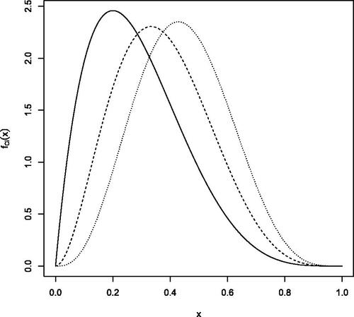
Consider a community gathering n = 400 individuals with three risk profiles. Each participant brings a compound Poisson loss to the pool, where severities obey the beta distribution with mean $a/(a+b)$ and variance $ab/({(a+b)}^2(a+b+1)).$ Precisely,

Group 1 (low risks) with $n_1=0.5n$ individuals, ${\lambda }_1=5\%,$ claim sizes distributed as C₁ obeying the beta distribution with parameters a = 2 and b = 5.

Group 2 (medium risks) with $n_2=0.35n$ individuals, ${\lambda }_2=10\%,$ claim sizes distributed as C₂ obeying the beta distribution with parameters a = 3 and b = 5.

Group 3 (high risks) with $n_3=0.15n$ individuals, ${\lambda }_3=20\%,$ claim sizes distributed as C₃ obeying the beta distribution with parameters a = 4 and b = 5.

The probability density functions of C₁, C₂, and C₃ are displayed in Figure 1. We can see there that the probability mass progressively shifts toward larger values. Participants in Group 3 bring comparatively higher severities compared to participants in Group 2, who in turn bring comparatively higher severities compared to participants in Group 1. Groups are thus ranked in increasing magnitude of both expected frequencies and severities.

Figure 1. Probability Density Functions of the Severities C₁ in Group 1 (Solid Line, —), C₂ in Group 2 (Broken Line, - - -), and C₃ in Group 3 (Dotted Line, $···$).

4.2. Conditional Mean Risk Sharing within the Community

The functions $s\mapsto \mathrm{E}[X_i|S=s]$ are displayed in Figure 2 for each of the three groups. They appear to be increasing so that the risk sharing is Pareto-optimal. We can see there that the contribution paid by a member of Group 3 increases more rapidly compared to the contributions paid by members of Groups 1 and 2, because of the larger size of the losses they bring to the pool.

Figure 2. Respective Contributions $s\mapsto \mathrm{E}[X_i|S=s]$ in Group 1 (Solid Line at the Bottom), Group 2 (Broken Line in the Middle), and Group 3 (Dotted Line at the Top).

Figure 3 shows the probability density function of $\mathrm{E}[X_i|S]$ in each of the three groups. The probability mass at 0, equal to $\text{exp}\hspace{0.17em}(-{\lambda }_{•})=2.3195\times {10}^{-16},$ is not displayed there. The probability density functions are bell-shaped. This is an application of the central limit theorem derived in Denuit and Robert (2021).

Figure 3. Probability Density Functions of the Random Variables $\mathrm{E}[X_i|S]$ in (a) Group 1, (b) and (c) Group 3 Together with the Probability Density Function of the Asymptotic Equivalent $h_i^{\text{reg}}(S)$ (Read Dotted Line).

4.3. Stop-Loss Protection

Let us now determine the retention level w satisfying (2.1(2.1) $$\sum _{i=1}^n{\pi }_i-(1+{\theta }_{\text{SL}})\mathrm{E}\left[{(S-w)}_{+}\right]=w.$$(2.1) ) if provisions π_i are of the form (2.6(2.6) $${\pi }_i=(1+{\theta }_{\mathrm{P}2\mathrm{P}})\mathrm{E}\left[X_i\right],$$(2.6) ) with ${\theta }_{\mathrm{P}2\mathrm{P}}=0.2$ and ${\theta }_{\text{SL}}=0.1.$ Figure 4 displays the function $w\mapsto w+{\pi }_{\text{SL}}(w)$ as well as the horizontal line at $(1+{\theta }_{\mathrm{P}2\mathrm{P}})\mathrm{E}[S].$ We can see there that there is a unique crossing corresponding to the retention w of the pool. With the retention w determined in this way, the probability that the cash-back operates is $F_S(w)=84.03\%.$

Figure 4. Function $w\mapsto w+{\pi }_{\text{SL}}(w)$ (Solid Line) and horizontal (Broken) Line at $(1+{\theta }_{\mathrm{P}2\mathrm{P}})\mathrm{E}[S]$ Defining The Retention Level w.

Alternatively, the organizer could also specify the probability (β, say) that there remains some surplus to be shared among the participants, by taking w such that $w=F_S^{-1}(\beta ).$ The corresponding loading ${\theta }_{\mathrm{P}2\mathrm{P}}$ is then given by $${\theta }_{\mathrm{P}2\mathrm{P}}=\frac{F_S^{-1}(\beta )+{\pi }_{\text{SL}}(F_S^{-1}(\beta ))}{\mathrm{E}\left[S\right]}-1.$$

Figure 5 displays the resulting value for ${\theta }_{\mathrm{P}2\mathrm{P}}$ for $\beta \in [50\%,90\%].$ As expected, ${\theta }_{\mathrm{P}2\mathrm{P}}$ increases with β but it remains within an acceptable range.

Figure 5. Loading ${\theta }_{\mathrm{P}2\mathrm{P}}$ Corresponding to the Probability β That a Bonus Can Be Awarded to Participants.

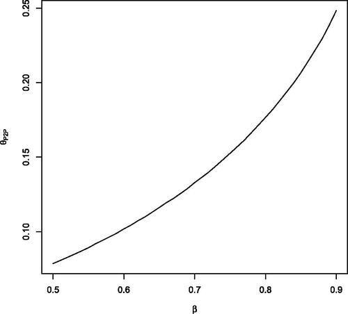
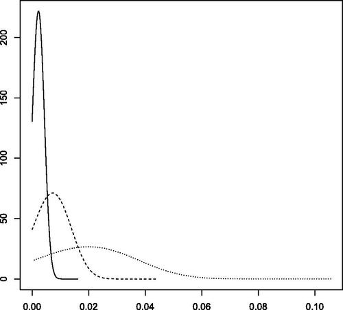
Figure 6. Probability Density Functions of the Cash-Back, Given That $S\le w,$ in Group 1 (Solid Line), Group 2 (Broken Line), and Group 3 (Dotted Line).

4.4. Cash-Backs

Let us now continue with the retention level corresponding to the unique crossing visible in Figure 4, such that $F_S(w)=84.03\%.$ The cash-back mechanism should thus operate on average 4 years out of 5, approximately. Figure 3 shows the probability density function of the bonus $w_i-\mathrm{E}[X_i|S]$ that can be awarded in each of the three groups, given that there is some surplus (that is, given $S\le w).$ The probability mass at 0, equal to $\mathrm{P}[S>w]=15.97\%,$ is not displayed there. We can see in Figure 4 that the probability density functions extend to the right, with comparatively higher bonuses for Groups 2 and 3 in case of a favorable experience.

Given that the conditional mean risk sharing rule does not coincide with $h_1^{\text{prop}},$ there might be some differences between ${\pi }_i^{\mathrm{P}2\mathrm{P}}$ and w_i at an individual level. To see this, let us rewrite ${\pi }_i^{\mathrm{P}2\mathrm{P}}$ as $$\begin{array}{c}{\pi }_i^{\mathrm{P}2\mathrm{P}}=(1+{\theta }_{\mathrm{P}2\mathrm{P}})\mathrm{E}\left[X_i\right]-(1+{\theta }_{\text{SL}})\mathrm{E}\left[{(\mathrm{E}[X_i\left|S\right]-w_i)}_{+}\right]\\ =({\theta }_{\mathrm{P}2\mathrm{P}}-{\theta }_{\text{SL}})\mathrm{E}\left[X_i\right]+(1+{\theta }_{\text{SL}})(\mathrm{E}[X_i]-\mathrm{E}[{(\mathrm{E}[X_i\left|S\right]-w_i)}_{+}])\\ =({\theta }_{\mathrm{P}2\mathrm{P}}-{\theta }_{\text{SL}})\mathrm{E}\left[X_i\right]+(1+{\theta }_{\text{SL}})\mathrm{E}\left[\min \right\{\mathrm{E}\left[X_i\right|S],w_i\}].\end{array}$$

In our example, these differences materialize into the values of w_i respectively equal to 0.01616265, 0.04364075, and 0.1056294 in Groups 1, 2, and 3, whereas the corresponding values of ${\pi }_i^{\mathrm{P}2\mathrm{P}}$ are 0.01665736, 0.0437729, and 0.1037132. Thus, ${\pi }_i^{\mathrm{P}2\mathrm{P}}>w_i$ in Groups 1 and 2 whereas the reverse inequality holds in Group 3.

The differences between w_i and ${\pi }_i^{\mathrm{P}2\mathrm{P}}$ at an individual level remain rather small but they induce some transfers between groups. In order to obtain equality—that is, to restore fairness we can use the large-pool approximation to the conditional mean risk sharing $\mathrm{E}[X_i|S]$ and replace the premium calculation principle for π_i by the variance principle, as explained next.

4.5. Large-Pool Approximation

Let ${\sigma }_i^2=\text{Var}[X_i]$ be the variance of the loss for participant i. When the number of participants is large, Denuit and Robert (2021) established that the linear regression rule allocating $$h_i^{\text{reg}}(S)={\mu }_i+\frac{{\sigma }_i^2}{\sum _{j=1}^n{\sigma }_j^2}\left(S-\mathrm{E}\left[S\right]\right)$$ to participant i, $i=1,2,\dots ,n,$ provides a good approximation to the conditional mean risk sharing rule for compound Poisson losses. Precisely, Denuit and Robert (2021) established that the linear regression sharing rule and the conditional mean sharing rule are asymptotically equivalent, in the sense that the fluctuations of the individual contributions around the pure premium are roughly identical when n becomes large enough. Given that both risk sharing rules converge to μ_i with probability 1, the linear regression rule provides a reasonable approximation to the conditional mean risk sharing rule when the size of the pool becomes large. The probability density function of the asymptotically equivalent linear rule $h_i^{\text{reg}}(S)$ is also represented Figure 3. It appears to be almost identical to the true density, showing that the quality of the linear approximation $h_i^{\text{reg}}(S)$ to $\mathrm{E}[X_i|S]$ is excellent in this example.

Because the conditional expectations have been assumed to be comonotonic, the approximation also applies to the random vector $(\mathrm{E}[X_1|S],\dots ,\mathrm{E}[X_n|S]);$ that is, we can replace it with $(h_1^{\text{reg}}(S),\dots ,h_n^{\text{reg}}(S))$ to perform the calculations. This provides us with an effective way to make the system actuarially fair in large pools; that is, to ensure that the identity ${\pi }_i^{\mathrm{P}2\mathrm{P}}=w_i$ holds for all i.

Precisely, let us replace formula (2.6(2.6) $${\pi }_i=(1+{\theta }_{\mathrm{P}2\mathrm{P}})\mathrm{E}\left[X_i\right],$$(2.6) ) with provisions computed according to the variance premium calculation principle; that is, $${\pi }_i=\mathrm{E}\left[X_i\right]+{\theta }_{\mathrm{P}2\mathrm{P}}\text{Var}\left[X_i\right]=\mathrm{E}\left[X_i\right]+{\theta }_{\mathrm{P}2\mathrm{P}}\text{Cov}[X_i,S].$$

The retention of the pool is still obtained as the solution to (2.1(2.1) $$\sum _{i=1}^n{\pi }_i-(1+{\theta }_{\text{SL}})\mathrm{E}\left[{(S-w)}_{+}\right]=w.$$(2.1) ) so that w is such that ${\sum }_{i=1}^n{\pi }_i-{\pi }_{\text{SL}}=w$ with the same ${\pi }_{\text{SL}}$ and ${\pi }_i^{\text{SL}}$ as before. Let us now establish that the desired equality ${\pi }_i^{\mathrm{P}2\mathrm{P}}=w_i$ holds for all i. Starting from $$\begin{array}{c}{w}_i=F_{h_i^{\text{reg}}(S)}^{-1}(F_S(w))\\ =\mathrm{E}\left[X_i\right]+\frac{\text{Var}\left[X_i\right]}{\text{Var}\left[S\right]}(w-\mathrm{E}[S])\\ =\mathrm{E}\left[X_i\right]+\frac{\text{Var}\left[X_i\right]}{\text{Var}\left[S\right]}(\mathrm{E}[S]+{\theta }_{\mathrm{P}2\mathrm{P}}\text{Var}[S]-(1+{\theta }_{\text{SL}})\mathrm{E}[{(S-w)}_{+}]-\mathrm{E}[S])\\ =\mathrm{E}\left[X_i\right]+{\theta }_{\mathrm{P}2\mathrm{P}}\text{Var}\left[X_i\right]-(1+{\theta }_{\text{SL}})\frac{\text{Var}\left[X_i\right]}{\text{Var}\left[S\right]}\mathrm{E}\left[{(S-w)}_{+}\right]\end{array}$$ and noting that $$\frac{\text{Var}\left[X_i\right]}{\text{Var}\left[S\right]}\mathrm{E}\left[{(S-w)}_{+}\right]=\mathrm{E}\left[{\left(\frac{\text{Var}\left[X_i\right]}{\text{Var}\left[S\right]}S-\frac{\text{Var}\left[X_i\right]}{\text{Var}\left[S\right]}w\right)}_{+}\right]=\mathrm{E}\left[{(\mathrm{E}[X_i\left|S\right]-w_i)}_{+}\right],$$ we get $$\begin{array}{c}{w}_i={\pi }_i-(1+{\theta }_{\text{SL}})\mathrm{E}\left[{(h_i^{\text{reg}}(S)-w_i)}_{+}\right]\\ ={\pi }_i-{\pi }_i^{\text{SL}}\\ ={\pi }_i^{\mathrm{P}2\mathrm{P}}\end{array}$$ so that we conclude that ${\pi }_i^{\mathrm{P}2\mathrm{P}}=w_i$ holds true for every participant.

4.6. Hierarchical Risk Sharing

As an alternative to the individual sharing rule described so far, we could proceed in two steps, by splitting the total losses S among the three groups and then allocating the result among participants within each group. Thus, we decompose the whole community according to two levels, the group level and the individual-within-the-group level, and proceed with the help of the hierarchical risk sharing described in Section 3.

Inside each group j, losses $X_{j,i}$ are identically distributed: They all obey the same compound Poisson distribution with expected frequency λ_j and severities distributed as C_j. The totals S_j are thus also compound Poisson distributed, with expected frequency $n_j{\lambda }_j$ and severities distributed as C_j, $j\in \{1,2,3\}.$ Each group is then allocated the amount $\mathrm{E}[S_j|S]$ whose distribution can be obtained as in the one-step analysis conducted before. In particular, we have $\mathrm{E}[S_j|S=s]=n_j\mathrm{E}[X_{j,1}|S=s]$ where the functions $s\mapsto \mathrm{E}[X_{j,1}|S=s]$ are depicted in Figure 2. Because groups are homogeneous, the total $\mathrm{E}[S_j|S=s]$ is uniformly distributed over members, each of them receiving $\mathrm{E}[S_j|S=s]/n_j,$ which reconciles both approaches.

5. CONCLUSION

In this article, we have designed a collaborative insurance scheme limiting the contributions paid by participants to an initial, ex ante provision calculated by adding a proportional loading to the pure premium (or expected loss). A cash-back mechanism operates ex post, to restore fairness. Because the realization of actual losses X_i is mostly due to chance, revealing only partly the underlying magnitude of the risk brought to the community, the system assigns structural losses $\mathrm{E}[X_i|S]$ to participants, whereas the departures ${\mathcal{E}}_1,{\mathcal{E}}_2,\dots ,{\mathcal{E}}_n$ are reallocated among them according to the mutuality principle. See decomposition (1.1(1.1) $$X_i=\underset{=\text{structural}\mathrm{ }\text{part}}{\underbrace{\mathrm{E}\left[X_i\right|S]}}+\underset{=\text{random}\mathrm{ }\text{departure}\mathrm{ }{\mathcal{E}}_i}{\underbrace{X_i-\mathrm{E}\left[X_i\right|S]}}.$$(1.1) ).

Risk sharing is limited to the lower layer, which acts as a pooled deductible. Within P2P insurance communities, the risk borne by each participant can be determined in proportion to the initial contributions (proportional mean risk sharing). The total risk-bearing capacity for the lower layer is then determined accordingly. Whereas pure P2P insurance does not include any guarantee, the collaborative insurance scheme designed here supplements risk sharing with risk transfer of a higher layer, operated by a (re-)insurer.

To ensure full transparency, it is important to inform participants by issuing regular reports that disclose meaningful indicators. A yearly summary can be issued to policyholders to describe loss experience over the past period and make explicit the amount of risk sharing and risk transfer, listing for participant i actual costs X_i together with the part $\mathrm{E}[X_i|S]$ that can be attributed to participant i individually and the departure ${\mathcal{E}}_i$ mutualized inside the community. All calculations are based on incurred amounts. This is particularly important Because the yearly account must assess the overall costs. All open and incurred but not reported cases at the end of the period are “sold” to the (re-)insurer, which settles them for a given price.

Insurance activities require risk-bearing capital provided by stock holders. The amount of capital required by regulatory authorities is then paid by each policyholder, in a cost-of-capital approach. This burden is avoided for the lower layer but still present for the cover protecting the upper layer. The corresponding premium can be considered as part of running expenses and benefits can be allocated to each policy. If the community also buys excess-of-loss covers, the policy-specific reinsurance premium can be included in the yearly account and the stop-loss premium can be allocated to each participant according to the respective “use” of the upper layer.

The collaborative insurance offer can also broaden the range of risks that can be covered. Traditionally, risks with low severity have been excluded from insurance because administrative and settlement expenses were considered to be too expensive. With automation of the customer relationship and the claim settlement process, this point of view becomes somewhat outdated and this offers a huge potential new market for insurance providers.

In this way, insurers could broaden the range of risks covered to a very large extent, diversifying the offered services and investing in the coverage of small risks that have been so far excluded from insurance policies. Insurance has traditionally been restricted to low frequency–high–severity risks, because of expensive claim handling costs. But nowadays, consumers are ready to pay for peace of mind. Consequently, they also cover small pieces of equipment (like smartphones), pay “premiums” for extended warranty, or buy comprehensive maintenance and assistance contracts (e.g., from energy providers). There is thus a trend towards covering high-frequency–low-severity risks to avoid time-consuming management or to smooth household budgets by paying fixed monthly fees (for instance, medical outpatient insurance coverage). These risks are even easier to model and manage compared to traditional insurance risks, but their coverage requires automated handling and adapted procedures (such as direct repair though a network of carefully selected, continuously assessed and rewarded subcontractors) to be economically feasible. Thus, the approach proposed in this article is effective to expand coverages to smaller risks that are easy to manage through P2P insurance.

Discussions on this article can be submitted until October 1, 2021. The authors reserve the right to reply to any discussion. Please see the Instructions for Authors found online at http://www.tandfonline.com/uaaj for submission instructions.

ACKNOWLEDGMENTS

The authors thank two anonymous referees and a co-editor for their constructive comments, which greatly helped to significantly improve this article.

REFERENCES

- Clemente, G. P., and P. Marano. 2020. The broker model for peer-to-peer insurance: An analysis of its value. The Geneva Papers on Risk and Insurance - Issues and Practice 45: 457–81 doi:https://doi.org/10.1057/s41288-020-00165-8
- Denuit, M. 2019. Size-biased transform and conditional mean risk sharing, with application to P2P insurance and tontines. ASTIN Bulletin 49:591–617.
- Denuit, M. 2020a. Investing in your own and peers’ risks: The simple analytics of P2P insurance. European Actuarial Journal 10:335–59. doi:https://doi.org/10.1007/s13385-020-00238-x
- Denuit, M. 2020b. Size-biased risk measures of compound sums. North American Actuarial Journal 24: 512–32 doi:https://doi.org/10.1080/10920277.2019.1676787
- Denuit, M., and J. Dhaene. 2012. Convex order and comonotonic conditional mean risk sharing. Insurance: Mathematics and Economics 51:265–70. doi:https://doi.org/10.1016/j.insmatheco.2012.04.005
- Denuit, M., and C. Y. Robert. 2020a. Efron’s asymptotic monotonicity property in the Gaussian stable domain of attraction. Submitted. https://dial.uclouvain.be/pr/boreal/object/boreal:232135
- Denuit, M., and C. Y. Robert. 2020b. Large-loss behavior of conditional mean risk sharing. ASTIN Bulletin 50:1093–122. doi:https://doi.org/10.1017/asb.2020.23
- Denuit, M., and C. Y. Robert. 2021. From risk sharing to pure premium for a large number of heterogeneous losses. Insurance: Mathematics and Economics 96: 116–26. doi:https://doi.org/10.1016/j.insmatheco.2020.11.006
- Dhaene, J., M. Denuit, M. J. Goovaerts, R. Kaas, and D. Vyncke. 2002a. The concept of comonotonicity in actuarial science and finance: Applications. Insurance: Mathematics and Economics 31:133–61. doi:https://doi.org/10.1016/S0167-6687(02)00135-X
- Dhaene, J., M. Denuit, M. J. Goovaerts, R. Kaas, and D. Vyncke. 2002b. The concept of comonotonicity in actuarial science and finance: Theory. Insurance: Mathematics and Economics 31:3–33.
- Efron, B. 1965. Increasing properties of Polya frequency function. The Annals of Mathematical Statistics 36:272–79. doi:https://doi.org/10.1214/aoms/1177700288
- Furman, E., A. Kuznetsov, and R. Zitikis. 2018. Weighted risk capital allocations in the presence of systematic risk. Insurance: Mathematics and Economics 79:75–81.
- Shaked, M., M. A. Sordo, and A. Suarez-Llorens. 2012. Global dependence stochastic orders. Methodology and Computing in Applied Probability 14:617–48. doi:https://doi.org/10.1007/s11009-011-9253-8