Short- and Long-Term Dynamics of Cause-Specific Mortality Rates Using Cointegration Analysis

Abstract

This article applies cointegration analysis and vector error correction models to model the short- and long-run relationships between cause-specific mortality rates. We work with the data from five developed countries (the United States, Japan, France, England and Wales, and Australia) and split the mortality rates into five main causes of death (infectious and parasitic, cancer, circulatory diseases, respiratory diseases, and external causes). We successively adopt short- and long-term perspectives, and analyze how each cause-specific mortality rate impacts and reacts to the shocks received from the rest of the causes. We observe that the cause-specific mortality rates are closely linked to each other, apart from the external causes that show an entirely independent behavior and hence could be considered as truly exogenous. We summarize our findings with the aim to help practitioners set more informed assumptions concerning the future development of mortality.

1. INTRODUCTION

It is commonly known that mortality rates have been decreasing for many decades. Although a joyful development per se, these changes pose serious problems for insurance companies, pension funds, and social security schemes, because they need to know whether the observed decline will continue, slow down, or, speed up. In this work, we will not venture to forecast the prospective evolution of mortality rates but provide new insights on past developments. We believe that once we better understand the past, we will be able to make better prognoses about the future.

Numerous parametric models have been developed in order to take into account characteristics of mortality rate development such as age, year of birth, and rate of improvement. For a review thereof we direct the interested reader to Booth and Tickle (2008), Cairns (2013) and Debón, Montes, and Sala (2006) and references therein. For our part, we want to gain additional insight into the past development of mortality rates by concentrating on a more detailed breakdown of mortality data, namely, by causes of death. Indeed, just from an eye inspection of the cause-specific mortality rates, it becomes clear that these rates showed strikingly divergent trends over the last 50 to 60 years. These phenomena have already been extensively studied and described (e.g., Himes 1994; Horiuchi and Wilmoth 1997; Costa 2005; Cutler, Deaton, and Lleras-Muney 2006).

However, it is much more difficult to integrate cause-specific mortality rates into a model, because they are dependent, and this dependence is, strictly speaking, not observable. Indeed, given a death event at a young age from an accident, for example, it is impossible to say what the chances of this person would be to die later from cancer or any other cause, had he or she remained alive. Among theories and methods trying to take into account the dependency structure between the cause-specific mortality rates one can cite models incorporating individual risk factors (e.g., Manton and Poss 1979; Manton, Stallard, and Trolley 1991), models employing multiple cause-of-death data (e.g., Manton and Myers 1987; Mackenbach et al. 1999); and, more recently, copulas (e.g., Lo and Wilke 2010; Dimitrova, Haberman, and Kaishev 2013).

Although possible theoretically, models that take into account the dependency between the causes of death are problematic to use in practice, because they require a significant amount of additional data that are not readily available. For this reason, the most widely used approach is still based on the assumption of independence between the causes of death that was developed more than 50 years ago (Chiang 1968). In this study, we want to look at the connections between the causes from a different angle. Without trying to describe exactly the dependency structure between the rates of death, we propose an approach based on cointegration analysis that complements the methods and practices mentioned above. In a nutshell, two nonstationary time series are said to be cointegrated if there exists such a linear combination of them that is stationary. Consequently, these time series are linked to each other in the long run and are subject to common stochastic trends. Cointegration analysis thus provides new insights on how cause-specific mortality rates depend from each other and interact in the long run.

Cointegration analysis was first introduced in the seminal paper of Engle and Granger (1987) and received a lot of attention from researchers in the years that followed. Numerous tests allowing one to check for the existence of cointegrated relations between the time variables were developed, and those conceived by Søren Johansen (1988) are among the most widely used. Cointegration analysis and the vector error-correction models (VECMs) based on it quickly became popular in the field of econometrics because they permitted establishing the long-run relationships between variables such as interest rates, consumption, income, etc. (e.g., Baillie and Selover 1987; Clarida 1992; Johansen and Juselius 1992).

To the best of our knowledge, cointegration analysis was first applied to the cause-specific mortality rates in Arnold and Sherris (2013, 2015, 2016). We want to go further and extend the analysis by applying a wider range of cointegration and VECM tools to the cause-of-death mortality rates. We aim to identify new relationships and development patterns that were not covered by the abovementioned authors.

Namely, we want to understand the way the cause-specific mortality rates interact with each other. Using the additional tools offered by the VECMs, we study the short- and long-term impacts that a change in a particular death rate produces in other cause-specific mortality rates. Because we do not have prior knowledge about the precise way the cause-specific mortality rates interact, our study is exploratory in nature and provides new insight by observing the historical data from the perspective of cointegration analysis. Indeed, there are multiple ways in which the cause-specific mortality rates can impact each other. On the one hand, being subject to the same trends (e.g., improving health care systems, changes in nutrition and lifestyle), the cause-specific mortality rates can show similar responses and thus, be positively correlated. On the other hand, because of the presence of competing risks, the reduction in one cause-specific mortality rate will necessarily and at least partially be compensated by increase in other causes and thus, the cause-specific mortality rates will show negative correlation. In absence of a theoretical model for the relations between the causes, we think that the data analysis can reveal the end sum of such interactions.

At the same time, once a certain pattern is revealed in one country, it is impossible to say whether this pattern is a reflection of that country’s particularities or corresponds to some more fundamental processes and hence can be generalized to other countries and datasets. For this reason, we start with the gender-specific statistics of deaths by cause from five highly populated countries with similar socioeconomic characteristics and available observation periods (the United States, Japan, France, England and Wales, and Australia). Thanks to this approach, general common patterns are revealed in regard to the interaction existing between the causes of death. At a later point, our analysis could be extended to include other countries as well.

We see multiple ways in which our findings could be used in practice. First, the general patterns revealed by our approach can serve as a theoretical point of comparison for epidemiological studies on the joint development of cause-specific mortality rates due to particular factors; for example air pollution impacting not only respiratory but also circulatory mortality rates (Zmirou et al. 1998); sedentary behavior impacting both circulatory and cancer mortality rates (Matthews et al. 2012); body mass index providing contrasting effects on circulatory and respiratory mortality rates (Breeze et al. 2006); influenza vaccinations reducing all cause-specific mortality rates (Wang et al. 2007); heat waves impacting several cause-specific mortality rates at once (Rey et al. 2007; Basaga ∼ na et al. 2011) etc. In a similar way, results of such comprehensive assessments of cause-specific mortality rates, as the Global Burden of Disease Study (GBD 2013 Mortality and Causes of Death Collaborators 2013), can be confronted with those delivered by our model.

As previously mentioned, copula-based models are capable of taking into account the dependence between the cause-specific mortality rates. In the same time, copulas are, strictly speaking, not identifiable (Tsiatis 1975). For this reason, research articles usually present several copulas and play with different parameter values, because these choices can have a tremendous impact on the projection results (Dimitrova, Haberman, and Kaishev 2013; Li and Lu 2019). Efforts are made to narrow the set of possible parameters (Li and Lu 2019), and the question of how to estimate the correlations between the causes of death remains open (Dimitrova, Haberman, and Kaishev 2013). Our study provides a new basis that can be used to calibrate copula-based models because it shows explicitly the extent to which cause-specific mortality rates depend on each other.

Additionally, we contribute to the current discussion regarding whether a cause of death should be considered as endogenous or exogenous. In Arnold and Sherris (2016), the authors observed that the results of the cointegration analysis paralleled the classification used by biologists and demographers between the exogenous and endogenous causes of death. Although this classification is not univocal, under the exogenous causes of death most researchers understand diverse external or environmental factors that cause death and the endogenous causes of death correspond to biological forces that lead to death (Carnes et al. 2006; Arnold and Sherris 2016). Because different views exist on this topic (Carnes and Olshansky 1997), we bring the discussion forward by showing that only the external causes can be classified as entirely exogenous, whereas this is not the case for the infectious and parasitic diseases.

We summarize our findings in a comprehensive form with the objective to help practitioners set more informed assumptions when designing scenarios of the possible future evolution of mortality by cause.

The article is organized as follows: In Section 2 we briefly present the data preparation process along with some theoretical notions of the cointegration analysis. Results from the impulse response analysis and short- and long-term dynamics of the cause-specific mortality rates are then presented in Section 3. Section 4 concludes.

2. DATA AND THE COINTEGRATION FRAMEWORK

2.1. Preparing the Data

We obtained the data for the present study from the WHO Mortality Database (World Health Organization [WHO] 2016), which contains the midyear population and the death numbers by country, year, sex, age group and cause of death as far back as 1950. Five developed countries were chosen for the analysis: the United States, Japan, France, England and Wales, and Australia (US, JP, FR, E&W, and AU, respectively).

To ensure consistency between the countries, the WHO defines the causes of death according to the International Classification of Diseases (ICD). This classification changed three times since the inception of the database, switching from ICD-7 to ICD-10 to account for advances in medical science and to refine the classification. We split the causes of death under each classification into five main groups: infectious and parasitic diseases (I&P), cancer, diseases of the circulatory system, diseases of the respiratory system, and external causes (Table 1). These groups account for approximately 70% to 80% of deaths in recent years and made up approximately 50% to 70% of deaths at the onset of the observations.

TABLE 1 Five Main Groups of Causes of Death According to Different Versions of the International Classification of Diseases

Causes of death	ICD 7	ICD 8	ICD 9	ICD 10
I&P	001–138	001–136	001–139	A00–B99
Cancer	140–239	140–239	140–239	C00–D48
Circulatory	400–468	390–458	390–437	I00–I99
Respiratory	470–527	460–519	460–519	J00–J98
External	E810–E999	E810–E999	E800–E999	V00–Y89

The data are divided into the following age groups: deaths at 0, 1, 2, 3, and 4 years and, then into five-year age groups: 5 to 9 years, …, 90 to 94 years, and 95 years and above. Having created two new age groups by grouping together the ages from 1 to 4 as well as 85 and above, we obtained the cause-specific mortality rates by the following transformations:

1. Grouping the death numbers according to the five causal categories.

2. Distributing the number of deaths at unspecified ages proportionally among known age groups.

3. Calculating simple mortality rates as the number of deaths by age, sex, and cause of death divided by the mid-year population by age and sex: $$m_{x,t,d,s,c}=d_{x,t,d,s,c}/l_{x,t,s,c},$$ where $d_{x,t,d,s,c}\text{is}\mathrm{}\text{the}\mathrm{}\mathrm{}\text{number}\mathrm{}\text{of}\mathrm{}\text{deaths}\mathrm{}\text{at}\mathrm{}\text{age}\mathrm{}x,\mathrm{}\text{in}\mathrm{}\text{year}\mathrm{}t,\mathrm{}\text{for}\mathrm{}\text{cause}\mathrm{}\text{of}\mathrm{}\text{death}\mathrm{}d,\mathrm{}\text{gender}\mathrm{}s\mathrm{}\text{and}\mathrm{}\text{country}\mathrm{}c\text{;}{l}_{x,t,s,c}\text{is}\text{the}\mathrm{}\text{mid}-\text{year}\mathrm{}\text{population}\mathrm{}\text{at}\mathrm{}\text{age}\mathrm{}x,\mathrm{}\text{in}\mathrm{}\text{year}\mathrm{}t,\mathrm{}\text{gender}\mathrm{}s,\mathrm{}\text{and}\mathrm{}\text{country}\mathrm{}c;\text{and}{m}_{x,t,d,s,c}\text{is}\mathrm{}\text{the}\mathrm{}\text{central}\mathrm{}\text{death}\mathrm{}\text{rate}\mathrm{}\text{at}\mathrm{}\text{age}\mathrm{}x,\text{in}\mathrm{}\text{year}\mathrm{}t,\mathrm{}\text{for}\mathrm{}\text{cause}\mathrm{}\text{of}\mathrm{}\text{death}\mathrm{}d,\mathrm{}\text{gender}\mathrm{}s,\mathrm{}\text{and}\mathrm{}\text{country}\mathrm{}c.$

4. Applying the comparability ratios to ensure that the observations under the different versions of the ICD are comparable. A comparability ratio is defined in such a way that the average of the mortality rates over the last 2 years of a classification coincide with the average of the mortality rates over the first 2 years of the next classification. For the whole period under the observation, the mortality rates in a new classification are divided by the comparability ratios linking this classification with the previous one(s). In this way, we can smooth the mortality rates across the classifications and remove the discontinuities.

5. Calculating the age-standardized central death rates, the standard population being equal to (1) the U.S. male population in 2007 and (2) the Japanese female population in 2009. In this manner, we ensure that the age structure of the population is the same for all countries and does not change over time. By using one relatively young (United States) and one relatively old (Japan) reference population, we can analyze whether the population age structure has an impact on the behavior of the cause-specific mortality rates. In total, we obtain 20 datasets: five countries, two genders, and two population structures.

   The age-standardized death rate $m_{t,d,s,c}^{US}$ in year t for cause d, gender s, and country c, assuming that the population age structure is constant over the whole observation period and is equal to the age structure of the U.S. males population in 2007 is calculated as follows: $$\begin{array}{l}{m}_{t,d,s,c}^{US}=d_{t,d,s,c}^{US}/l_{2007,\mathit{males},\mathit{USA}}\\ d_{t,d,s,c}^{US}=\sum _x{m}_{x,t,d,s,c}\times l_{x,2007,\mathit{males},\mathit{USA}}.\end{array}$$

   The age-standardized death rate $m_{t,d,s,c}^{JP}$ in year t for cause d, gender s, and country c, assuming that the population age structure is constant over the whole observation period and is equal to the age structure of the JP females population in 2009 is calculated as follows: $$\begin{array}{c}{m}_{t,d,s,c}^{JP}=d_{t,d,s,c}^{JP}/l_{2009,\mathit{females},JP}\\ d_{t,d,s,c}^{JP}=\sum _x{m}_{x,t,d,s,c}\times l_{x,2009,\mathit{females},JP}\end{array}$$

   Age-standardized death rates for selected years using the U.S. males population base are shown in Table A1 in the Appendix.

6. Taking the natural logarithm of the death rates. Hereafter we will work with the vector of time series ${\mathbf{y}}_t$ for each gender s, country c, and population age structure $p\in (US,JP):$ $${\mathbf{y}}_{t,s,c}^p=\left(\begin{array}{c}\mathit{log}(m_{t,I\&P,s,c}^p)\\ \mathit{log}(m_{t,\mathit{Cancer},s,c}^p)\\ \mathit{log}(m_{t,\mathit{Circulatory},s,c}^p)\\ \mathit{log}(m_{t,\mathit{Respiratory},s,c}^p)\\ \mathit{log}(m_{t,\mathit{External},s,c}^p)\end{array}\right).$$

   To ease notation, we will sometimes omit the indexes c, s, and p and work with a vector of mortality rates ${\mathbf{y}}_t={(y_{1t},y_{2t},y_{3t},y_{4t},y_{5t})}^T,$ keeping in mind that a separate VECM equation is formulated for each country, sex, and population age structure.

We thus use the same database as in Arnold and Sherris (2016) except for the additional years of observations that we added whenever this was possible (Table 2).

When we started the current study, the WHO database provided the information on the mid-year population for the United States only until 2007, and for unknown reasons the data on Australian numbers of deaths for 2005 were also missing. As a consequence, we were obliged to limit the time series for these two countries to years 2007 and 2004, respectively.

As we will see in the following sections, the conclusions stated in Arnold and Sherris (2016) were reconfirmed using the longer time series for Japan, France, and England and Wales.

TABLE 2 Observation Periods by Country

Country	Arnold and Sherris (2016)	Current study
United States	1950–2007	1950–2007
Japan	1950–2009	1950–2013
France	1952–2008	1952–2011
England and Wales	1950–2009	1950–2013
Australia	1950–2004	1950–2004

2.2. Cointegration Analysis in Application to the Cause-Specific Mortality Rates

As already mentioned, the causes of death are not independent. Cointegration analysis is then a tool that can help to better understand and model the dependence between the cause-specific mortality rates. As introduced in Engle and Granger (1987), the time series ${\mathbf{y}}_t$ that consists of the n nonstationary elements $\left\{y_{it}\right\},$ for $i=1,\dots ,n,$ are said to be cointegrated with a cointegrating vector β if a linear combination $\beta \prime {\mathbf{y}}_t$ is stationary: (1) $${\beta }_1{y}_{1t}+{\beta }_2{y}_{2t}+\dots +{\beta }_n{y}_{nt}=z_t,$$(1) where z_t is a stationary variable of stochastic deviations. In other words, while being non-stationary themselves, the cointegrated time series do not drift too far away from each other; that is there exists a long-run equilibrium relationship between them. In addition, there may be more than one cointegrating vector, so that β becomes a matrix. The variables are then linked to each other by several cointegration relations (CRs), and each relation is linearly independent from the others.

In Arnold and Sherris (2015, 2016) the time series of all cause-specific mortality rates was found to be nonstationary and to have stochastic trends. It was also shown that at least one cointegrating relation existed between the causes of death in each country.

Multivariate dynamic systems of the nonstationary but cointegrated variables can then be modeled using a VECM, an extension of the vector autoregression (VAR) models, which includes not only the time dependency between the variables up to a lag p – 1 but also long-run equilibrium relations between them: (2) $$\Delta {\mathbf{y}}_t=\mathbf{c}+\mathbf{d}t+{\mathbf{\Gamma }}_1\Delta {\mathbf{y}}_{t-1}+{\mathbf{\Gamma }}_2\Delta {\mathbf{y}}_{t-2}+\cdots +{\mathbf{\Gamma }}_{p-1}\Delta {\mathbf{y}}_{t-p+1}+\mathbf{\Pi }{\mathbf{y}}_{t-1}+{ϵ}_t,{}^1$$(2) where $\Delta {\mathbf{y}}_t={\mathbf{y}}_t-{\mathbf{y}}_{t-1}$ denote the first differences of the data time series, c and d are $(n\times 1)$ vectors of constants, ${\mathbf{\Gamma }}_i$ is a $(n\times n)$ matrix of autoregressive coefficients for $i=1,2,\dots ,p-1,$ and $\mathbf{\Pi }{\mathbf{y}}_{t-1}$ represents the cointegrated term. The latter provides the model with the information on the long-run equilibrium between the variables that would otherwise be lost if a VAR model was applied to the differenced variables. The rank of the matrix $\mathbf{\Pi }$ corresponds to the number of cointegration relations.¹

The first differences of the cause-specific mortality rates being stationary² (as verified in Arnold and Sherris 2016), Equation (2)(2) $$\Delta {\mathbf{y}}_t=\mathbf{c}+\mathbf{d}t+{\mathbf{\Gamma }}_1\Delta {\mathbf{y}}_{t-1}+{\mathbf{\Gamma }}_2\Delta {\mathbf{y}}_{t-2}+\cdots +{\mathbf{\Gamma }}_{p-1}\Delta {\mathbf{y}}_{t-p+1}+\mathbf{\Pi }{\mathbf{y}}_{t-1}+{ϵ}_t,{}^1$$(2) will only hold if the term $\mathbf{\Pi }{\mathbf{y}}_{t-1}$ is also stationary; that is, if the variables are cointegrated. Then the $(n\times 1)$ vector ${ϵ}_t$ is a vector of white noise terms³, with (3) $$E({ϵ}_t)=0,$$(3) (4) $$E({ϵ}_t{ϵ}_l)=\{\begin{array}{cc}\mathbf{\Omega }\hfill & \text{for}t=l\hfill \\ 0\hfill & \text{for}t\ne l,\hfill \end{array}$$(4) where $\mathbf{\Omega }$ is a symmetric positive definite matrix. More details on the VECM and VAR models can be found in Hamilton (1994) and Lütkepohl (2005).

The number of cointegrating relations, if any, can then be found using the trace and the maximum eigenvalue tests developed by Johansen (1995). The Johansen approach also allows finding the matrix $\mathbf{\Pi }$ as (5) $$\mathbf{\Pi }=\alpha \beta \prime ,$$(5) where β is a (n × r) matrix containing r vectors each representing a CR and α is a (n × r) loading matrix that indicates how a particular variable is impacted by the CR. Under the Johansen approach, we can also test for the form of the deterministic elements. Let ${\mu }_t=\mathbf{c}+\mathbf{d}t$ denote the deterministic part of the model and let $\mathbf{d}=\alpha \rho +{\alpha }_{\perp }\gamma ,$ where $\alpha {\alpha }_{\perp }=0.$ Because the mortality rates are known to have a trend, we will consider the following forms of the deterministic elements (Johansen, 1995):

• NT: no trend in the VECM but a linear trend in the levels of the variables: $\mathbf{c}\ne 0,\rho =0,\gamma =0,\text{hence}\mathbf{d}=0,$

• TC: linear trend in the CR combined with a linear trend in the levels of the variables (i.e., no linear trend in the differenced variables) $\mathbf{c}\ne 0,\rho \ne 0,\gamma =0,\text{hence}\mathbf{d}=\alpha \rho ;$

• QT: linear trend in the differenced variables, thus the quadratic trend in the levels of the variables (i.e., the VAR model) $\mathbf{c}\ne 0,\rho \ne 0,\gamma \ne 0,\text{hence}\mathbf{d}=\alpha \rho +{\alpha }_{\perp }\gamma .$

In the tables that follow we will refer to the abbreviations NT, TC, and QT when describing the form of the deterministic elements chosen for a particular dataset.

Once the coefficients of the VECM model (Equation 2(2) $$\Delta {\mathbf{y}}_t=\mathbf{c}+\mathbf{d}t+{\mathbf{\Gamma }}_1\Delta {\mathbf{y}}_{t-1}+{\mathbf{\Gamma }}_2\Delta {\mathbf{y}}_{t-2}+\cdots +{\mathbf{\Gamma }}_{p-1}\Delta {\mathbf{y}}_{t-p+1}+\mathbf{\Pi }{\mathbf{y}}_{t-1}+{ϵ}_t,{}^1$$(2) ) are defined, they allow us to assess the short- and long-term dynamics of the system. Indeed, the coefficients of the ${\mathbf{\Gamma }}_i$ matrices indicate whether and to what extent the cause-specific mortality rates interact in the short run. On the other hand, the analysis of the coefficients of the matrices α and β provide us with the information on the long-term relationships in the system.

In particular, the Johansen approach can be used to test whether every coefficient in the CR (i.e., in the matrix β) is significantly different from zero. If this is not the case, we can conclude that a particular variable does not participate in the long-run equilibrium. In Arnold and Sherris (2016) it was found that in all countries and at least for one of the sexes the pair of mortality rates corresponding to I&P diseases and external causes did not appear significantly in the long-run equilibrium. The cointegration analysis hence showed that the long-term equilibrium relationship existed only between the mortality rates that could be classified as endogenous causes of death (cancer, circulatory, and respiratory diseases), and exogenous causes (I&P diseases, external causes) were excluded. Interestingly, this result coincides with the distinction used by biologists and demographers between the exogenous and endogenous causes of death. In this article, we will complement this study by analyzing first the short-term component and, second, the matrix α; that is, the impact that the CR has on a particular mortality rate.

2.3. Introducing the Lag of 2 to the VECM Setup

A usual step when working with a VECM setup is to define the lag order to be used in the VECM or the corresponding VAR model. Although in Although in Arnold and Sherris (2016) the VAR models with the lag order of one were indicated as optimal using Akaike’s information criterion, Hannan-Quinn criterion, Schwarz criterion, and final prediction error⁴ for some of the datasets, the corresponding model cannot be used to answer our research question. Indeed, in this case the VECM equation has no lagged values; consists only of the CR, errors, and eventual deterministic terms and implies that there is no connection between the first differences of the cause-specific mortality rates in the short run: (6) $$\Delta {\mathbf{y}}_t=\mathbf{c}+\mathbf{dt}+\mathbf{\Pi }{\mathbf{y}}_{t-1}+{ϵ}_t.$$(6)

Hence, in our case we need a VAR model with a lag order of at least two in order to have a full range of parameters in the VECM. Therefore, as a preliminary step, we decide to allow for the presence of the ${\mathbf{\Gamma }}_1\Delta {\mathbf{y}}_{t-1}$ term on the right-hand side of the equation. This gives us the possibility to study the relative importance as well as the significance of the coefficients of the corresponding parameter matrix ${\mathbf{\Gamma }}_1.$ Should some of the matrix ${\mathbf{\Gamma }}_1$ coefficients turn out to be significantly different from 0, we will be able to analyze the short-run adjustments of the cause-specific mortality rates.

The models that were chosen as best describing the datasets in Arnold and Sherris (2016) comprising the VAR(2) models for some of the countries. To be able to make the full analysis of the short-run adjustments, we check whereas for every dataset we can find models with the lag order of two that would suitably describe the data.

First, we apply the Johansen approach to define the number of cointegration relations and the form of the deterministic elements and then we test the residuals of the fitted VECM. The models suggested by the Johansen approach are shown in the Tables A2 to A5 of the Appendix (second column). These are the models that will be used in the subsequent analysis of the short- and long-term dynamics of the cause-specific mortality rates. Further columns contain the results of the tests on the residuals of the fitted VECM. The overall fit is similar to that of the models proposed in Arnold and Sherris (2016) except for the lower fit for the Japanese datasets. In addition, it was not possible to find any suitable VAR(2) model for the E&W females with the JP females population structure, so in the following sections we will use 19 datasets instead of 20.

TABLE 5 Impulse Response Analysis: Response of the Mortality Rate Y to the Shock Given to the Cause X, High-Level Summary across All Countries, Sexes, and Population Structures

X \ Y	I&P	Cancer	Circulatory	Respiratory	External
I&P		Low	Low	Low	Low
Cancer	High		Med	High	High
Circulatory	High	Low		High	Med
Respiratory	Med	Low	Low		Low
External	High	Low	Low	High

For these new models, we also need to check the significance of the β matrix coefficients. As we can see in Tables 3 and 4, for 15 out of 19 considered datasets the cause-specific mortality rates corresponding to the causes I&P and external do not appear significant (at a 1% significance level) in the long-term steady states, which confirms the conclusion made in Arnold and Sherris (2016).

TABLE 3 p Values for the Null Hypothesis That the I&P and the External Causes of Death Are Not Significantly Different from Zero, U.S. Males Population Base, VAR(2) Models

Country	Model	Males	Females
US	VAR(2), QT, 1 CR	0.0655	0.0007
JP	VAR(2), TC, 2 CR	0.4878	0.0810
FR	VAR(2), NT, 1 CR	0.1945	–
	VAR(2), QT, 1 CR	–	0.0062
E&W	VAR(2), QT, 1 CR	0.1607	0.0015
AU	VAR(2), NT, 1 CR	–	0.0438
	VAR(2), QT, 1 CR	0.2570	–

Note: A null hypothesis is accepted at an $\alpha \%$ significance level when the p value is higher than $\alpha \%.$

QT = quadratic trend in the VAR; TC = linear trend in the cointegration relation; NT = no trend; CR = cointegration relation.

TABLE 4 p Values for the Null Hypothesis That the I&P and the External Causes of Death Are Not Significantly Different from Zero, Japanese Females Population Base, VAR(2) Models

Country	Model	Males	Females
US	VAR(2), QT, 1 CR	0.0173	0.0000
JP	VAR(2), QT, 1 CR	0.0530	0.1906
FR	VAR(2), NT, 1 CR	0.0999	0.0696
E&W	VAR(2), QT, 1 CR	0.0788	No model
AU	VAR(2), NT, 1 CR	0.1917	—
	VAR(2), QT, 1 CR	—	0.0691

Note: A null hypothesis is accepted at a an $\alpha \%$ significance level when the p value is higher than $\alpha \%.$

As already mentioned, the VAR(2) models indicated in Tables 3 and 4 will be used in the analysis that follows in Section 3.

3. DYNAMICS OF THE CAUSE-SPECIFIC MORTALITY RATES

In the following sections, we present detailed analysis for the two datasets U.S. and Japanese males using the U.S. males population structure. We summarize the most interesting findings and provide the details in the Appendix for the remaining 17 datasets.

3.1. Impulse-Response Analysis

First, to get a high-level overview of interactions between the cause-specific mortality rates (as described by the VECM equations in the preceding section), we apply the framework of impulse response analysis (see, e.g., Lütkepohl 2005,). At this point, we do not differentiate between the short- and long-term elements of the VECM and analyze the system as a whole. More detailed analysis of the short- and long-term components including the statistical significance of the parameters will follow.

Basically, impulse response analysis means that we first give a single shock to one cause-specific mortality rate and then analyze and compare the responses to this shock from every other cause-specific mortality rate. In this way, we study the impact of an unexpected change in a particular mortality rate on the dynamics of the system of mortality rates as observed in the past. The initial value taken by the variable that receives the shock is equal to its own standard deviation.

When analyzing the results, we successively adopt two points of view. First, we compare the impacts that a particular cause induces on other cause-specific mortality rates. Then, we compare the responses of a particular cause to the individual shocks received from the rest of mortality rates. In this way, we are able to determine not only whether a particular cause influences the others and to what extent but also whether it is influenced by the rest of the causes and to what extent.

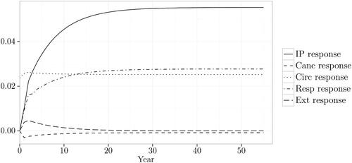
Once a shock is given to a particular cause-specific mortality rate, it propagates in the system and confers new values to the rest of the variables. This development can be suitably exposed on a chart. For example, Figure 1 shows the responses of every cause-specific mortality rate to the shock given to the circulatory mortality rate for U.S. males with the U.S. males population structure (standard deviation of the differenced circulatory mortality rate = 0.0235). Overall, the I&P and respiratory mortality rates show the most important reactions to the shock given to the circulatory mortality rate. The cancer and external mortality rates are insignificantly impacted by the shock given to the circulatory mortality rate. As for the circulatory mortality rate itself, after having received the initial shock, it maintains the increased value until the end of the simulation period.

FIGURE 1. Responses to the Shock Given to the Circulatory Cause, U.S. Males, U.S. Males Population Base.

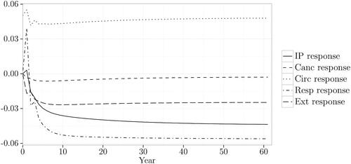
The responses to the shocks from the circulatory cause observed in the dataset for Japanese males with the U.S. males population structure are shown on Figure 2 (standard deviation of the differenced circulatory mortality rate = 0.0501). Similar to the U.S. males dataset, the respiratory cause shows the most important response from the shock given to the circulatory mortality rate. The response of the I&P mortality rate is slightly less important than that of the respiratory rate. Interestingly, both responses have a negative sign, whereas in the U.S. males dataset they also have the same sign but a positive one. One further observation for the Japanese males dataset is that the external causes also show a non-negligible response to the shock from the circulatory cause.

FIGURE 2. Responses to the Shock Given to the Circulatory Cause, Japanese Males, U.S. Males Population Base.

We see that in both cases the system comes rather quickly to a new equilibrium. Because the same observation holds for the rest of the datasets, we will compare the responses following individual shocks at time t = 20 years.

In Figures 1 and 2 the responses are shown in absolute values. However, because the cause-specific mortality rates have different standard deviations, each system receives a shock of a different amplitude. As such, the responses are not comparable between the datasets; that is, a response that would be considered high in one dataset can be considered as medium or low in another dataset. To bring the results to the same comparable basis, we will divide the absolute responses by the standard deviation of the cause-specific mortality rate that receives the shock. Then the response of the respiratory cause to the shock from the circulatory cause; that is the value of the cause-specific respiratory mortality rate at time t = 20 will be expressed as a proportion of the shock received by the system; that is of the standard deviation of the cause-specific circulatory mortality rate.

The results for every dataset are shown in Tables A6 and A7 in the Appendix. For the sake of readability, along with a numerical value we provide a label that indicates whether the response can be considered as low, medium, or high: low if $\left|\mathit{response}\right|<3/8,$ medium if $3/8\le \left|\mathit{response}\right|<7/8,$ and high if $7/8\le \left|\mathit{response}\right|.$ These labels are indicative only and were chosen to provide a roughly equal number of medium and high responses (40% of all responses); the rest are attributed to the category low (60% of all responses). The tables are organized as follows: Each row contains responses of all causes to the shock given to the cause X, and each column contains responses of the cause Y to the shocks from all causes. In this way, we can judge simultaneously whether a particular cause impacts each of the remaining causes and whether it reacts to the shocks received from other causes and to what extent.

TABLE 6 p Values for the Null Hypothesis That α_i Is Not Significantly Different from Zero, U.S. Males Population Structure

Country/sex	Model		$\Delta I{P}_t$	$\Delta \mathit{Can}{c}_t$	$\Delta \mathit{Cir}{c}_t$	$\Delta \mathit{Res}{p}_t$	$\Delta Ex{t}_t$
U.S. males	VAR(2), QT, 1 CR	αi	.000	.085	.243	.001	.496
Japanese males	VAR(2), TC, 2 CR	${\alpha }_{1i}$	.026	.000	.183	.837	.182
		${\alpha }_{2i}$	.000	.001	.500	.000	.836

A synopsis of the observations summarized across the 19 datasets is presented in Table 5.

In a nutshell:

• The I&P and respiratory causes have virtually no impact on all other causes, but show important responses to the shocks received from them.

• The cancer and circulatory mortality rates have an important impact on other causes, especially on the I&P and respiratory mortality rates, but show little response to the shocks from other causes.

• The external causes have an equivocal behavior. On the one hand, they have almost no impact on the cancer and circulatory causes but importantly impact the I&P and respiratory causes. On the other hand, they are not impacted by the I&P and respiratory causes but show important responses to the shocks from the cancer and circulatory causes.

This first analysis shows that the cause-specific mortality rates show different behaviors. At the same time, when a system is analyzed as a whole, many effects are necessarily blended. Therefore, we need to decompose our analysis by separately assessing the short- and long-term dynamics of the system of the mortality rates in order to understand better how the causes of death are related to each other. In the following subsections, we will see what drivers in particular lie behind the observed development of the cause-specific mortality rates.

3.2. Short-Term Dynamics

Once the VECM equations are estimated for each dataset, we can use them to separate the short-term adjustments from the long-term dynamics for each cause-specific mortality rate. Indeed, if a particular coefficient ${\gamma }_{ij}$ of matrix ${\mathbf{\Gamma }}_1$ is significant, then the cause i is influenced by the cause j in the short run. We calculate the standard deviations and the corresponding t-ratios of the estimates as shown in Lütkepohl, 2005).

We start with the dataset for U.S. males with the U.S. males population structure. In the preceding section the following model was chosen as best describing this dataset: $$\begin{array}{l}\Delta {\mathbf{y}}_t=\mathbf{c}+\mathbf{dt}+{\Gamma }_{\mathit{1}}\Delta {\mathbf{y}}_{t-1}+\Pi {\mathbf{y}}_{t-1}+{ϵ}_t\\ \begin{array}{cc}\hfill & =\left[\begin{array}{c}-\mathbf{2}.\mathbf{7}\mathbf{7}\mathbf{1}\mathbf{6}\\ -0.1500\\ -0.2428\\ -\mathbf{2}.\mathbf{0}\mathbf{5}\mathbf{7}\mathbf{3}\\ 0.1558\end{array}\right]+\left[\begin{array}{c}\mathbf{0}.\mathbf{0}\mathbf{0}\mathbf{9}\mathbf{6}\\ 0.0000\\ 0.0000\\ \mathbf{0}.\mathbf{0}\mathbf{0}\mathbf{5}\mathbf{0}\\ 0.0000\end{array}\right]\mathbf{t}+\left[\begin{array}{ccccc}-0.1212& -0.7074& -0.1879& 0.1743& 0.3232\\ -0.0036& 0.0150& -\mathbf{0}.\mathbf{1}\mathbf{6}\mathbf{5}\mathbf{9}& -0.0082& \mathbf{0}.\mathbf{1}\mathbf{3}\mathbf{2}\mathbf{9}\\ -0.0429& -0.1211& 0.0337& -0.0892& 0.1963\\ -0.1345& -0.2944& -0.0850& -\mathbf{0}.\mathbf{3}\mathbf{8}\mathbf{1}\mathbf{0}& \mathbf{1}.\mathbf{1}\mathbf{1}\mathbf{8}\mathbf{9}\\ 0.0416& -0.3232& 0.1981& -\mathbf{0}.\mathbf{1}\mathbf{4}\mathbf{5}\mathbf{5}& 0.2267\end{array}\right]\Delta {\mathbf{y}}_{t-1}\hfill \end{array}\\ +\left[\begin{array}{c}-0.0331\\ -0.0020\\ -0.0030\\ -0.0257\\ 0.0019\end{array}\right]\left[\begin{array}{ccccc}1.7716& -5.4985& -18.6015& 13.2167& 14.1321\end{array}\right]{\mathbf{y}}_{t-1}+{\mathit{ϵ}}_t.\end{array}$$

The significant coefficients are in bold with the selected significance level of 5%. Though many of the ${\mathbf{\Gamma }}_1$ coefficients are not significant, the cause-specific mortality rates from cancer, respiratory, and external causes are influenced by the lagged values of circulatory and external, respiratory and external, and respiratory causes, respectively. We see that in this dataset three out of five cause-specific mortality rates experience the short-term adjustments from other causes. Hence, it was justified to use the VAR(2) setup and include the lagged values of $\Delta {\mathbf{y}}_t$ into the model. Otherwise, an essential piece of information on the development of the cause-specific mortality rates would not have been accounted for. Another interesting observation is that only the respiratory mortality rate shows the autoregressive feature. In other words, the corresponding cause-specific mortality rate is dependent on the lagged value of itself.

For the dataset of Japanese males with the U.S. males population structure, the chosen VECM has two cointegration relations with a constant and a trend, the latter being restricted to the cointegration term: $$\begin{array}{l}\Delta {\mathbf{y}}_t=\mathbf{c}+{\Gamma }_{\mathit{1}}\Delta {\mathbf{y}}_{t-1}+\alpha \beta \prime ({\mathbf{y}}_{t-1}+(t-1))+{ϵ}_t\\ \begin{array}{cc}\hfill & =\left[\begin{array}{c}0.3960\\ -\mathbf{0}.\mathbf{8}\mathbf{5}\mathbf{3}\mathbf{9}\\ -0.7600\\ -1.8252\\ -0.7695\end{array}\right]+\left[\begin{array}{ccccc}-0.1679& 0.5510& 0.1982& 0.0335& 0.2440\\ 0.0143& -\mathbf{0}.\mathbf{3}\mathbf{8}\mathbf{1}\mathbf{8}& -0.0268& 0.0184& 0.0406\\ 0.1343& 0.7531& 0.1711& -\mathbf{0}.\mathbf{1}\mathbf{6}\mathbf{9}\mathbf{2}& 0.0055\\ 0.1477& 2.1179& \mathbf{1}.\mathbf{3}\mathbf{1}\mathbf{0}\mathbf{8}& -\mathbf{0}.\mathbf{5}\mathbf{5}\mathbf{3}\mathbf{7}& -0.1487\\ 0.0307& 0.3048& -0.2898& 0.1305& -0.0906\end{array}\right]\Delta {\mathbf{y}}_{t-1}\hfill \end{array}\\ +\left[\begin{array}{cc}0.0261& 0.3600\\ -0.0186& -0.0425\\ -0.0126& 0.0399\\ 0.0054& 0.8417\\ -0.0154& -0.0149\end{array}\right]\left[\left[\begin{array}{ccccc}1.5951& 7.7055& 0.9876& -1.5822& 1.8454\\ -1.0848& 9.3172& -10.1473& -6.6630& -3.7839\end{array}\right]{\mathbf{y}}_{t-1}+\left[\begin{array}{c}0.1851\\ -0.3817\end{array}\right](t-1)\right]+{\mathit{ϵ}}_t.\end{array}$$ Also for this dataset, many of the ${\mathbf{\Gamma }}_1$ coefficients are not significant. On the other hand, the cause-specific mortality rates corresponding to the causes cancer, circulatory, and respiratory causes, are influenced by the lagged values of the cancer, respiratory, and circulatory and respiratory mortality rates respectively. Again, three out of five cause-specific mortality rates, experience the short-term adjustments from other causes. Therefore, it would not be justified to use the VAR(1) setup for Japanese males with the U.S. males population structure. Similar to the U.S. males dataset, the respiratory cause shows the autoregressive feature, as does the cancer cause.

After the analysis was repeated for the rest of the datasets using both the U.S. males and Japanese females population structures, the results can be summarized as follows:

• In every dataset, there is at least one cause-specific mortality rate that is significantly impacted by other causes in the short run. For this reason, it would not be optimal to use VAR models with the lag order one instead of two.

• Though in the short run the I&P and cancer causes are rarely impacted by other causes, they also infrequently impact the rest of the causes; that is they show a development mostly independent of other causes in the short run.

• On the other hand, the circulatory, respiratory, and external causes are frequently impacted by one or more causes in the short run and also occasionally impact other causes. Hence, these cause-specific mortality rates are more linked in their development to other causes than the I&P and cancer mortality rates are.

• The respiratory cause consistently shows the autoregressive feature. In other words, in many datasets the corresponding cause-specific mortality rate is dependent on the lagged value of itself.

• For all datasets, the larger part of the significant coefficients are negative; that is more often than not the change in the cause-specific mortality rate goes in the opposite direction of the short-term variation of this and/or other cause-specific mortality rates at the previous point in time. More specifically, this means that if the mortality rate of a particular cause of death increases (decreases), the other causes will tend to decrease (increase) in the short run.

A detailed overview of the significant coefficients in ${\mathbf{\Gamma }}_1$ matrix for each dataset is presented in Tables A8 to A11 in the Appendix.

3.3. Long-Term Dynamics

The α matrix allows us to estimate how deviations from the steady-states impact the cause specific mortality rates. For $r=$ 1 (which is the case for the majority of the datasets) we can write the long-term component as follows: $$\begin{array}{c}\mathbf{\Pi }{\mathbf{y}}_{t-1}=\alpha \beta \prime {\mathbf{y}}_{t-1}=\left[\begin{array}{c}{\alpha }_1\\ {\alpha }_2\\ {\alpha }_3\\ {\alpha }_4\\ {\alpha }_5\end{array}\right]\left[\begin{array}{ccccc}{\beta }_1& {\beta }_2& {\beta }_3& {\beta }_4& {\beta }_5\end{array}\right]{\mathbf{y}}_{t-1}\\ =\left[\begin{array}{c}{\alpha }_1\\ {\alpha }_2\\ {\alpha }_3\\ {\alpha }_4\\ {\alpha }_5\end{array}\right]({\beta }_1{y}_{1t-1}+{\beta }_2{y}_{2t-1}+{\beta }_3{y}_{3t-1}+{\beta }_4{y}_{4t-1}+{\beta }_5{y}_{5t-1}).\end{array}$$

This way, if a particular coefficient α_i is significant, the long-term component on the right-hand side of Equation (2)(2) $$\Delta {\mathbf{y}}_t=\mathbf{c}+\mathbf{d}t+{\mathbf{\Gamma }}_1\Delta {\mathbf{y}}_{t-1}+{\mathbf{\Gamma }}_2\Delta {\mathbf{y}}_{t-2}+\cdots +{\mathbf{\Gamma }}_{p-1}\Delta {\mathbf{y}}_{t-p+1}+\mathbf{\Pi }{\mathbf{y}}_{t-1}+{ϵ}_t,{}^1$$(2) is important in explaining the past variations in the corresponding cause-specific mortality rate on the left-hand side. Moreover, the value of this coefficient shows the extent to which the long-term component contributes to the variation in the cause-specific mortality rate in question. As in the previous subsection, we calculated the standard deviations and the corresponding t-ratios of the estimates of α as shown in Lütkepohl (2005). Table 6 shows the p-values for the U.S. males and Japanese males datasets using the U.S. males population structure.

On the one hand, this example shows that for the U.S. males dataset the long-term component enters the equations for the I&P and respiratory mortality rates with a significant coefficient (at a 5% significance level). On the other hand, the equations for cancer, circulatory, and external mortality rates are not significantly impacted by the long-term equilibrium. For Japanese males, there are two long-term components that each enter with a significant coefficient the equations for the I&P and cancer mortality rates; in addition, the second component enters with a significant coefficient the equation for the respiratory mortality rate.

We repeated the analysis for the rest of the datasets, and the results can be summarized as follows:

• The I&P and respiratory causes seem to be the most impacted by the long-term component: The corresponding ${\alpha }_i$ coefficients are significant in 15 out of 19 datasets. A similar observation was made using the framework of the impulse response analysis, because there the I&P and respiratory mortality rates showed an important reaction to the shocks from other causes. Hence, these shocks propagate in the system via the CR(s).

• The external causes seem to be the least impacted: The corresponding ${\alpha }_i$ coefficients are significant in only 5 out of 19 datasets. Interestingly, the results of the impulse response analysis for the external causes were equivocal in that there was an important reaction to the shocks from the cancer and circulatory causes, but a low response to the shocks from the I&P and respiratory causes. The impact from the cancer and circulatory causes may hence come from the short-term adjustments.

• Results for the cancer and circulatory causes are more difficult to interpret: The corresponding ${\alpha }_i$ coefficients are significant in respectively 9 and 11 out of 19 datasets. The results of the impulse response analysis also showed low reactions of the cancer and circulatory mortality rates to the shocks from other causes.

Interestingly, though the I&P and external causes do not participate conjointly in the long-term equilibrium, they show different behaviors when it comes to the impact they experience from this long-term steady state. Indeed, the cointegration relations often enter the equation for the I&P mortality rate with a significant coefficient but seldom have an effect on external causes. Therefore, only the external causes show behavior that is entirely independent from the long-term equilibrium state and, possibly, aging.

An overview of the results for the remaining datasets is shown in Tables A12 and A13 in the Appendix.

3.4. Long-Term versus Short-Term Dynamics

In the previous sections, we have analyzed the short- and long-term elements separately. Now we want to assess the relative importance of the long- and short-run forces. For this purpose, we break down the expected cause-specific mortality rates at time t, based on the information available up to time t–1, in two elements: the short-term (ST) and long-term (LT) components. By comparing the behavior of each of these elements with the realized change in the mortality rates, we assess the relative importance of the long- and short-run forces in terms of their contribution to the variation of the cause-specific mortality rates.

For illustrative purposes, we present the results for the respiratory equation for U.S. males (Figure 3) and the I&P equation for Japanese males (Figure 4), with both datasets using the U.S. males population structure. In the first case, the actual mortality changes fluctuate primarily with the short-term components (the correlation coefficient between $\Delta \mathit{Res}{p}_t$ and LT: 0.268, between $\Delta \mathit{Res}{p}_t$ and ST: 0.336).

FIGURE 3. Respiratory Cause: Actual Mortality Changes, Long- and Short-Term Components (U.S. Males, U.S. Males Population Structure).

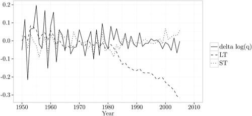
Figure 4. I&P Cause: Actual Mortality Changes, Long-Term and Short Term Components (Japanese Males, U.S. Males Population Structure).

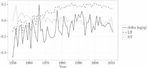
For Japanese males, the actual mortality changes fluctuate primarily with the long-term component (the correlation coefficient between $\Delta I{P}_t$ and LT: 0.570, between $\Delta I{P}_t$ and ST: –0.177).

Because not every equation contains the long-term component, the results for the rest of the datasets are formulated for those cases where the long-term component is present with a significant coefficient ${\alpha }_i.$

• Out of 15 datasets for which the I&P mortality rate equation contains the long-term component, in 13 cases the data fluctuate primarily with the long-term component (i.e., the correlation coefficient between the data points and the long-term component is higher than that between the data points and the short-term component).

• Out of 9 datasets for which the cancer mortality rate equation contains the long-term component, in 8 cases the data fluctuates primarily with the long-term component.

• Out of 11 datasets for which the circulatory mortality rate equation contains the long-term component, in 4 cases the data fluctuate primarily with the long-term component.

• Out of 15 datasets for which the respiratory mortality rate equation contains the long-term component, in 7 cases the data fluctuate primarily with the long-term component.

• Out of 5 datasets for which the External mortality rate equation contains the long-term component, only in 1 case does the data fluctuate primarily with the long-term component.

Summarizing the results stated above, we can say that every time the equation contains the long-term component, the cause-specific mortality rate resembles in its behavior the long-term component rather than the short-term one for the causes I&P and cancer. The opposite is true for the circulatory and external causes. The respiratory mortality rate resembles in its behavior the long-term component as often as it resembles the short-term component.

This observation is not surprising for the I&P and respiratory causes. As we have seen in previous sections, only these cause-specific mortality rates are often impacted by the long-term equilibrium state. At the same time, the I&P mortality rate is rarely impacted and the respiratory mortality rate is frequently impacted by the short-term component. It could have been expected that the I&P mortality rate data will fluctuate with the long-term component in the majority of cases where the I&P mortality rate contains the CR(s). In its turn, the respiratory mortality rate fluctuates either with the short-term component or with the long-term component in roughly similar proportions. Therefore, the correlation analysis reinforces the conclusions of the previous sections for these two rates.

A similar conclusion holds for the circulatory mortality rate: Because it is frequently impacted in the short run and only occasionally in the longrun, the short-term components play a more important role in the correlation analysis.

Regarding the cancer mortality rate, we have seen that it was infrequently impacted by both short- and long-term components. Because none of the effects can be called dominant, the correlation analysis helps to identify the component that plays a more important role in the development of this cause-specific mortality rate, in this case, the long-term.

As for the external causes, the corresponding cause-specific mortality rate is often impacted by the short-term component and virtually never by the long-term one. Even in those rare cases in which the CR enters the equation with a significant coefficient, the data fluctuate more with a short-term component.

The detailed results for each dataset are shown in Tables A14 to A17 in the Appendix.

4. CONCLUSIONS

The analysis of dynamics of the cause-specific mortality rates shows that they are dependent on each other in both short- and long-run. Although the observed experience will never exactly repeat itself in the future, the following observations can help practitioners set more informed assumptions on the future development of mortality rates:

• The common long-run trend shared by the cause-specific mortality rates is contingent on the evolution of the cancer, circulatory, and respiratory mortality rates, because these are the causes that significantly contribute to the CR between the mortality rates.

• Once the common long-run trend is defined, it more heavily impacts the development of the I&P and respiratory mortality rates and to a lesser extent the development of the cancer and circulatory mortality rates. The external causes are exempt from the influence of the common long-term relationship between the causes.

• In the short run, the respiratory mortality rate consistently shows the autoregressive feature.

• Although the short-run dependencies are more challenging to model, they are significantly pronounced in the development pattern of the circulatory, respiratory, and the external mortality rates. In other words, these rates are dependent on each other in the short run.

Coming back to the conclusion made in Arnold and Sherris (2016) that the I&P and external causes do not participate conjointly in the long-term steady state, we see that these causes differ in the way they are impacted by the long-term equilibrium. Though the I&P mortality rate is often impacted by the CR(s) and, when it is, fluctuates more with the long-term component, the external causes show the opposite behavior: The corresponding rate is almost never impacted by the CR(s), and, when it is, it fluctuates more with the short-term component.

We see that the development of the external causes mortality rate is completely independent of the long-term equilibrium in terms of both the contribution to, and influence experienced from the steady state. This is a behavior of what could be called a genuinely exogenous cause of mortality because we observe no long-term impact to or from this cause. It develops in a way that is entirely independent of the observed equilibrium between the rest of the cause-specific mortality rates and is subject to only short-term shocks from other causes. Basically, this observation is not surprising, because under the external causes are grouped causes such as transport and other accidents (falls, poisoning, accidental fire, drowning), suicides, homicides, and war injuries. Therefore, it is rather difficult to imagine a link connecting these mortality rates to the rest of the mortality causes that could be observed over a long time. On the contrary, these causes of mortality can be characterized by randomness and “bad luck” rather than by a steady long-term development.

In turn, the I&P mortality rate does not influence the long-term equilibrium observed between the cause-specific mortality rates but is rather sensitive to the impacts received from this equilibrium. Occasionally, it is also subject to short-term shocks from other causes. We can conclude that though the evolution of the I&P mortality rate does not influence the development of other cause-specific mortality rates—that is a sudden increase or drop in the I&P mortality rate will not affect the rest of the cause-specific mortality rates—its own development depends to a great extent on other causes of death, especially in the long run. Such behavior cannot be described as fully independent, so the I&P cause cannot be classified as a truly exogenous cause in the same way the external causes can.

These observations are consistent with the intuition that the biological processes of aging are reflected in the common stochastic trend shared by the cause-specific mortality rates. Indeed, though it can seem that the infectious or parasitic diseases are similar to the external causes in that the origin of the force affecting the human body lies outside, the underlying biological processes are more complicated, because human beings are not equal when they face an infection. Even during severe epidemics, the probability of getting sick and dying depends to a large extent on the internal immune forces of the individual, which, in turn, depend on, among other factors, age. A well-known example is influenza, which is most dangerous for the elderly. When advancing in age, we are increasingly confronted with competing risks such that a decrease in mortality from circulatory diseases, for example, would leave more vulnerable persons alive who could then die from an infectious disease during an epidemic. It is then understandable that the I&P mortality rate, though not a part of the long-term equilibrium, is substantially affected by it. Our results then confirm and reinforce the link between the cointegration relations observed within a set of cause-specific mortality rates and the biological processes of aging.

One further possible application of the present study is the calibration of copula-based models for the cause-specific mortality rates, which remains an open question. Indeed, because of the indentifiability issue raised by Tsiatis (1975), one usually has to assume that the dependence is represented by a known copula with known parameters. At the same time, copula-based models are highly sensitive with respect to these choices (Dimitrova, Haberman, and Kaishev 2013). As pointed out in Kaishev, Dimitrova, and Haberman (2007), the free parameters could be set according to a priori available (medical) information, about the degree of pairwise dependence between the two competing risks, expressed through Kendall’s τ and/or Spearman’s ρ”. In the absence of additional information and to demonstrate the sensitivity of the results, the authors use four different copulas and five different values of Kendall’s τ, ranging from –0.91 (extreme negative dependence) to 0.91 (extreme positive dependence). In Li and Lu (2019), the authors go further and by introducing hierarchical Archimedean copulas succeed in building a model that allows for different levels of association between the causes of death. For this, they group the causes in different clusters based on the (assumed) level of dependence between the causes, but also admit that the introduced hierarchical structure is not unique. Although our study cannot provide an exact value of parameters to be used in copula-based models, a certain degree of pairwise association (correlation) between the causes of death can be inferred from the results of the impulse response analysis (section 3.1). This could help researchers working with copula-based models further reduce the possible range of free parameters that otherwise have to be chosen arbitrarily. In addition, the revealed differences in the long- and short-term development of the cause-specific mortality rates can serve as the basis for building clusters of the causes.

In the current study, we limited our analysis to the total cause-specific mortality rates and did not differentiate by age. Yet, it is intuitively clear that when analyzed by age the mortality rates will present different development patterns. Because the cause-specific death numbers are available in the WHO database by 5-year age groups, it seems to be a promising path to integrate the age specifics of the mortality rates into the modeling process. However, this remains a challenging task because as, on the one hand, the cointegration tests have been developed for systems with a maximum 12 variables (Osterwald-Lenum 1992) and, on the other, the observation horizon, which goes back as far as 1950, is also rather brief. In our opinion, analysis trying to overcome these difficulties while preserving the information on the age profile has the potential to deliver additional insights on the interaction of the cause-specific mortality rates. Moreover, the biological processes of aging may probably be easier to measure once the data on young ages are excluded from the analysis, because by definition the aging risk factor becomes more important the longer we live. For this reason, the analysis of the cause-specific mortality rates excluding young ages may provide a better measure of the aging process.

Discussions on this article can be submitted until January 1, 2023. The authors reserve the right to reply to any discussion. Please see the Instructions for Authors found online at http://www.tandfonline.com/uaaj for submission instructions.

ACKNOWLEDGMENT

The authors thank an anonymous referee for the useful comments that helped to improve the article. All errors are our responsibility.

FUNDING

Viktoriya Glushko and Séverine Arnold gratefully acknowledge the financial support received from the Swiss National Science Foundation for the project “Cause-Specific Mortality Interactions” (Project Number 100018_162898).

Additional information

Funding

Viktoriya Glushko and Séverine Arnold gratefully acknowledge the financial support received from the Swiss National Science Foundation for the project “Cause-Specific Mortality Interactions” (Project Number 100018_162898)

Notes

1 The corresponding VAR model has p lags: ${\mathbf{y}}_t=\mathbf{c}+\mathbf{d}t+{\xi }_1{\mathbf{y}}_{t-1}+{\xi }_2{\mathbf{y}}_{t-2}+\cdots +{\xi }_p{\mathbf{y}}_{t-p}+{ϵ}_t.$.

2 This observation applies to the studied times series only and should be verified for other countries and time periods.

3 We use the Gaussian setting because this allows us to use the cointegration analysis to model the dependence between the cause-specific mortality rates. Other models such as Poisson autoregression are naturally conceivable and would bring a different and complementary perspective to the analysis when modeling death counts.

4 These criteria are based on the natural logarithm of the determinant of the estimate of the residual covariance matrix ${\widehat{\Sigma }}_{ϵ}=\frac{1}{T}{\sum }_{t=1}^T{\widehat{ϵ}}_t\widehat{ϵ}{\prime }_t,$ where T is the number of observations in the time series, to which a penalty for the number of parameters is added. Though in the general case it is important to pay attention to the parsimony of the model, the weight of the penalty is to some extent arbitrary and can vary depending on the objectives of the study.

APPENDIX

TABLE A.1 Age-Standardized Central Death Rates for Selected Years, U.S. Males Population Base, ×10³

		Females			Males
		1960	1980	2000	1960	1980	2000
US	I&P	0.0852	0.0630	0.1014	0.1888	0.1215	0.1686
	Cancer	1.6269	1.5857	1.5786	2.1394	2.4409	2.2483
	Circulatory	4.3148	2.9428	1.9744	6.8425	5.2315	3.2263
	Respiratory	0.4595	0.3292	0.5124	0.8670	0.8205	0.8512
	External	0.4516	0.3804	0.3058	1.1217	1.0368	0.7731
JP	I&P	0.4350	0.0842	0.0629	0.8160	0.2099	0.1426
	Cancer	1.4299	1.3156	1.1361	2.0147	2.1748	2.1092
	Circulatory	1.6850	1.3904	0.6263	2.2670	1.8094	0.8788
	Respiratory	0.9022	0.3804	0.3551	1.3673	0.6830	0.7941
	External	0.4644	0.3230	0.2476	1.0982	0.7577	0.7161
FR	I&P	0.1759	0.1085	0.0833	0.4487	0.2171	0.1502
	Cancer	1.6852	1.5080	1.3868	2.5972	3.0608	2.8610
	Circulatory	2.1922	1.6042	0.9415	3.3823	2.7013	1.6697
	Respiratory	0.8405	0.3023	0.3385	1.3661	0.6451	0.5930
	External	0.5020	0.5267	0.3623	1.1683	1.1520	0.8470
EW	I&P	0.0721	0.0387	0.0557	0.1764	0.0636	0.0708
	Cancer	1.7114	1.7764	1.5838	2.6498	2.8131	2.2807
	Circulatory	3.7128	2.7551	1.4769	5.7063	4.9203	2.5757
	Respiratory	0.8536	0.9398	0.8048	1.9318	1.8931	1.2785
	External	0.3823	0.3044	0.1780	0.6787	0.5561	0.4205
AU	I&P	0.0695	0.0296	0.0419	0.1518	0.0535	0.0843
	Cancer	1.4781	1.4868	1.4368	2.0721	2.3765	2.1570
	Circulatory	4.0123	3.0032	1.5502	6.5525	5.1796	2.4928
	Respiratory	0.5108	0.4362	0.6109	1.1511	1.1897	1.0071
	External	0.4747	0.4236	0.2625	1.0533	0.9189	0.6118

TABLE A.2 Tests on Residuals of the Fitted VECM, Males, U.S. Males Population Base, VAR(2) Models

		p Value
		Autocorrelation			Normality
Country	Model	15 lags	25 lags	35 lags	Skewness	Kurtosis	Both
US	VAR(2), QT, 1 CR	0.212	0.146	0.181	0.546	0.020	0.066
JP	VAR(2), TC, 2 CR	0.526	0.764	0.810	0.749	0.002	0.015
FR	VAR(2), NT, 1 CR	0.354	0.644	0.824	0.467	0.154	0.244
E&W	VAR(2), QT, 1 CR	0.209	0.146	0.207	0.510	0.558	0.607
AU	VAR(2), QT, 1 CR	0.594	0.297	0.405	0.876	0.002	0.027

Note: QT = quadratic trend in the VAR; TC = linear trend in the cointegration relation; NT = no trend; CR = cointegration relation.

TABLE A.3 Tests on Residuals of the Fitted VECM, Females, U.S. Males Population Base, VAR(2) Models

		p Value
		Autocorrelation			Normality
Country	Model	15 lags	25 lags	35 lags	Skewness	Kurtosis	Both
US	VAR(2), QT, 1 CR	0.133	0.007	0.021	0.768	0.141	0.369
JP	VAR(2), TC, 2 CR	0.539	0.601	0.769	0.007	0.000	0.000
FR	VAR(2), QT, 1 CR	0.066	0.286	0.491	0.420	0.038	0.080
E&W	VAR(2), QT, 1 CR	0.389	0.307	0.353	0.025	0.000	0.000
AU	VAR(2), NT, 1 CR	0.238	0.284	0.262	0.652	0.059	0.175

TABLE A.4 Tests on Residuals of the Fitted VECM, Males, Japanese Females Population Base, VAR(2) Models

		p Value
		Autocorrelation			Normality
Country	Model	15 lags	25 lags	35 lags	Skewness	Kurtosis	Both
US	VAR(2), QT, 1 CR	0.496	0.202	0.202	0.879	0.189	0.511
JPn	VAR(2), QT, 1 CR	0.168	0.103	0.081	0.225	0.047	0.052
FR	VAR(2), NT, 1 CR	0.398	0.615	0.534	0.139	0.009	0.009
E&W	VAR(2), QT, 1 CR	0.225	0.094	0.099	0.722	0.556	0.743
AU	VAR(2), NT, 1 CR	0.521	0.397	0.437	0.407	0.013	0.034

TABLE A.5 Tests on Residuals of the Fitted VECM, Females, Japanese Females Population Base, VAR(2) Models

		p Value
		Autocorrelation			Normality
Country	Model	15 lags	25 lags	35 lags	Skewness	Kurtosis	Both
US	VAR(2), QT, 1 CR	0.168	0.005	0.021	0.123	0.010	0.009
JP	VAR(2), QT, 1 CR	0.469	0.625	0.664	0.000	0.000	0.000
FR	VAR(2), NT, 1 CR	0.096	0.426	0.381	0.324	0.097	0.127
E&W	No suitable VAR(2) model
AU	VAR(2), QT, 1 CR	0.548	0.688	0.353	0.488	0.046	0.108

TABLE A.6 Impulse Response Analysis: Response of the Mortality Rate Y from the Shock Given to the Cause X, U.S. Males Population Base

Cause		Males					Females
X / Y	Country	I&P	Canc	Circ	Resp	Ext	I&P	Canc	Circ	Resp	Ext
I&P	US	0.53 (Med)	–0.01 (Low)	–0.02 (Low)	–0.2 (Low)	0.1 (Low)	–0.05 (Low)	–0.12 (Low)	–0.11 (Low)	–0.47 (Med)	0.24 (Low)
I&P	JP	0.97 (High)	–0.13 (Low)	–0.09 (Low)	–0.12 (Low)	–0.14 (Low)	0.58 (Med)	0.03 (Low)	0.13 (Low)	0.01 (Low)	0.01 (Low)
I&P	FR	1.15 (High)	–0.17 (Low)	–0.07 (Low)	0.38 (Med)	–0.21 (Low)	1.2 (High)	–0.03 (Low)	0.07 (Low)	0.22 (Low)	–0.18 (Low)
I&P	E&W	1.59 (High)	–0.14 (Low)	–0.09 (Low)	–0.33 (Low)	–0.38 (Med)	0.37 (Low)	–0.03 (Low)	–0.08 (Low)	–0.33 (Low)	0.17 (Low)
I&P	AU	0.73 (Med)	0.01 (Low)	–0.02 (Low)	–0.12 (Low)	–0.03 (Low)	–0.1 (Low)	0.01 (Low)	0.16 (Low)	–0.1 (Low)	0.2 (Low)
Canc	US	2.05 (High)	1.13 (High)	–0.15 (Low)	0.75 (Med)	–0.78 (Med)	3.39 (High)	1.64 (High)	–0.61 (Med)	0.8 (Med)	–1.78 (High)
Canc	JP	1.06 (High)	0.24 (Low)	–0.27 (Low)	0.75 (Med)	–0.26 (Low)	4.37 (High)	0.5 (Med)	0.03 (Low)	3.38 (High)	0.98 (High)
Canc	FR	1.46 (High)	0.16 (Low)	–0.92 (High)	0.64 (Med)	–0.86 (Med)	2.27 (High)	0.36 (Low)	0.15 (Low)	4.56 (High)	–0.45 (Med)
Canc	E&W	1.61 (High)	0.58 (Med)	–0.1 (Low)	–2.57 (High)	–1.42 (High)	–4.09 (High)	0.7 (Med)	–0.69 (Med)	–2.96 (High)	0.59 (Med)
Canc	AU	−0.18 (Low)	0.68 (Med)	–0.22 (Low)	–1.33 (High)	–0.37 (Low)	0.97 (High)	0.77 (Med)	–0.01 (Low)	0.57 (Med)	0.03 (Low)
Circ	US	2.26 (High)	–0.04 (Low)	1.07 (High)	1.14 (High)	0.01 (Low)	1.34 (High)	0.05 (Low)	1.42 (High)	1.19 (High)	0.22 (Low)
Circ	JP	−0.79 (Med)	–0.09 (Low)	0.91 (High)	–1.09 (High)	–0.52 (Med)	0.1 (Low)	–0.09 (Low)	0.22 (Low)	–1.03 (High)	–0.61 (Med)
Circ	FR	−1.82 (High)	1.16 (High)	1.96 (High)	–1.23 (High)	1.29 (High)	–0.23 (Low)	0.13 (Low)	0.86 (Med)	–0.51 (Med)	0.17 (Low)
Circ	E&W	0.67 (Med)	–0.11 (Low)	0.69 (Med)	–0.03 (Low)	–0.33 (Low)	0.92 (High)	0.06 (Low)	1.01 (High)	1.04 (High)	–0.2 (Low)
Circ	AU	0.4 (Med)	0.05 (Low)	0.83 (Med)	0.67 (Med)	0.16 (Low)	–0.2 (Low)	0.01 (Low)	0.71 (Med)	–0.7 (Med)	0.01 (Low)
Resp	US	−1.37 (High)	–0.08 (Low)	–0.07 (Low)	0.01 (Low)	0.06 (Low)	–0.77 (Med)	–0.11 (Low)	–0.12 (Low)	0.19 (Low)	–0.01 (Low)
Resp	JP	−0.27 (Low)	0.05 (Low)	–0.05 (Low)	0.15 (Low)	0.07 (Low)	–0.02 (Low)	0.01 (Low)	–0.14 (Low)	0.35 (Low)	0.13 (Low)
Resp	FR	−0.41 (Med)	0.2 (Low)	0.05 (Low)	0.05 (Low)	0.13 (Low)	–0.19 (Low)	0.01 (Low)	–0.08 (Low)	0.19 (Low)	–0.02 (Low)
Resp	E&W	−0.05 (Low)	–0.02 (Low)	–0.05 (Low)	0.53 (Med)	–0.04 (Low)	–0.56 (Med)	–0.03 (Low)	–0.13 (Low)	0.31 (Low)	0.07 (Low)
Resp	AU	−0.34 (Low)	–0.05 (Low)	–0.11 (Low)	–0.02 (Low)	–0.07 (Low)	0.65 (Med)	–0.02 (Low)	–0.16 (Low)	0.84 (Med)	–0.17 (Low)
Ext	US	−4.06 (High)	–0.08 (Low)	0.16 (Low)	–1.01 (High)	1.71 (High)	–3.39 (High)	–0.38 (Med)	–0.16 (Low)	–1.47 (High)	1.38 (High)
Ext	JP	0.42 (Med)	–0.19 (Low)	–0.26 (Low)	–0.32 (Low)	0.68 (Med)	–1.35 (High)	0.16 (Low)	0.58 (Med)	–0.13 (Low)	0.79 (Med)
Ext	FR	0.44 (Med)	–0.28 (Low)	–0.08 (Low)	1.08 (High)	0.63 (Med)	–0.6 (Med)	0.07 (Low)	–0.01 (Low)	0.16 (Low)	1.07 (High)
Ext	E&W	−0.38 (Med)	–0.06 (Low)	–0.05 (Low)	–0.56 (Med)	0.53 (Med)	0.01 (Low)	–0.04 (Low)	–0.05 (Low)	–0.35 (Low)	0.98 (High)
Ext	AU	0.07 (Low)	–0.04 (Low)	0.04 (Low)	0.42 (Med)	0.84 (Med)	–1.1 (High)	0.02 (Low)	0.32 (Low)	–0.16 (Low)	1.05 (High)

TABLE A.7 Impulse Response Analysis: Response of the Mortality Rate Y from the Shock Given to the Cause X, Japanese Females Population Base

Cause		Males					Females
X / Y	Country	I&P	Canc	Circ	Resp	Ext	I&P	Canc	Circ	Resp	Ext
I&P	US	0.41 (Med)	–0.02 (Low)	–0.04 (Low)	–0.21 (Low)	0.09 (Low)	1.25 (High)	0.04 (Low)	–0.07 (Low)	0.16 (Low)	0.03 (Low)
I&P	JP	0.92 (High)	–0.02 (Low)	0.18 (Low)	0.64 (Med)	0.11 (Low)	0.81 (Med)	0 (Low)	0.09 (Low)	0.1 (Low)	0.1 (Low)
I&P	FR	1.07 (High)	–0.17 (Low)	0 (Low)	0.37 (Low)	–0.14 (Low)	1.26 (High)	–0.04 (Low)	–0.14 (Low)	0.37 (Low)	–0.48 (Med)
I&P	E&W	0.78 (Med)	–0.03 (Low)	–0.08 (Low)	0.05 (Low)	0.23 (Low)	No suitable VAR(2) model
I&P	AU	0.3 (Low)	0.03 (Low)	0.08 (Low)	–0.08 (Low)	0.04 (Low)	0.71 (Med)	0.03 (Low)	0 (Low)	0.15 (Low)	–0.02 (Low)
Canc	US	1.22 (High)	1.26 (High)	–0.02 (Low)	0.78 (Med)	–0.48 (Med)	–2.25 (High)	0.94 (High)	–0.8 (Med)	–2.37 (High)	–1.13 (High)
Canc	JP	0.9 (High)	0.95 (High)	0.73 (Med)	2 (High)	0.79 (Med)	0.46 (Med)	0.99 (High)	1.3 (High)	2.44 (High)	0.76 (Med)
Canc	FR	0.69 (Med)	0.5 (Med)	–0.88 (High)	–0.39 (Med)	–0.75 (Med)	2.95 (High)	0.35 (Low)	–0.8 (Med)	5.79 (High)	–2.01 (High)
Canc	E&W	–0.57 (Med)	1.15 (High)	0.4 (Med)	–0.87 (Med)	0.08 (Low)	No suitable VAR(2) model
Canc	AU	1.15 (High)	0.65 (Med)	–0.24 (Low)	–0.19 (Low)	–0.27 (Low)	0.1 (Low)	0.84 (Med)	0 (Low)	–0.92 (High)	0.29 (Low)
Circ	US	2.65 (High)	–0.06 (Low)	1.16 (High)	1.52 (High)	0.02 (Low)	3.3 (High)	0.44 (Med)	1.53 (High)	2.48 (High)	0.02 (Low)
Circ	JP	–0.41 (Med)	–0.06 (Low)	0.91 (High)	–0.67 (Med)	–0.48 (Med)	–0.46 (Med)	–0.03 (Low)	0.6 (Med)	–1.05 (High)	–0.52 (Med)
Circ	FR	–1.39 (High)	1.28 (High)	2.15 (High)	–1.13 (High)	1.5 (High)	0.03 (Low)	0.09 (Low)	0.97 (High)	0.08 (Low)	0.09 (Low)
Circ	E&W	1.01 (High)	0.03 (Low)	1.04 (High)	0.51 (Med)	–0.55 (Med)	No suitable VAR(2) model
Circ	AU	–0.33 (Low)	0.13 (Low)	0.91 (High)	–0.11 (Low)	0.07 (Low)	0.27 (Low)	0.03 (Low)	0.59 (Med)	–0.63 (Med)	–0.25 (Low)
Resp	US	–1.12 (High)	–0.05 (Low)	–0.12 (Low)	–0.03 (Low)	–0.06 (Low)	–0.75 (Med)	–0.14 (Low)	–0.11 (Low)	0.16 (Low)	–0.03 (Low)
Resp	JP	–0.07 (Low)	0.02 (Low)	–0.21 (Low)	0.13 (Low)	–0.01 (Low)	–0.03 (Low)	0.02 (Low)	–0.15 (Low)	0.25 (Low)	0.06 (Low)
Resp	FR	–0.3 (Low)	0.21 (Low)	0.06 (Low)	0.14 (Low)	0.16 (Low)	–0.23 (Low)	0.02 (Low)	–0.03 (Low)	0.13 (Low)	0.06 (Low)
Resp	E&W	–0.36 (Low)	–0.02 (Low)	–0.11 (Low)	0.61 (Med)	0.19 (Low)	No suitable VAR(2) model
Resp	AU	–1.36 (High)	0.13 (Low)	0.27 (Low)	0.67 (Med)	0.14 (Low)	–0.15 (Low)	–0.03 (Low)	–0.08 (Low)	0.14 (Low)	0.09 (Low)
Ext	US	–4.06 (High)	–0.11 (Low)	0.11 (Low)	–1.4 (High)	1.47 (High)	–5.92 (High)	–0.93 (High)	–0.27 (Low)	–3.36 (High)	1.56 (High)
Ext	JP	0.14 (Low)	0.01 (Low)	–0.04 (Low)	–0.53 (Med)	0.75 (Med)	0.08 (Low)	0.01 (Low)	0.07 (Low)	0.13 (Low)	0.68 (Med)
Ext	FR	1.11 (High)	–1.05 (High)	–0.73 (Med)	2.26 (High)	–0.09 (Low)	–1.49 (High)	0.18 (Low)	0.52 (Med)	–1.41 (High)	2.39 (High)
Ext	E&W	1.17 (High)	0.09 (Low)	0.39 (Med)	–0.18 (Low)	–0.06 (Low)	No suitable VAR(2) model
Ext	AU	0.72 (Med)	–0.15 (Low)	–0.18 (Low)	0.08 (Low)	0.78 (Med)	0.16 (Low)	0.03 (Low)	0.17 (Low)	0.69 (Med)	0.94 (High)

TABLE A.8 ${\mathbf{\Gamma }}_1$ Coefficients That Are Significantly Different from Zero, Significance Level of .05, Males, U.S. Males Population Base

Country	Model	$\Delta I{P}_t$	$\Delta \mathit{Can}{c}_t$	$\Delta \mathit{Cir}{c}_t$	$\Delta \mathit{Res}{p}_t$	$\Delta Ex{t}_t$
US	VAR(2), QT, 1 CR	—	Circ, Ext	—	Resp, Ext	Resp
JP	VAR(2), TC, 2 CR	—	Canc	Resp	Circ, Resp	—
FR	VAR(2), NT, 1 CR	—	—	Resp	Circ, Resp	Circ, Resp
E&W	VAR(2), QT, 1 CR	Ext	—	—	IP Circ, Resp	Ext
AU	VAR(2), QT, 1 CR	IP	Canc, Ext	Circ	—	Ext

TABLE A.9 ${\mathbf{\Gamma }}_1$ Coefficients That Are Significantly Different from Zero, Significance Level of .05, Females, U.S. Males Population Base

Country	Model	$\Delta I{P}_t$	$\Delta \mathit{Can}{c}_t$	$\Delta \mathit{Cir}{c}_t$	$\Delta \mathit{Res}{p}_t$	$\Delta Ex{t}_t$
US	VAR(2), QT, 1 CR	Canc, Ext	Ext	Canc	Resp	Canc, Resp
JP	VAR(2), TC, 2 CR	IP, Resp	—	Resp	—	Circ, Resp, Ext
FR	VAR(2), QT, 1 CR	Canc, Circ	—	—	Canc, Circ, Resp	IP
E&W	VAR(2), QT, 1 CR	—	—	Resp	Resp	Resp
AU	VAR(2), NT, 1 CR	IP, Resp	Canc	Circ	Circ, Resp	–

TABLE A.10 ${\mathbf{\Gamma }}_1$ Coefficients That Are Significantly Different from Zero, Significance Level of .05, Males, Japanese Females Population Base

Country	Model	$\Delta I{P}_t$	$\Delta \mathit{Can}{c}_t$	$\Delta \mathit{Cir}{c}_t$	$\Delta \mathit{Res}{p}_t$	$\Delta Ex{t}_t$
US	VAR(2), QT, 1 CR	Ext	—	—	Resp, Ext	Resp
JP	VAR(2), QT, 1 CR	Ext	—	—	—	Resp
FR	VAR(2), NT, 1 CR	—	—	Canc, Resp	Circ, Resp	Resp
E&W	VAR(2), QT, 1 CR	—	—	Circ	Resp	Ext
AU	VAR(2), NT, 1 CR	Circ	Canc	Circ	Resp	Ext

TABLE A.11 ${\mathbf{\Gamma }}_1$ Coefficients That Are Significantly Different from Zero, Significance Level of .05, Females, Japanese Females Population Base

Country	Model	$\Delta I{P}_t$	$\Delta \mathit{Can}{c}_t$	$\Delta \mathit{Cir}{c}_t$	$\Delta \mathit{Res}{p}_t$	$\Delta Ex{t}_t$
US	VAR(2), QT, 1 CR	Canc, Ext	Ext	—	Resp, Ext	Canc, Resp
JP	VAR(2), QT, 1 CR	—	—	—	—	Circ, Ext
FR	VAR(2), NT, 1 CR	—	—	Resp	Canc, Circ, Resp	IP
E&W	No suitable VAR(2) model
AU	VAR(2), QT, 1 CR	—	Canc	Circ	—	Circ

TABLE A.12 Equations to Which the Long-Term Component Enters with a Statistically Significant Coefficient, α_i, Significance Level of .05, U.S. Males Population Base

Country	Model		Males	Females
US	VAR(2), QT, 1 CR	αi	$\Delta I{P}_t,\Delta \mathit{Res}{p}_t$	$\Delta I{P}_t,\Delta \mathit{Can}{c}_t$ $\Delta \mathit{Cir}{c}_t,\Delta \mathit{Res}{p}_t$
JP	VAR(2), TC, 2 CR	${\alpha }_{1i}$	$\Delta I{P}_t,\Delta \mathit{Can}{c}_t$	$\Delta \mathit{Cir}{c}_t,\Delta \mathit{Res}{p}_t$
		${\alpha }_{2i}$	$\Delta I{P}_t,\Delta \mathit{Can}{c}_t,\Delta \mathit{Res}{p}_t$	$\Delta I{P}_t,\Delta \mathit{Can}{c}_t$ $\Delta \mathit{Cir}{c}_t,\Delta \mathit{Res}{p}_t$
FR	VAR(2), NT, 1 CR	αi	$\Delta I{P}_t,\Delta \mathit{Can}{c}_t,\Delta \mathit{Res}{p}_t$	—
	VAR(2), QT, 1 CR	αi	—	$\Delta I{P}_t,\Delta \mathit{Can}{c}_t,\Delta \mathit{Res}{p}_t$
E&W	VAR(2), QT, 1 CR	αi	$\Delta \mathit{Can}{c}_t,\Delta \mathit{Res}{p}_t$ $\Delta Ex{t}_t$	$\Delta I{P}_t,\Delta \mathit{Cir}{c}_t$ $\Delta Ex{t}_t$
AU	VAR(2), NT, 1 CR	αi	—	$\Delta I{P}_t,\Delta \mathit{Cir}{c}_t,\Delta Ex{t}_t$
	VAR(2), QT, 1 CR	αi	$\Delta I{P}_t,\Delta \mathit{Cir}{c}_t,\Delta \mathit{Res}{p}_t$	—

TABLE A.13 Equations to Which the Long-Term Component Enters with a Statistically Significant Coefficient, α_i, Significance Level of .05, Japanese Females Population Base

Country	Model		Males	Females
US	VAR(2), QT, 1 CR	αi	$\Delta I{P}_t,\Delta \mathit{Res}{p}_t$	$\Delta I{P}_t,\Delta \mathit{Can}{c}_t$ $\Delta \mathit{Cir}{c}_t,\Delta \mathit{Res}{p}_t$
JP	VAR(2), QT, 1 CR	αi	$\Delta \mathit{Cir}{c}_t,\Delta \mathit{Res}{p}_t$	$\Delta I{P}_t,\Delta \mathit{Cir}{c}_t,\Delta \mathit{Res}{p}_t$
FR	VAR(2), NT, 1 CR	αi	$\Delta I{P}_t,\Delta \mathit{Can}{c}_t,\Delta \mathit{Cir}{c}_t$ $\Delta \mathit{Res}{p}_t,\Delta Ex{t}_t$	$\Delta I{P}_t,\Delta \mathit{Res}{p}_t$
E&W	VAR(2), QT, 1 CR	αi	$\Delta Ex{t}_t$	No suitable VAR(2) model
AU	VAR(2), NT, 1 CR	αi	$\Delta I{P}_t,\Delta \mathit{Cir}{c}_t,\Delta \mathit{Can}{c}_t$	—
	VAR(2), QT, 1 CR	αi	—	$\Delta \mathit{Cir}{c}_t,\Delta \mathit{Res}{p}_t$

TABLE A.14 Correlation Coefficients between the Actual Changes in Mortality Rates and the Long- and Short-Term Components, Males, U.S. Males Population Base

Country	Model		$\Delta I{P}_t$	$\Delta \mathit{Can}{c}_t$	$\Delta \mathit{Cir}{c}_t$	$\Delta \mathit{Res}{p}_t$	$\Delta Ex{t}_t$
US	VAR(2), QT, 1 CR	LT	−0.271			0.268
		ST	−0.164			0.336
JP	VAR(2), TC, 2 CR	LT	0.570	0.797		0.530
		ST	−0.177	−0.434		0.325
FR	VAR(2), NT, 1 CR	LT	0.478	0.597		0.368
		ST	0.023	−0.311		0.613
E&W	VAR(2), QT, 1 CR	LT		−0.589		0.069	0.018
		ST		0.023		0.575	0.155
AU	VAR(2), QT, 1 CR	LT	−0.389		0.450	0.239
		ST	−0.058		0.203	−0.059

TABLE A.15 Correlation Coefficients between the Actual Changes in Mortality Rates and the Long- and Short-Term Components, Females, U.S. Males Population Base

Country	Model		$\Delta I{P}_t$	$\Delta \mathit{Can}{c}_t$	$\Delta \mathit{Cir}{c}_t$	$\Delta \mathit{Res}{p}_t$	$\Delta Ex{t}_t$
US	VAR(2), QT, 1 CR	LT	0.076	0.477	0.290	0.192
		ST	−0.172	0.012	0.343	0.451
JP	VAR(2), TC, 2 CR	LT	0.667	0.511	0.763	0.744
		ST	−0.181	−0.146	−0.315	–0.386
FR	VAR(2), QT, 1 CR	LT	0.415	0.272		0.582
		ST	0.083	0.226		0.259
E&W	VAR(2), QT, 1 CR	LT	0.131		0.410		0.069
		ST	0.286		0.425		0.240
AU	VAR(2), NT, 1 CR	LT	0.529		0.291		0.192
		ST	0.183		0.457		0.311

TABLE A.16 Correlation Coefficients between the Actual Changes in Mortality Rates and the Long- and Short-Term Components, Males, Japanese Females Population Base

Country	Model		$\Delta I{P}_t$	$\Delta \mathit{Can}{c}_t$	$\Delta \mathit{Cir}{c}_t$	$\Delta \mathit{Res}{p}_t$	$\Delta Ex{t}_t$
US	VAR(2), QT, 1 CR	LT	–0.266			0.275
		ST	–0.200			0.372
JP	VAR(2), QT, 1 CR	LT			0.538	0.729
		ST			0.522	0.069
FR	VAR(2), NT, 1 CR	LT	0.355	0.553	0.033	0.366	0.271
		ST	0.259	–0.276	0.405	0.621	0.189
E&W	VAR(2), QT, 1 CR	LT					0.130
		ST					0.272
AU	VAR(2), NT, 1 CR	LT	0.600	0.191	0.081
		ST	–0.017	0.432	0.487

TABLE A.17 Correlation Coefficients between the Actual Changes in Mortality Rates and the Long- and Short-Term Components, Females, Japanese Females Population Base

Country	Model		$\Delta I{P}_t$	$\Delta \mathit{Can}{c}_t$	$\Delta \mathit{Cir}{c}_t$	$\Delta \mathit{Res}{p}_t$	$\Delta Ex{t}_t$
US	VAR(2), QT, 1 CR	LT	0.617	0.589	0.088	0.301
		ST	−0.160	−0.006	0.365	0.438
JP	VAR(2), QT, 1 CR	LT	0.533		–0.054	0.378
		ST	0.142		–0.236	–0.411
FR	VAR(2), NT, 1 CR	LT	0.406			0.623
		ST	0.084			0.339
E&W	No suitable VAR(2) model
AU	VAR(2), QT, 1 CR	LT			0.514	0.576
		ST			0.450	0.383

REFERENCES

- Arnold, S., and M. Sherris. 2013. Forecasting mortality trends allowing for cause-of-death mortality dependence. North American Actuarial Journal 17 (4):273–282. doi:https://doi.org/10.1080/10920277.2013.838141
- Arnold, S., and M. Sherris. 2015. Causes-of-death mortality: What do we know on their dependence? North American Actuarial Journal 19 (2):116–128. doi:https://doi.org/10.1080/10920277.2015.1011279
- Arnold, S., and M. Sherris. 2016. International cause-specific mortality rates: New insights from a cointegration analysis. ASTIN Bulletin 46 (1):9–38. doi:https://doi.org/10.1017/asb.2015.24
- Baillie, R., and D. Selover. 1987. Cointegration and models of exchange rate determination. International Journal of Forecasting 3:43–51. doi:https://doi.org/10.1016/0169-2070(87)90077-X
- Basagaña, X., C. Sartini, J. Barrera-Gómez, P. Dadvand, J. Cunillera, B. Ostro, J. Sunyer, and M. Medina-Ramón. 2011. Heat waves and cause-specific mortality at all ages. Epidemiology 22 (6):765–772. doi:https://doi.org/10.1097/EDE.0b013e31823031c5
- Booth, H., and L. Tickle. 2008. Mortality modelling and forecasting: A review of methods. Annals of Actuarial Science 3:3–43. doi:https://doi.org/10.1017/S1748499500000440
- Breeze, E., R. Clarke, M. J. Shipley, M. G. Marmot, and A. E. Fletcher. 2006. Cause-specific mortality in old age in relation to body mass index in middle age and in old age: Follow-up of the Whitehall cohort of male civil servants. International Journal of Epidemiology 35 (1):169–178. doi:https://doi.org/10.1093/ije/dyi212
- Cairns, A. 2013. Modeling and management of longevity risk. In Recreating sustainable retirement: Resilience, solvency, and tail risk, ed. P. B. Hammond, R. Maurer, and O. S. Mitchell, 71–88. Oxford, UK: Oxford University Press.
- Carnes, B. A., L. R. Holden, S. J. Olshansky, T. M. Witten, and J. S. Siegel. 2006. Mortality partitions and their relevance to research on senescence. Biogerontology 7:183–198. doi:https://doi.org/10.1007/s10522-006-9020-3
- Carnes, B. A., and S. J. Olshansky. 1997. A biologically motivated partitioning of mortality. Experimental Gerontology 32 (6):615–631. doi:https://doi.org/10.1016/S0531-5565(97)00056-9
- Chiang, C. L. 1968. Introduction to stochastic process in biostatistics. New York: John Wiley and Sons.
- Clarida, R. 1992. Co-integration, aggregate consumption, and the demand for imports: A structural economic investigation. Research Paper 9213. Federal Reserve Bank of New York.
- Costa, D. L. 2005. Causes of improving health and longevity at older ages: A review of the explanations. Genus 61 (1):21–38.
- Cutler, D., A. Deaton, and A. Lleras-Muney. 2006. The determinants of mortality. The Journal of Economic Perspectives 20 (3):97–120. doi:https://doi.org/10.1257/jep.20.3.97
- Debón, A., F. Montes, and R. Sala. 2006. A comparison of models for dynamic life tables. Application to mortality data from the Valencia region (Spain). Lifetime Data Analysis 12:223–244. doi:https://doi.org/10.1007/s10985-006-9005-1
- Dimitrova, D. S., S. Haberman, and V. Kaishev. 2013. Dependent competing risks: Cause elimination and its impact on survival. Insurance: Mathematics and Economics 53 (2):464–477. doi:https://doi.org/10.1016/j.insmatheco.2013.07.008
- Engle, R., and C. Granger. 1987. Co-integration and error correction: Representation, estimation and testing. Econometrica 55:251–276. doi:https://doi.org/10.2307/1913236
- GBD 2013 Mortality and Causes of Death Collaborators. 2013. Global, regional, and national age–sex specific all-cause and cause-specific mortality for 240 causes of death, 1990-2013: A systematic analysis for the Global Burden of Disease Study 2013. The Lancet 385:117–171.
- Hamilton, J. D. 1994. Time series analysis. Princeton, NJ: Princeton University Press.
- Himes, C. L. 1994. Age patterns of mortality and cause-of-death structures in Sweden, Japan, and the United States. Demography 31 (4):633–650. doi:https://doi.org/10.2307/2061796
- Horiuchi, S., and J. R. Wilmoth. 1997. Age patterns of the life table aging rate for major causes of death in Japan, 1951-1990. Journal of Gerontology: Biological Sciences 52A (1):B67–B77.
- Johansen, S. 1988. Statistical analysis of cointegration vectors. Journal of Economic Dynamics and Control 12:231–254. doi:https://doi.org/10.1016/0165-1889(88)90041-3
- Johansen, S. 1995. Likelihood-based inference in cointegrated vector autoregressive models. New York: Oxford University Press.
- Johansen, S., and K. Juselius. 1992. Testing structural hypotheses in a multivariate cointegration analysis of the PPP and the UIP for UK. Journal of Econometrics 53:211–244. doi:https://doi.org/10.1016/0304-4076(92)90086-7
- Kaishev, V. K., D. S. Dimitrova, and S. Haberman. 2007. Modelling the joint distribution of competing risks survival times using copula functions. Insurance: Mathematics and Economics 41:336–361. doi:https://doi.org/10.1016/j.insmatheco.2006.11.006
- Li, H., and Y. Lu. 2019. Modeling cause-of-death mortality using hierarchical Archimedean copula. Scandinavian Actuarial Journal 2019 (3):247–272. doi:https://doi.org/10.1080/03461238.2018.1546224
- Lo, S., and R. A. Wilke. 2010. A copula model for dependent competing risks. Journal of the Royal Statistical Society: Series C (Applied Statistics) 59 (2): 359–376.
- Lütkepohl, H. 2005. New introduction to multiple time series analysis. Berlin: Springer.
- Mackenbach, J.-P., A. Kunst, H. Lautenbach, Y. Oei, and F. Bijlsma. 1999. Gains in life expectancy after elimination of major causes of death: Revised estimates taking into account the effect of competing causes. Journal of Epidemiology & Community Health 53 (1):32–37. doi:https://doi.org/10.1136/jech.53.1.32
- Manton, K. G., and G. C. Myers. 1987. Recent trends in multiple-caused mortality 1968 to 1982: Age and cohort components. Population Research and Policy Review 6:161–176. doi:https://doi.org/10.1007/BF00149207
- Manton, K. G., and S. S. Poss. 1979. Effects of dependency among causes of death for cause elimination life table strategies. Demography 16 (2):313–327. doi:https://doi.org/10.2307/2061145
- Manton, K. G., E. Stallard, and H. Trolley. 1991. Limits to human life expectancy: Evidence, prospects, and implications. Population and Development Review 17 (4):603–637. doi:https://doi.org/10.2307/1973599
- Matthews, C., S. George, S. Moore, H. Bowles, A. Blair, Y. Park, R. Troiano, A. Hollenbeck, and A. Schatzkin. 2012. Amount of time spent in sedentary behaviors and cause-specific mortality in U.S. adults. The American Journal of Clinical Nutrition 95 (2):437–445. doi:https://doi.org/10.3945/ajcn.111.019620
- Osterwald-Lenum, M. 1992. A note with quantiles of the asymptotic distribution of the maximum likelihood cointegration rank test statistics. Oxford Bulletin of Economics and Statistics 54 (3):461–472. doi:https://doi.org/10.1111/j.1468-0084.1992.tb00013.x
- Rey, G., E. Jougla, A. Fouillet, G. Pavillon, P. Bessemoulin, P. Frayssinet, J. Clavel, and D. Hémon. 2007. The impact of major heat waves on all-cause and cause-specific mortality in France from 1971 to 2003. International Archives of Occupational and Environmental Health 80 (7):615–626. doi:https://doi.org/10.1007/s00420-007-0173-4
- Tsiatis, A. 1975. A nonidentifiability aspect of the problem of competing risks. Proceedings of the National Academy of Sciences 72 (1):20–22. doi:https://doi.org/10.1073/pnas.72.1.20
- Wang, C.-S., S.-T. Wang, C.-T. Lai, L.-J. Lin, and P. Choua. 2007. Impact of influenza vaccination on major cause-specific mortality. Vaccine 25:1196–1203. doi:https://doi.org/10.1016/j.vaccine.2006.10.015
- World Health Organization. 2016. WHO mortality database. Accessed October 5, 2016. http://www.who.int/whosis/mort/download/en/index.html.
- Zmirou, D., J. Schwartz, M. Saez, A. Zanobetti, B. Wojtyniak, G. Touloumi, C. Spix, A. Ponce de León, Y. Le Moullec, L. Bacharova, et al. 1998. Time-series analysis of air pollution and cause-specific mortality. Epidemiology 9 (5):495–503.