Semiparametric Regression for Dual Population Mortality

Abstract

Parameter shrinkage applied optimally can always reduce error and projection variances from those of maximum likelihood estimation. Many variables that actuaries use are on numerical scales, like age or year, which require parameters at each point. Rather than shrinking these toward zero, nearby parameters are better shrunk toward each other. Semiparametric regression is a statistical discipline for building curves across parameter classes using shrinkage methodology. It is similar to but more parsimonious than cubic splines. We introduce it in the context of Bayesian shrinkage and apply it to joint mortality modeling for related populations. Bayesian shrinkage of slope changes of linear splines is an approach to semiparametric modeling that evolved in the actuarial literature. It has some theoretical and practical advantages, like closed-form curves, direct and transparent determination of degree of shrinkage and of placing knots for the splines, and quantifying goodness of fit. It is also relatively easy to apply to the many nonlinear models that arise in actuarial work. We find that it compares well to a more complex state-of-the-art statistical spline shrinkage approach on a popular example from that literature.

1. INTRODUCTION

Actuaries often need to estimate mortality models for specialized subpopulations of a larger population; for example for pricing products for high-net-worth individuals. Dual mortality modeling seeks to incorporate the data of the larger population while allowing the subpopulation model to differ to the extent that has reliability. We develop a method to apply Bayesian shrinkage at this step. This lets the parameters of the two models differ to the extent that this improves the joint posterior distribution.

The method explored is to use Bayesian semiparametric models for both populations but make the model for the smaller population the larger-population model plus a semiparametric model for the differences, with both fit simultaneously. As an illustration, we apply this to jointly model male mortality for Denmark and Sweden. This is not a typical dual-mortality modeling application, because Denmark with 5.6 million people would often be modeled on its own, even though Sweden is almost twice as populous. However, the data are publicly available and it lets us detail the steps of the process. We build up increasingly complex models, culminating in a negative binomial version of the Renshaw-Haberman model (Renshaw and Haberman 2006). This adds cohort effects to the Lee and Carter (1992) model, which lets the time trend vary by age. A generalization by Hunt and Blake (2014), which has multiple trends each with its own age variation, was tested but did not improve the fit.

Quite a few actuarial papers have addressed joint age‒period‒cohort (APC) modeling of related datasets in reserving and mortality. Li and Lee (2005) introduced the concept of using a joint stochastic age‒period process for mortality modeling of joint populations, with mean reverting variations from the joint process for each population. A similar approach by Jarner and Kryger (2009) models a large and a small population with the small population having a multifactor mean‒zero mean reverting spread in log mortality rates. Dowd et al. (2011) model two populations that can be of comparable or different sizes with mean‒reverting stochastic spreads for both period and cohort trends. A period trend spread in an APC model was estimated by Cairns et al. (2011), who use Bayesian Markov chain Monte Carlo (MCMC) estimation. They assumed fairly wide priors, not shrinkage priors. This uses the capability of MCMC to estimate difficult models. Antonio, Bardoutsos, and Ouburg (2015) estimated the model of Li and Lee (2005) by MCMC.

For some time, actuaries have used precursors to semiparametric regression, like linear and cubic spline curves fit across parameter types. Semiparametric regression uses parameter shrinkage methodology to produce an optimized degree of parsimony in the curve construction. The standard building block for this now is O’Sullivan penalized cubic splines (O’Sullivan 1986). Harezlak, Ruppert, and Wand (2018) provides good background, with R code. Here we use penalized linear splines, which have some advantages for the models we study.

The actuarial use of shrinkage for linear spline models started with Barnett and Zehnwirth (2000), who applied it to APC models for loss reserving using an ad hoc shrinkage methodology. Venter, Gutkovich, and Gao (2019) used frequentist random effects methods for linear spline shrinkage for reserving and mortality models, including joint modeling of related loss triangles. Venter and Şahin (2018) fit the Hunt-Blake mortality model with Bayesian shrinkage of linear splines, determining the shrinkage level by cross-validation. Gao and Meng (2018) used Bayesian shrinkage on cubic splines for loss reserving models, obtaining the shrinkage level by a fully Bayesian method. Here we use linear splines on a Renshaw-Haberman model with a fully Bayesian estimation approach that combines lasso with MCMC to speed convergence.

Shrinkage methods are discussed in Section 2 and Section 3 discusses the application to actuarial models. Section 4 works through the steps for fitting the joint model, and Section 5 concludes.

2. SHRINKAGE METHODOLOGIES

The use of shrinkage-type estimation to improve fitting and projection accuracy traces back to actuarial credibility theory, then to various coefficient shrinkage methods for regression, which we work through in this section to show the reasoning that led to the current model. The evolving methods have become easier to apply, and also have been extended to building curves across levels of some variables.

2.1. Credibility

Shrinking estimates toward the grand mean started with combined estimation of a number of separate means. A typical example is batting averages for a group of baseball players. Stein (1956) showed that properly shrinking such means toward the overall mean always reduces estimation and prediction variances from those of maximum likelihood estimation (MLE) when there are three or more means being estimated. Similar methods have been part of actuarial credibility theory since Mowbray (1914) and, in particular, Bühlmann (1967). According to the Gauss-Markov theorem, MLE is the minimum variance unbiased estimate. Credibility biases the individual estimates toward the grand mean but reduces the estimation errors. Thus, having more accurate estimates comes at the cost of possibly asymmetric but smaller confidence intervals. This holds in all of the shrinkage methods below.

2.2. Regularization

For regression models, Hoerl and Kennard (1970) showed that some degree of shrinking coefficients toward zero always produces lower fitting and prediction errors than MLE. This is related to credibility, because in their ridge regression approach variables are typically scaled to have mean zero, variance one, so reducing coefficients shrinks the fitted means toward the constant term, which is the overall mean. Their initial purpose was to handle regression with correlated independent variables, and they applied a more general procedure for ill-posed problems known as Tikhonov regularization (Tikhonov 1943). As a result, shrinkage methods are also referred to as regularization.

With coefficients ${\beta }_j,$ ridge regression minimizes the negative negative loglikelihood (NLL) plus a selected shrinkage factor $\lambda$ times the sum of squares of the coefficients. Thus, it minimizes $$\mathit{NLL}+\lambda \sum _j{\beta }_j^2.$$ The result of Hoerl and Kennard (1970) is that there is always some $\lambda >0$ for which ridge regression gives a lower estimation variance than does MLE. They did not have a formula to optimize $\lambda$ but could find reasonably good values by cross-validation; that is, by testing prediction on subsamples omitted from the fitting.

In the 1990s, lasso (see Santosa and Symes 1986; Tibshirani 1996), which minimizes $$\mathit{NLL}+\lambda \sum _j\left|{\beta }_j\right|,$$ became a popular alternative. It shrinks some coefficients exactly to zero, so it provides variable selection as well as shrinkage estimation. A modeler can start off with a long list of variables and use lasso to find combinations that work well together with parameter shrinkage.

2.3. Random Effects

Random-effects modeling provides a more general way to produce such shrinkage. Historically it postulated mean-zero normal distributions for the ${\beta }_j,$ with variance parameters to be estimated, and optimized the joint likelihood, which is the product of those normal densities with the likelihood function. This also pushes the coefficients toward zero because they start out having mean-zero, mode-zero distributions. This can have a different variance for each ${\beta }_j,$ which can also be correlated. Ridge regression arises from the special case where there is a single variance assumed for all coefficients. Using the normal distribution for this shrinkage is common but is not a requirement. If the double exponential (Laplace) distribution is assumed instead, lasso becomes a special case as well.

We start by assuming that random effects have independent mean-zero normal distributions with a common variance. Given a vector $b$ of random effects and a vector $\beta$ of parameters (fixed effects), with respective design matrices $Z$ and $X,$ and a vector of observations $y,$ the model is

$$\begin{array}{c}y=X\beta +Zb+ϵ\\ b\sim N(0,\theta {\sigma }^2)\\ ϵ\sim N(0,{\sigma }^2)\end{array}.$$

Sometimes fitting the model is described as estimating the parameters and projecting the random effects. A popular way to fit the model is to maximize the joint likelihood: $$p(b,y;\beta )=p(y|\beta ,b)p(b).$$

This is the likelihood times the probability of the random effects. The mean-zero distribution for the $b$ pushes their projections toward zero, so this is a form of shrinkage. Matrix estimation formulas similar to those for regression have been worked out for this.

Now we consider instead the double exponential, or Laplace, distribution for the random effects. This is an exponential distribution for positive values of the variable and is exponential in $-b$ for negative values. Its density is $$p(b|\lambda )=0.5\lambda e^{-\lambda \left|b\right|}.$$

Suppose that all of the random effects have the same $\lambda .$ Then the negative joint log-likelihood is $$-\mathit{log}[p(b,y;\beta )]=\mathit{log}(2)-\mathit{log}(\lambda )+\sum _j\lambda \left|b_j\right|+\mathit{NLL}$$

The constants do not affect the minimization, so for a fixed given value of $\lambda$ this is the lasso estimation. If $\lambda$ is considered a parameter to estimate, then the $\mathit{log}(\lambda )$ term would be included in the minimization, giving an estimate of $\lambda$ as well. This same calculation starting with a normal prior gives ridge regression. Thus, these are both special cases of random effects, and both provide estimates of the shrinkage parameter.

Lasso and ridge regression have problems with measures of penalized NLL like the Akaike information criterion (AIC) and Bayesian information criterion. These rely on parameter counts, but shrunk parameters do not use as many degrees of freedom, because they have less ability to influence fitted values. Therefore, cross-validation is popular for model selection for frequentist shrinkage. There is usually some degree of subjectivity involved in the choice of cross-validation approach. We will see below that Bayesian shrinkage has a fast automated cross-validation method for penalizing the NLL. It provides a good estimate of what the likelihood would be for a new sample from the same population, which is the goal of AIC as well.

2.4. Bayesian Shrinkage

Bayesian shrinkage is quite similar to random effects, with normal or Laplace priors used for the parameters like they are used for postulated distributions of the effects. Ridge regression and lasso estimates are produced as the posterior modes. The Bayesian and frequentist approaches are closer than in the past, because random effects are similar to prior distributions and the Bayesian prior distributions are not necessarily related to prior beliefs. Rather, they are some of the postulated distributions assumed in the model, just like random effects are, and they can be rejected or modified based on the posteriors that are produced.

In the Bayesian approach, a parameter might be assumed to be normally distributed with mean zero or Laplace or otherwise distributed. For a sample $X$ and parameter vector $\beta ,$ with prior $p(\beta )$ and likelihood $p(X|\beta ),$ the posterior is given by Bayes’ theorem as $$p(\beta |X)=p(X|\beta )p(\beta )/p(X).$$

Here the probability of the data, $p(X),$ is not usually known but is a constant. Because $p(\beta |X)$ must integrate to 1, the posterior is determined by $p(X|\beta )p(\beta ).$

Note that if $\beta$ were random effects, the numerator of $p(\beta |X)$ would be the joint likelihood. Thus, maximizing the joint likelihood gives the same estimate as the mode of the posterior distribution. The main difference between Bayesians and frequentists now is that the former mostly use the posterior mean and the latter use the posterior mode. Bayesians tend to suspect that the mode could be overly responsive to peculiarities of the sample. Frequentists come from a lifetime of optimizing goodness of fit of some sort, which the mode does.

Bayesians generate a sample of the posterior numerically using MCMC. This ranks parameter samples using the joint likelihood, because this is proportional to the posterior. MCMC has a variety of sampling methods it can use. The original one was the Metropolis algorithm, which has a generator for the possible next sample using the latest accepted sample. If the new sample parameters have a higher joint probability, it is accepted; if not, a random draw is used to determine whether it is accepted or not. An initial group of samples is considered to be warmup and is eventually eliminated, and the remainder using this procedure have been shown to follow the posterior distribution.

Random effects estimation can also make use of MCMC to calculate the posterior mean but under a different framework. Now we will just consider the case where there are no fixed effects to estimate; that is, all the effects in the model are random effects. A distribution is postulated for the effects, including a postulated distribution for $\lambda .$ We know how to calculate the mode of the conditional distribution of the effects given the data, namely, by maximizing the joint likelihood. By the definition of conditional distributions, the joint likelihood is $$p(X|\beta )p(\beta )=p(X,\beta )=p(X)p(\beta |X).$$

Thus, the conditional distribution of the effects given the data is proportional to the joint likelihood and so can be estimated by MCMC.

What the Bayesians would call the posterior mean and mode of the parameters can instead be viewed as the conditional mean and mode of the effects given the data. With MCMC, the effects can be projected by the conditional mean instead of the conditional mode that was produced by maximizing the joint likelihood. This does not require Bayes’ theorem, subjective prior and posterior probabilities, or distributions of parameters and thus removes many of the objections frequentists might have to using MCMC. Admittedly, Bayes’ theorem is obtained by simply dividing the definition of conditional distribution by $p(X),$ but you do not have to do that division to show that the conditional distribution of the effects given the data is proportional to the joint likelihood.

2.5. Goodness of fit from MCMC

One advantage of using MCMC, whether the mean or mode is used, is that there is a convenient goodness-of-fit measure. The leave-one-out, or loo, cross-validation method is to refit the model once for every sample point, leaving out that point in the estimation. Then the likelihood of that point is computed from the parameters fit without it. The cross-validation measure, the sum of the log-likelihoods of the omitted points, has been shown to be a good estimate of the log-likelihood for a completely new sample from the same population, so it eliminates the sample bias in the NLL calculation. This is what AIC, etc. aim to do as well.

But doing all of those refits can be very resource intensive. Gelfand (1996) developed an approximation for an omitted point’s likelihood from a single MCMC sample generated from all of the points. He used the numerical integration technique of importance sampling to estimate a left-out point’s likelihood by the weighted average likelihood across all of the samples, with the weight for a sample proportional to the reciprocal of the point’s likelihood under that sample. That gives greater weight to the samples that fit that point poorly and turns out to be a good estimate of the likelihood that it would have if it had been left out of the estimation. This estimate for the likelihood of the point turns out to be the harmonic mean over the samples of the point’s probability in each sample. With this, the MCMC sample of the posterior distribution is enough to calculate the loo goodness-of-fit measure.

This gives good but volatile estimates of the loo log-likelihood. Vehtari, Gelman, and Gabry (2017) addressed that by a method similar to extreme value theory - they fit a Pareto to the probability reciprocals and used the Pareto values instead of the actual values for the largest 20% of the reciprocals. They called this “Pareto-smoothed importance sampling.” It has been extensively tested and is becoming widely adopted. Their penalized likelihood measure is labeled ${\widehat{\mathit{elpd}}}_{\mathit{loo}},$ standing for “expected log pointwise predictive density.” Here we call $-{\widehat{\mathit{elpd}}}_{\mathit{loo}}$ simply loo. It is the NLL plus a penalty and so is a penalized likelihood measure; thus, lower is better.

The fact that this is a good estimate of the NLL without sample bias comes with a caveat. The derivation of that assumes that the sample comes from the modeled process. That is a standard assumption, but in financial areas models are often viewed as approximations of more complex processes. Thus, a new sample might not come from the process as modeled. Practitioners sometimes respond to this by using slightly underfit models; that is, more parsimonious models with a bit worse fit than the measure finds optimal.

Using cross-validation to determine the degree of shrinkage usually requires doing the estimation for each left-out subsample for trial values of the shrinkage constant $\lambda .$ With Bayesian shrinkage you still have to compute loo for various $\lambda$ s but not by omitting points, because loo already takes care of that. This was the approach taken by Venter and Şahin (2018).

Another way to determine the degree of shrinkage to use is to put a wide-enough prior distribution on $\lambda$ itself. Then the posterior distribution will include estimation of $\lambda .$ Our experience has been that the resulting loo from this ends up close to the lowest loo for any $\lambda$ and can be even slightly lower, possibly due to having an entire posterior distribution of $\lambda$s. Gao and Meng (2018) did this, and it is done in the mortality example as well.

Putting a prior on $\lambda$ is considered to be the fully Bayesian approach. Estimating $\lambda$ by cross-validation is not a Bayesian step. Bayesians often think of a parameter search to optimize a cross-validation method as a risky approach. A cross-validation measure like loo is an estimate of how the model would fit a new, independent sample from the same population, but such estimates themselves have estimation errors. A search over parameters to optimize the measure thus runs the risk of producing a measure that is only the optimum because of the error in estimating the sample bias. The fully Bayesian approach avoids this problem. As we saw above, the fully Bayesian method is also fully frequentist, because it can be done entirely by random effects with a postulated distribution for $\lambda .$

2.6. Postulated Shrinkage Distributions

The shape of the shrinkage distribution can also have an effect on the model fit. The Laplace distribution is more peaked at zero than the normal and also has heavier tails but is lighter at some intermediate values. An increasingly popular shrinkage distribution is the Cauchy: $$\begin{array}{c}1/p(\beta )=\pi (1+{\lambda }^2{\beta }^2)/\lambda \\ -\mathit{log}(p(\beta ))=-\mathit{log}\lambda +\mathit{log}\pi +\mathit{log}(1+{\lambda }^2{\beta }^2)\end{array}.$$

It is even more concentrated near zero and has still heavier tails than the Laplace. For a fixed $\lambda ,$ the constants in the density drop out, so the conditional mode minimizes $$\mathit{NLL}+\sum log(1+{\lambda }^2{\beta }_j^2).$$

This is an alternative to both lasso and ridge regression. Cauchy shrinkage often produces more parsimonious models than the normal or Laplace do. It can have a bit better or bit worse penalized likelihood, but even if slightly worse, the greater parsimony makes it worth considering. It also seems to produce tighter ranges of parameters.

The Cauchy is the t distribution with $\nu =1.$ If $\nu =2,$ the conditional mode minimizes $$\mathit{NLL}+1.5\sum log(2+{\lambda }^2{\beta }_j^2).$$

If $\nu =3,$ this becomes $$\mathit{NLL}+2\sum log(3+{\lambda }^2{\beta }_j^2).$$

The normal is the limiting case of t distributions with ever larger degrees of freedom. Degrees of freedom $\nu$ does not have to be an integer, so a continuous distribution postulated for $\nu$ could be used to get an indication for how heavy-tailed the shrinkage distribution should be for a given dataset. Actually, the Laplace distribution can be approximated by a t distribution. A t with $\nu =6$ matches a Laplace with scale parameter $\sqrt{3}/2$ in both variance and kurtosis (and because the odd moments are zero, matches all five moments that exist for this t) and thus is a reasonable approximation. $E(1/X,X\ne 0)$ is zero for this t but is undefined for the Laplace, which is due to its sharp point at zero.

We test priors for the example in Section 4. The Laplace is assumed while building the model, but afterwards the shrinkage distribution is tested by using a student’s-t shrinkage distribution with an assumed prior for $\nu$ and finding the conditional distribution of $\nu$ given the data. For this case, the conditional mean is close to $\nu =2.$ This is heavier tailed than the Laplace but less so than the Cauchy. The t-2 distribution, with $\nu =2,$ is a closed-form distribution: $$\begin{array}{c}f(\beta )={(2+{\beta }^2)}^{-1.5}\\ F(\beta )=[\beta /\sqrt{2+{\beta }^2}+1]/2\end{array}.$$

Still, the Cauchy is a viable alternative to get to a more parsimonious model.

The versatility of the t for shrinkage also opens up the possibility of using different but correlated shrinkage for the various parameters, because the multivariate t prior is an option in the software package we use. For $\nu =2$ the covariances are infinite, but a correlation matrix can still be input. Two adjacent slope changes are probably quite negatively correlated, because making one high and one low can often be reversed with little effect on the outcome. Recognizing this correlation in the assumed shrinkage distribution might improve convergence. We leave this as a possibility for future research.

2.7. Semiparametric Regression

Harezlak, Ruppert, and Wand (2018) presented the contemporary view of semiparametric methodology, which uses a few advanced methods but is not easy to adapt to the fully Bayesian approach to shrinkage. We compare our simpler method of Bayesian shrinkage on the slope changes of linear splines to what they are doing and find the methods with comparable results, with our method having the advantages of a Bayesian approach, such as being able to use the mean of the conditional distribution of $\lambda$ given the data instead of using the chancy cross-validation method. They provide an oft-cited example of using semiparametric methods to create a curve for mean by year of construction for the floor area that a fixed monetary unit could get for apartments in Warsaw in 2007 ‒ 2009. We fit their data by using Bayesian shrinkage on the slope changes of linear splines (piecewise linear curves). Figure 1 shows the data and the two resulting curves, which are quite similar.

FIGure 1. Semiparametric Fits to Warsaw Apartment Data.

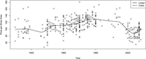
Historically the spline-fitting literature rejected linear splines on aesthetic grounds for being too jagged. But this was before shrinkage. Shrinkage can be done on cubic splines by penalizing the average second derivative of the spline curve (see Hastie, Tibshirani, and Friedman 2017), much like ridge regression penalizes the sum of squared parameters. The actuarial approach to linear spline shrinkage, following Barnett and Zehnwirth (2000), analogously shrinks the slope changes, which are the second differences of the splines. As Figure 1 shows, this does not differ much in jaggedness from the cubic spline fit. Another advantage is that the knots of the linear splines come out directly from the estimation as the points with zero slope change and so are determined simultaneously with the fits. This is a separate procedure with cubic splines, which makes the overall optimization more awkward.

Harezlak, Ruppert, and Wand (2018) recommended O’Sullivan penalized splines. These are a form of smoothing splines that meet a roughness penalty controlled by a smoothing constant $\lambda .$ They pick this $\lambda$ using “generalized cross-validation” from Craven and Wahba (1979). These splines are averages of a number of cubic functions and are not closed form, but there is software available to calculate them. They also discussed how to pick the number of knots $K$ for tying together the splines. They thought that with the smoothing done anyway, 35 knots spread out by the quantiles of the data would usually suffice. They did have some functions for testing the number of knots, however.

Actuarial smoothed linear splines can be done on any variables that can be ordered numerically 1, 2, 3, …. This is natural for years, ages, etc. but can make sense for class variables like vehicle use classes that have some degree of ranking involved. The parameter shrinkage is applied to the slope changes between two adjacent linear segments. Initially slope changes are allowed between all adjacent variables, but if the shrinkage reduces a slope change to zero, the line segment simply continues at that point, and a knot is eliminated.

Thus, the shrinkage chooses the knots, which can then determine how many are needed and put them where the curves most need to change. This is an advantage over the O’Sullivan splines, which usually use a fixed number like 35 knots spread according to the number of observations, not changes in the levels. In our experience, 35 knots is usually enough but can sometimes lead to overparameterization. The degree of shrinkage could be selected by loo cross-validation, which seems as good or better than generalized cross-validation once you have a posterior distribution available, but we use the fully Bayesian method of letting the conditional distribution of the degree of shrinkage given the data determine this. Bayesians tend to prefer this approach, as discussed at the end the subsection on goodness of fit from MCMC. The key to making this work is that you can create a design matrix with slope-change dummy variables, as discussed in Section 3.

A useful shortcut to the fitting when there are a lot of variables is to use lasso in an initial sorting out process. The R lasso program glmnet developed by Friedman, Hastie, and Tibshirani (2010) has a built-in cross-validation function cv.glmnet(), which we use with all of its standard defaults. It uses its own cross-validation method to select a range of $\lambda$ values that are worth considering. We take the low end of this range, which eliminates the fewest variables, as an initial selection point. Usually more variables are worth taking out, but this can happen later. Adjacent dummy variables are highly negatively correlated, and one can usually substitute for another with little change in the overall fit. This creates difficulties for MCMC, but lasso can quickly sort out the variables with the least overall contribution to the model and then MCMC can readily deal with those that remain. We did this in the Warsaw example and also in the mortality example in Section 4. Even if by chance a slope change is left out that would add value to the final model the impact is likely to be minimal.

An advantage of this method is that the fully Bayesian approach chooses the knots and the smoothing constant as parts of the posterior distributions and as noted above, fully Bayesian has less risk of producing a model with an exaggerated fit measure than cross-validation. Also being able to do this with just a design matrix and MCMC fitting software allows flexibility in model construction. More complex bilinear models like Lee-Carter, Renshaw-Haberman, and Hunt-Blake can be readily fit, as we shall see in Section 3. Further, it is straightforward to use any desired parameter distribution, like negative binomial in the example.

3. JOINT MORTALITY MODELING BY SHRINKAGE

We are using data from the Human Mortality Database (2019), which organizes tables by year of death and age at death. The year of birth is approximately year of death minus age at death, depending on whether the death is before or after the birthday in the year. For convenience, we consider cohort to be year of death minus age at death. Cohorts are denoted as n, with parameters $p[n],$ age at death by $u,$ with parameters $q[u],$ so the year of death is $w=n+u,$ with parameters $r[n+u].$ The data we use are, as is common, in complete age by year rectangles with a years and b ages and ab cells. These points are from $a+b-1$ cohorts, which have from 1 to min(a, b) ages in them. Any two of the indices n, u, w will identify a cell. We use n, u, which avoids subtraction of indices. Also, $c$ is a constant term which that is not shrunk in the modeling. The parameters add and multiply in the models to give the log of the mortality rate.

Initially the number of deaths is assumed Poisson in the mortality rate times the exposures, which are the number living at the beginning of the year. Theoretically, deaths counts are the sum of Bernoulli processes and so should be binomial, but for small probabilities the binomial is very close to the Poisson, which is sometimes easier to model. Later we test the Poisson assumption against heavier-tailed distributions.

3.1. Mortality Models

A basic model is the linear APC model. This has become fairly popular with actuaries and it is our starting point, because it is a purely linear model that can be estimated with standard packages, including lasso packages. Its log mortality rate $m[n,u]$ for cohort n and age u is given by $$m[n,u]=c+p\left[n\right]+q\left[u\right]+r[n+u].$$

With exposures e[n,u], the deaths $y[n,u]$ are often assumed to be Poisson distributed:

y[n, u] ∼Poisson (e[n, u]e^m[n,u]).

The model of Renshaw and Haberman (2006) adds cohorts to the Lee and Carter (1992) model, which itself allows the time trend $r[n+u]$ to vary by age, reflecting the fact that medical advances, etc. tend to improve the mortality rates for some ages more than others. Renshaw and Haberman (2006) also included trend weights on the cohort effects. We have tried that for other populations and found that the age effects were not consistent from one cohort to another. This aspect does not appear to have been widely used. Haberman and Renshaw (2011) did find that it improves the log-likelihood somewhat in one of three datasets they looked at. Chang and Sherris (2018) graphed the age effect for several cohorts of their data, which showed some variations among cohorts. They found that a two-parameter model for age variation within each cohort captured this well. We did not try this model. A more generalized underlying model with this same adjustment was discussed in Yajing, Sherris, and Ziveyi (2020).

Denoting the trend weight for age $u$ by $s[u],$ the Renshaw-Haberman model we use here is $$m[n,u]=c+p\left[n\right]+q\left[u\right]+s\left[u\right]r[n+u].$$

Hunt and Blake (2014) allowed the possibility of different trends with different age weights either simultaneously or in succession. This addresses a potential problem with the Lee-Carter model: The ages with the most mortality improvement can change over time. Venter and Şahin (2018) suggested an informal test for the need for multiple trends and found that they indeed helped in modeling the U.S. male population for ages 30–89. In the example here we fit the model to ages 50 and up and performed this test, which suggested that one trend is sufficient, so the model is presented in that form. It is then the same as the special case of the Renshaw-Haberman model with no age‒cohort interaction. In other populations we have noticed that modeling a wide range of ages over a long period can benefit from multiple trends.

The Renshaw-Haberman and Lee-Carter models are sometimes described as bilinear APC models, because they are linear if either the $s$ or $r$ parameters are taken as fixed constants. The age weights help model the real phenomenon of differential trends by age, but their biggest weakness is that they are fixed over the observation period, and the ages with the most trend can change over time as medical and public health trends change. The possibility of multiple trends in the Hunt-Blake model can reflect such changes.

3.2. Design Matrix

To set the basic APC model up to use linear modeling software packages, the entire array of death counts $y[n,u]$ is typically strung out into a single column $d[j]$ of length $ab.$ It is generally helpful to make parallel columns to record which age, period, and cohort cell $d[j]$ comes from. Then a design matrix can be created where all the variables $p[n],q[u],r[n+u]$ have columns parallel to the death counts, are represented as 0,1 dummy variables that have a 1 only for the observations that variable applies to. In practice we keep the constant $c$ out of the design matrix, and also leave out the first cohort, age, and year variables $p[1],q[1],r[1].$

Let $\beta$ be the vector of parameters and $\tilde{e}$ be the ab-vector of exposures corresponding to $d.$ Then the ab-vector $\widehat{m}$ of estimated log mortality rates is (1) $$\widehat{m}=c+X\beta$$(1) and (2) $$d\left[j\right]\sim \mathit{Poisson}\left(\tilde{e}\left[j\right]e^{\widehat{m}\left[j\right]}\right)$$(2)

Both formulas (1), (2) still hold when $X$ is singular, which can happen because of APC redundancy prior to shrinkage. In that case you cannot estimate $\beta$ as ${(X\prime X)}^{-1}X\prime d,$ but however it is estimated the fitted values are computed using (1), (2). These are the sampling statements that can be given to MCMC to create samples of the conditional distribution of the parameters given the data.

In the semiparametric case, where the parameters are slope changes to linear splines across the cohort, age, and year parameters, a different design matrix is needed. Slope changes are second differences in the piecewise-linear curves fit across each parameter type (age, period, etc.). The slope change variable for age i, for example, is zero at all points in d that are for ages less than i. It is 1 for all points for age i. The first differences have been increased by that parameter at that point as well. Therefore, any cell for age i + 1 gets the first difference plus the level value at age i, so it gets two summands of the age i variable. Thus, the dummy for that variable is 2 at those points. Then it is 3 at points for age i + 2, etc. In general, the age i dummy variable gets value ${(k-i+1)}_{+}$ at points for age k. The same formula works for the year i variable at points from year k, etc.

In the original levels design matrix, each row has three columns with a 1 in them. When a row is multiplied by $\beta ,$ those three values would pick out the year, age, and cohort parameters for that cell and they would be added up to get the $\widehat{m}$ value for the cell. In principle this is the same for the slope change design matrix but for any given row there would be nonzero elements for every year, age, and cohort up to that point. Those values would multiply the slope-change parameters in $\beta$ by the number of times that they add up for that cell and those would be summed to give $\widehat{m}.$

3.3. Fitting Procedure

For the two-population case, assume that the dependent variable $d$ column has all observations for the first population followed by all observations for the second population in the same order. Our approach is to fit a semiparametric model to the larger population and simultaneously fit a semiparametric model for the differences in the second population from the first. Then the smaller population parameters (in log form) are the sum of the two semiparametric models. With shrinkage applied, it is hoped that the difference parameters are smaller, so the second population would use fewer effective parameters than the first. The design matrix for the semiparametric fit to the second population differences is the same as the design matrix for either of the population’s log mortality rates. They all specify how many times each slope change parameter will be added up for each fitted value. The parameter vector will have parameters for the first population’s slope changes, followed by parameters for the slope change differences for the second population from the first. Because the constant term is not shrunk, it is not in the design matrix but is added in separately. The second population design matrix does include a constant variable for the difference, and that is shrunk. (In the symbolic equation below, the design matrix includes both constants.)

The Poisson mean vector is the element-by-element multiplication of the exposure vector with the exponentiation of the matrix multiplication of the design matrix by the parameter vector. This equation provides a visualization of the APC model with k parameters: $$E{\stackrel{\text{Death}\mathrm{ }\text{counts}(\tilde{d})}{\overbrace{\left(\begin{array}{c}\hfill \\ \text{First}\hfill \\ \text{Pop}.\hfill \\ \text{Counts}\hfill \\ \hfill \\ \hfill \\ \hfill \\ \hfill \\ \hfill \\ \text{Second}\hfill \\ \text{Pop}.\hfill \\ \text{Counts}\hfill \\ \hfill \end{array}\right)}}}_{2ab\times 1}={\stackrel{\text{Exposures}(\tilde{e})}{\overbrace{\left(\begin{array}{c}\hfill \\ \text{First}\hfill \\ \text{Pop}.\hfill \\ \text{Expo}-\hfill \\ \text{sures}\hfill \\ \hfill \\ \hfill \\ \hfill \\ \hfill \\ \text{Second}\hfill \\ \text{Pop}.\hfill \\ \text{Expo}-\hfill \\ \text{sures}\hfill \end{array}\right)}}}_{2ab\times 1}°\hspace{0.17em}\text{exp}\hspace{0.17em}{\stackrel{\text{Design}\mathrm{ }\text{matrix}}{\overbrace{\left(\begin{array}{cc}& \\ \text{All}\mathrm{ }\text{APC}\mathrm{ }\text{Variables}& \text{All}\mathrm{ }\text{Zeros}\mathrm{ }\text{for}\\ \text{Slope}\mathrm{ }\text{Change}& \text{First}\\ \text{Design}\mathrm{ }\text{Matrix}\mathrm{ }\text{for}& \text{Population}\\ \text{First}& \\ \text{Population}& \\ & \\ & \\ \text{Same}\mathrm{ }\text{Matrix}\mathrm{ }\text{to}\mathrm{ }\text{Give}& \text{Same}\mathrm{ }\text{Design}\mathrm{ }\text{Matrix}\\ \text{FirstPop}.& \text{But}\mathrm{ }\text{Now}\mathrm{ }\text{for}\\ \text{Model}\mathrm{ }\text{to}& \text{Difference}\mathrm{ }\text{Parameters}\\ \text{Second}& \text{for}\mathrm{ }\text{Slope}\mathrm{ }\text{Changes}\\ \text{Population}& \text{fortheSecondPop}.\end{array}\right)}}}_{2ab\times k}\times {\stackrel{\text{Parameter}\mathrm{ }\text{matrix}}{\overbrace{\left(\begin{array}{c}\hfill \\ \text{First}\hfill \\ \text{Pop}.\hfill \\ \text{Param}.\hfill \\ \hfill \\ \hfill \\ \text{Second}\hfill \\ \text{Pop}.\hfill \\ \text{Param}.\hfill \end{array}\right)}}}_{k\times 1}$$

The overall combined design matrix has four quadrants. All of the age, period, and cohort variables have columns for the first population and are repeated as columns for the second population’s difference variables. The first half of the rows is for the first population and the second half is for the second population. The upper left quadrant is just the single-population design matrix. The upper right quadrant is all zero, so the first population uses only its own variables. The lower left quadrant repeats the upper left quadrant, so the second population gets all of the parameter values from the first population. The same single-population design matrix is repeated in the lower right quadrant for the differences. Now this applies to the slope change variables for the second population differences. That population gets the sum of the parameters for the first population plus parameters of its own differences. If the difference parameters were not shrunk, the second population would end up with its own mortality parameters. If those parameters are all zero, the two populations would get the same parameters. The shrinkage lets the second population use the parameters from the first to the extent that they are relevant and then adds in changes as might be needed. Although the second population columns start off the same as the first, in the course of the fitting some variables with low t-statistics are forced to have parameters of zero by taking their columns out of the design matrix, and these variables could be different in the two populations.

MCMC is an effective way to search for good parameters, but these variables make it difficult. Consecutive variables are highly correlated; here, many are 99.9% correlated. There could be hundreds of variables in APC models for reasonably large datasets. It could take days or weeks to converge to good parameters running MCMC software on all of those correlated parameters. To speed this up, we start with lasso, which is usually very fast, to identify variables that can be eliminated and then use a reduced variable set for MCMC. Lasso software, like the R package glmnet, includes crossvalidation routines to help select $\lambda .$ This gives a range of $\lambda$ values that is worth considering. We use the lowest $\lambda$ value this suggests, which leaves the largest number of variables, to generate the starting variables for MCMC. Usually this still includes more parameters than are finally used in the model.

When a slope change variable is taken out, the slope of the fitted piecewise linear curve does not change at that point, which extends the previous line segment. If instead a small positive or negative value were to be estimated, the slope would change very slightly at that point, probably with not much change to the fitted values. When lasso cross-validation suggests that the slope change is not useful, would not add to the predictive value of the model. It is possible that a few of the omitted points in the end could have improved the model but they probably would not have made a lot of difference. So even with MCMC, there is no guarantee that all of the possible models have been examined and the very best selected. Nonetheless, this procedure is a reasonable way to get very good models.

Constraints are needed to get convergence of APC models. First of all, with the constant term included, the first age, period, and cohort parameters are set to zero. This is not enough to get a unique solution, however. With age, period, and cohort parameters all included, the design matrix is singular. The parameters are not uniquely determined in APC models in general: You can increase the period trend and offset that by decreasing the cohort trend, with adjustments as needed to the age parameters, and get exactly the same fitted values. Additional constraints can prevent this. A typical constraint is to force the cohort parameters to sum to 1.0. Venter and Şahin (2018) constrained the slope of the cohort parameters to be 0, which made the period trend the only trend so it can be interpreted as the trend given that there is no cohort trend. They also constrained the age weights on trend in Lee-Carter, etc. to be positive with the highest value $=1.$ This then makes the trend interpretable as the trend for the age with the highest trend. Another popular constraint is to instead make the trend weights sum to 1.0.

Some analysis of APC models takes the view that there are no true cohort and period trends because they only become specific after arbitrary constraints. But often there are things known or knowable about the drivers of these trends, like behavioral changes across generations, differences in medical technology, access to health care, etc., and these imply differences between time trend and cohort trend. Also, in Bayesian shrinkage and random effect models, two parameter sets with all of the same fitted values will not be equally likely. Their probabilities are proportional to the joint likelihood, which is the likelihood of the data times the postulated (or prior) distribution of the effects (or parameters). Because these are shrinkage distributions, a parameter closer to zero will have higher probability. Over a number of parameters, these will never be identical across the entire sample. Even though the design matrix is singular, there are still unique parameter sets with the highest probability.

It has been our experience that letting the parameters sort themselves out with no constraints usually gives a bit better fit, by loo, than you can get with the constraints. Parameter sets with lower prior probabilities show up less frequently in the posterior distribution, so the posterior mean gives a model with parameters closer to zero. Such a model would usually have a better fit by loo penalized likelihood though having the same log-likelihood as other fits. The loo penalty does not look at the size of parameters ― just at the out-of-sample predictions ― but these are better with properly shrunk parameters. You could say that fitting by shrinkage is itself a complicated type of constraint that does give unique parameters, but that these parameters do not have the ready interpretations that some constraints imply. Still, the better predictive accuracy measured by loo is some evidence, even if not totally definitive, that the trends estimated without other constraints better correspond to empirical reality. In this study we make the age weights on the period trend positive with a maximum of 1.0 but only constrain the trends themselves by Bayesian shrinkage.

Using slope change variables, with some eliminated, helps with identifiability. If a straight regression is done for a simple age‒period model, the slope change design matrix gives exactly the same $q,r$ parameter values that the 0,1 dummy matrix gives, and the APC matrix is still singular. But when enough slope changes are set to zero the matrix is no longer singular. Our procedure, then, is to use lasso for an AP design matrix, take out the slope change variables that lasso says are not needed, then add in all of the cohort variables, and run lasso again. The maximum variable set lasso finds for this is then the starting point for MCMC, without any other constraints on the variables.

The MCMC runs usually estimate a fair number of the remaining parameters as close to zero but with large standard deviations. This is analogous to having very low t statistics. We take out those variables as well but look at how loo changes. As long as loo does not get worse from this, those variables are left out. Usually a fair number of the variables that lasso identified are eliminated in this process. Leaving them in has little effect on the fit or the loo measure, but the data are more manageable without them. We use the best APC model produced by this as the starting point for the bilinear models, which add age modifiers to the period trends.

The steps we used to fit an APC model are as follows:

1. Make a slope change design matrix for the age and period variables and another one for the cohort variables.

2. Do a lasso run with the age and period variables only using cv.glmnet in default mode and list the coefficients for lambda.min. Take the variables with coefficients of zero out of the age‒period design matrix.

3. Add the cohort design matrix in with the remaining columns.

4. Run lasso again with cv.glmnet and list the coefficients for lambda.min. Take the variables with coefficients of zero out of the combined design matrix.

5. Run MCMC beginning with this design matrix and compute the loo fit measure. This is the end of the formal fitting procedure for the APC model, but next the low-t variables are taken out by the modeler as desired. The rule we used is like taking out the variables that reduce r-bar-squared in a standard regression, but is similarly problematic in using a fit measure to remove the variables. The following outlines how we did it, but other modelers may have their own approaches to this.

6. Look at the MCMC output and identify variables with high standard deviations and means near zero.

7. Take out these variables, run MCMC again, and compute loo.

8. If loo has improved, see whether there are more variables to take out, and repeat. If loo is worse, put some variables back in.

4. Swedish-Danish Male Mortality Example

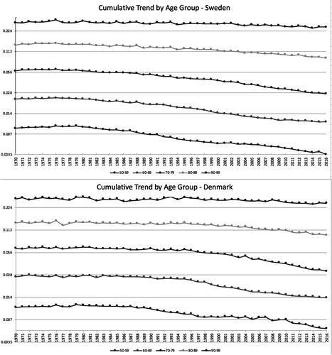
We model deaths from 1970 to 2016 for ages 50‒99 and cohorts 1883‒1953 from the Human Mortality Database (2019). Figure 2 graphs the cumulative mortality trends by age ranges for both populations to see whether there are any apparent shifts in the ages with the highest trend. The trends are a bit different in the two countries, but they look a lot like what the Lee-Carter model assumes, with the relative trends among the ages reasonably consistent over time.

FIGURE 2. Cumulative Trends by Age Group.

4.1. APC Model

Each population has 50 ages for 47 years coming from 71 cohorts. Leaving out the first age, period, and cohort of each population and adding the dummy variable for Denmark gives 331 variables for the APC design matrix. Table 1 has an excerpt from the design matrix, showing the first few age and cohort variables for Sweden for several observations.

TABLE 1 Excerpt of Design Matrix

Cohort	Year	Age	Deaths	r[2]	r[3]	r[4]	q[2]	q[3]	q[4]
1920	1970	50	305	0	0	0	37	36	35
1919	1970	51	306	1	0	0	36	35	34
1918	1970	52	344	2	1	0	35	34	33
1917	1970	53	359	3	2	1	34	33	32
1916	1970	54	384	4	3	2	33	32	31
1915	1970	55	417	5	4	3	32	31	30
1914	1970	56	496	6	5	4	31	30	29
1913	1970	57	570	7	6	5	30	29	28
1912	1970	58	569	8	7	6	29	28	27
1911	1970	59	605	9	8	7	28	27	26
1910	1970	60	732	10	9	8	27	26	25
1909	1970	61	781	11	10	9	26	25	24
1908	1970	62	793	12	11	10	25	24	23
1907	1970	63	854	13	12	11	24	23	22
1906	1970	64	953	14	13	12	23	22	21
1905	1970	65	943	15	14	13	22	21	20
1904	1970	66	1,003	16	15	14	21	20	19
1903	1970	67	1,092	17	16	15	20	19	18
1902	1970	68	1,156	18	17	16	19	18	17
1901	1970	69	1,192	19	18	17	18	17	16
1900	1970	70	1,266	20	19	18	17	16	15
1899	1970	71	1,237	21	20	19	16	15	14
1898	1970	72	1,324	22	21	20	15	14	13
1897	1970	73	1,338	23	22	21	14	13	12
1896	1970	74	1,414	24	23	22	13	12	11
1895	1970	75	1,317	25	24	23	12	11	10
1894	1970	76	1,481	26	25	24	11	10	9
1893	1970	77	1,363	27	26	25	10	9	8
1892	1970	78	1,323	28	27	26	9	8	7
1891	1970	79	1,311	29	28	27	8	7	6
1890	1970	80	1,294	30	29	28	7	6	5
1889	1970	81	1,262	31	30	29	6	5	4
1888	1970	82	1,187	32	31	30	5	4	3
1887	1970	83	1,189	33	32	31	4	3	2
1886	1970	84	1,075	34	33	32	3	2	1
1885	1970	85	1,024	35	34	33	2	1	0
1884	1970	86	842	36	35	34	1	0	0
1883	1970	87	764	37	36	35	0	0	0
1921	1971	50	334	0	0	0	38	37	36
1920	1971	51	352	1	0	0	37	36	35
1919	1971	52	330	2	1	0	36	35	34
1918	1971	53	363	3	2	1	35	34	33

We started with a lasso run, using the R GLM lasso package glmnet, without the cohort variables. The cv.glmnet app does the lasso estimation as well as this package’s default cross-validation. One of the outputs is the smallest $\lambda$ (thus the one with the most nonzero coefficients) that meets their cross-validation test. We ran the package twice. The first time was without the cohort variables and then with the resulting nonzero variables from the first run plus all of the cohort variables.

This resulted in 80 variables: 22 age variables, 16 year variables, and 42 cohort variables remained after lasso. We use the Stan MCMC application, specifically the R version, rstan, provided by Stan Development Team (2020). This requires specifying an assumed distribution for each parameter, and it simulates the conditional distribution of the parameters given the data. We used the double exponential distribution for all of the slope change variables. This is a fairly common choice, usually called Bayesian lasso, but we revisit it in Section 4.3. The double exponential distribution in Stan has a scale parameter $s=1/\lambda >0.$ An assumed distribution was provided for that, as well as for the constant term, as discussed below.

Eliminating the zero-coefficient variables enabled the APC model to be fit with no further constraints. Usually something like forcing the cohort parameters to have zero trend is needed for identifiability. That particular constraint means that the period trends can be interpreted as the trends given that they have all of the trend and none is in the cohorts. The method here is simpler and gives a bit better fit but does not allow for such an easy interpretation.

For positive parameters, we prefer to start with a distribution proportional to $1/x.$ This diverges both as $x$ gets small and as it gets large, so it gives balancing strong pulls up and down, whereas a positive uniform distribution diverges upwardly only, and this can bias the parameter upward. As an example where the integral is known, consider a distribution for the mean of a Poisson distribution with probability function proportional to $e^{-\beta }{\beta }^k.$ With a uniform distribution for $\beta ,$ which is proportional to 1, the conditional distribution of $\beta$ given an observation $k$ is also proportional to $e^{-\beta }{\beta }^k,$ which makes it a gamma in $k+1$ and 1, with mean $k+1.$ But if the distribution of $\beta$ is assumed proportional to $1/\beta ,$ the conditional is proportional to $e^{-\beta }{\beta }^{k-1},$ which makes it a gamma in $k,1,$ with mean $k.$ Thus, the $1/\beta$ unconditional distribution take the data at face value, whereas the uniform pushes it upwards. Numerical examples with other distributions find similar results.

The $1/\beta$ assumption is easier to implement in Stan by assuming log(β) is uniform. Stan just assumes that a uniform distribution is proportional to a constant, and so can be ignored. If not specified, it takes the range $\pm 1.7977·{10}^{308},$ which is the largest expressible in double-precision format. We usually start with a fairly wide range for uniform distributions, but if after working with the model for awhile the conditional distributions tend to end up in some narrower range, we tend to aim for something a bit wider than that range, mostly to save the program from searching among useless values. We ended up with assuming that the log of the constant is uniform on [‒8,‒3], with log(s) uniform on [‒6,‒3]. The parameter distributions ended up well within these ranges. Note that this happened to be set up as the constant for the log of the mortality and so is exponentiated twice in the final model but could have just as well have been set up as the log of the final constant.

The best purely APC model had 54 parameters, a loo measure of 22,158.5, and NLL of 22,081.7. The sample bias penalty, 76.8, is the difference between these. This penalty is a bit high for 54 parameters with shrinkage, which veteran Stan modelers tend to find suspicious in terms of predictive ability of the model. We know from the preliminary visual test that there is some variation in trend across the ages, and not reflecting this could be the problem.

4.2. Renshaw-Haberman Model

The next step was to put in the trend weights by age, which gives the Renshaw-Haberman model. This is no longer a simple linear model, which complicates the coding, though not substantially. We used the constraint that the highest weight for any age for a population would be 1.0, with all of the weights positive. In that way, the trend at any year is the trend for the age with the highest weight.

For this we needed a separate slope change design matrix $Y$ for trend weights, with 100 rows and columns, one for each age in each population. Y is to be multiplied by a column vector of 100 parameters that produce a vector of 50 trend weights for the first population and 50 for the second. For compactness, the variables with parameters close to zero were taken out, but this is not a necessary step and has minimal effect on the fitted values. When unneeded variables were eliminated, their columns were dropped but not the rows. Then the parameter vector $\eta$ times $Y$ gives the initial weights for each age. To make the weights positive with a maximum of 1.0, their maximum value is subtracted by population and then exponentiated to give the age weights $\alpha .$ $$\begin{array}{c}{\alpha }_1=Y\eta \\ \alpha =e^{{\alpha }_1-\mathit{max}({\alpha }_1)}\end{array}.$$

Now α has the trend weight for each age. These are multiplied by a 2ab × 100 0,1 design matrix with a 1 in each row, at the age and population column for that observation, giving A, a vector of the trend weights by observation. Next, the original design matrix columns are grouped into two parts: the design matrix $X$ and the parameter vector $\beta$ are only for the age and cohort parameters, and the original columns for the years go into design matrix $Z$ with parameters $\psi .$ $Z\psi$ then is the trend for the right year for each observation. This is multiplied pointwise by the vector A to give the weighted trend for each observation. Then (1) becomes (3) $$\widehat{m}=c+X\beta +A°(Z\psi ).$$(3)

This is not strictly a linear model because parameters α and ψ are combined multiplicatively. In the end, six more age, period, and cohort variables were eliminated, leaving 46 APC variables and 72 slope change variables, for 118 variables all together. This produced a loo penalized NLL of 20,725.5 and an NLL of 20,644.5, which are improvements of about 1,400 over the APC model. The penalty of 81.0 for the 118 variables is a more typical relationship for shrinkage models. NLL and penalized NLL are in logs, so it is the absolute difference, not the relative difference, that indicates how much improvement a better model produces. Here that is substantial, so Renshaw-Haberman is clearly better for these data.

4.3. Alternative Shrinkage Priors

Next we tried an alternative shrinkage distribution, as discussed in Section 3, using the variables from the best model. Instead of the double exponential priors, we assumed that the slope change variables were t distributed. A double exponential is roughly equivalent to a t with $\nu =6,$ a Cauchy is $\nu =1,$ and a normal is the limit as $\nu$ gets large. We tried a prior with log(v) uniform on [‒1,6]. That gives a range for $\nu$ of about [0.37 403]. The result was a slightly worse loo, at 20,726. The mean of $\nu$ was 2.4, with a median of 2. This is heavier tailed than the double exponential, with larger parameters allowed and smaller ones pushed more toward zero. Two more parameters came out <0.001 and can be eliminated.

We have found in other studies that loo does not change greatly with small changes in the heaviness of the shrinkage distribution tails, and it looked like estimating $\nu$ was using up degrees of freedom. Next we tried a constant $\nu =2$ and took out the two small trend weight variables. The result was then 116 variables, with a loo measure of 20,723.4, NLL of 20,643.9, and penalty of 79.5. Such a drop of 2 in the penalized NLL is usually considered a better model, and this one is more parsimonious as well.

4.4. Negative-Binomial Model

One assumption not checked so far is the Poisson distribution of deaths in each age‒period cell. As an alternative, we tried the negative binomial distribution, which has an additional parameter $\varphi ,$ which does not affect the mean but which makes the variance = ${\mu }^2/\varphi +\mu .$ This changes (2) to (4) $$d\left[j\right]\sim NB\left(\tilde{e}\left[j\right]e^{\widehat{m}\left[j\right]},\varphi \right).$$(4)

This actually gave a still lower NLL of 20,589.1 and loo of 20,648.1, and thus an improvement of 75. The sample bias penalty was much lower, at 59. There were also three fewer trend weight variables, leaving 67 of those, as well as 46 age, period, and cohort variables as before. Now there is still a constant, the shrinkage parameter, and $\varphi$ that are not shrunk, for 116 variables in total. The low penalty means that the log-likelihood of the omitted variables was not much worse than that of the full model, which is part of why the predictive measure loo was so much better.

The Poisson is an approximation to the binomial distribution that would come from a sum of independent Bernoulli processes. Having a more dispersed distribution suggests that there is some degree of correlation in the deaths. That could arise from high deaths in bad weather or disease outbreaks, for instance. However, the dispersion is a measure of the departure of the actual deaths from the fitted means and includes model error and estimation error. Thus, it is not entirely certain that the better fit implies that deaths are correlated.

We just assumed that log($\varphi$) was distributed uniform on $\pm 1.7977·{10}^{308}.$ The conditional mean of $\varphi$ given the data is 2,839. The largest mean for any cell was slightly above 2,000, and that would get a variance increased by 70%. This could be as little as a 10% increase for small cells. Compared to the Poisson, this makes it less critical to get a very close fit on the largest cells, which can give a better fit on the other cells. Of course, another reason for the better fit could be actual greater dispersion. The parameters graphed in Figures 3 to 6 are for the negative binomial model as are the actual verses. fitted values in Figures 7 and 8.

4.5. Fit Summaries

Table 2 summarizes the goodness-of-fit measures for all models. Table 3 shows the number of parameters of each type by country and the sum of their absolute values in the negative binomial model. As we were hoping, by doing the joint fitting, Denmark got fewer parameters and lower impact as measured by parameter absolute values. Thus, not so much change from the Sweden model was needed. Trend is a bit of an exception, and as we saw, Sweden does not have much trend whereas, Denmark has some. The mortality-by age parameters are one area in particular where the populations are similar, and Denmark does not need much change from the Sweden values. It is surprising how dominant the age weight parameters are in both size and count and also how they add so little to the NLL penalty and so much to the goodness of fit. They are clearly important in this model.

TABLE 2 Summary of Goodness-of-Fit Measures

	Parameters	Loo	Penalty	NLL
APC (Poisson with Laplace shrinkage)	54	22,159	77	22,082
Renshaw-Haberman (Poisson with Laplace shrinkage)	118	20,726	81	20,645
Renshaw-Haberman (Poisson with $\nu =2$ shrinkage)	116	20,723	79	20,644
Renshaw-Haberman (Negative. Binomial. with $\nu =2$ shrinkage)	116	20,648	59	20,589

TABLE 3 Parameter Count and Sum of Absolute Values for Negative Binomial Model

	Age	Cohort	Trend	Weight
Sweden count	10	15	5	34
Denmark count	3	9	4	33
Sweden sum |$\beta$|	0.126	0.062	0.054	0.363
Denmark sum |$\beta$|	0.022	0.041	0.093	0.189

Figure 3 shows the parametric curves fit to trend factors by population. Sweden has less trend in the later years. Denmark does not deviate from the Swedish trend until halfway through the period. Both show long stretches with few slope changes. These are a lot simpler than the empirical trend graph in Figure 1, which could be why the age weights are important. Figure 4 shows the curves for the age weights. They are more complex than the trends but still fairly smooth graphs. Denmark largely has the same overall pattern as Sweden and so is using its parameters to a fair degree. Figure 5 graphs the fitted age factors on a log scale, along with a rotation of the factors to horizontal, to better show their differences. There are some nuances of slope change variation that shows up in the rotation.

FIGURE 3. Trend Factors.

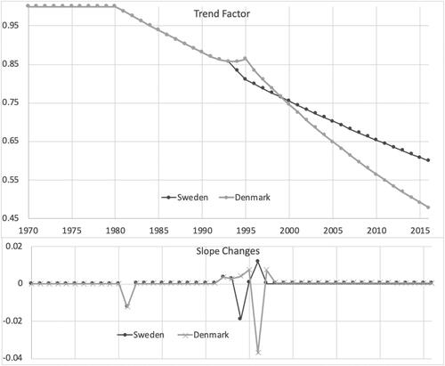
FIGURE 4. Trend Age Weights.

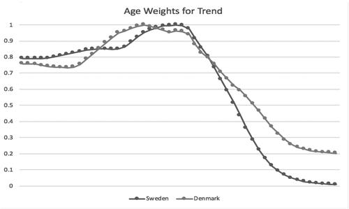
FIGURE 5. Age Factors.

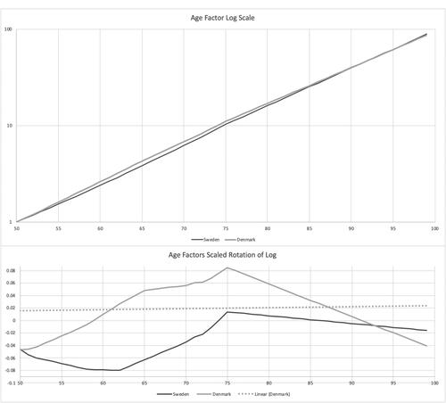
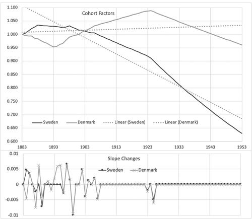
Figure 6 shows the cohort factors, along with fitted lines to each to show their average slopes. Although the shapes are different, a lot of the slope changes and differences from linear are actually similar between the two populations.

FIGURE 6. Cohort Factors.

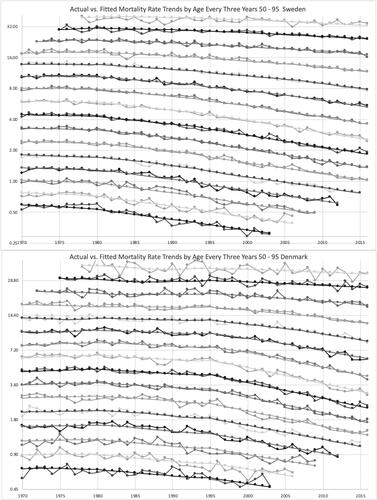
Actual versus. fitted mortality rates are graphed for the cohorts by age in 3-year ranges in Figure 7. The fitted values form smooth curves in this modeling. Denmark’s rates are more volatile, but the fitted values reasonably represent the trends in each country. For the most part, the rates are lower for later cohorts. The cohort parameters did not do exactly that, but the fitted rates are a combination of age, period, cohort, and trend weight parameters, which are all relative to each other. Figure 8 graphs this for year of death instead of cohort, and the conclusions are similar.

FIGURE 7. Actual vs. Fitted Age by Cohort.

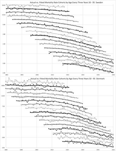
FIGURE 8. Actual vs. Fitted Age by Year.

In the example, the difference parameters for these second population are smaller and fewer than the parameters in the first model, suggesting that it is retaining features of the model of the larger population. For this data, the Renshaw-Haberman model fits better than the linear APC model, the negative binomial fits better than the Poisson, and using the t distribution with $\nu =2$ works well as an assumed shrinkage distribution. A more parsimonious model that looks not as good by loo can be obtained by a Cauchy shrinkage distribution (the t distribution with $\nu =1$), which could be a good idea if the model is regarded as an approximation to a more complex process. These shrinkage distributions also provide minimization formulas similar to those of lasso and ridge regression. The t with $\nu =2$ case, for instance, leads to minimization of NLL$+1.5\sum _{j}log(2+{\lambda }^2{\beta }_j^2).$

4.6. Projections

Projecting forward using these models would require projecting the period trends, and if more cohorts are to be included the cohort trends would need to be projected as well. With the fits that we have the period and cohort trends look remarkably stable for both countries. For over 20 years the period trend for Sweden has been constantly downward, at a factor of 0.991 per year. For Denmark the trend rate has been 0.987 over this period. These are the factors for ages 70–75, with less trend at other ages according to the curves fit to trend weight by age. A reasonable starting point would be to continue these trend rates. You could not expect declining mortality forever, but the rates are not very steep. After 50 years of decline at this rate, Sweden’s mortality at those ages would drop by a factor of 0.65 and Denmark’s by 0.51. Other ages would have less decline, and the deaths overall would shift to still older ages.

The cohort trends are less steep, with factors of 0.992 and 0.996 for Sweden and Denmark, respectively. Fifty years of compounding of these would give reduction factors of 0.69 for Sweden and 0.81 for Denmark. If these were to be combined, those born in 2003 would have lower mortality by 0.43 in Sweden and 0.41 in Denmark for the peak trend ages. Actuaries would naturally want to temper these trends with reasonable judgment if they were to use them in annuity and insurance pricing. In practice, pandemic issues would, of course, now go into their calculations. These countries have data through the Spanish flu pandemic that might influence their adjustments.

Stan can output the parameters for every sampled posterior point. The prior distributions can be used to simulate future outcomes for each sample, and these could be used for distributions around the projected mean results. These priors all have mean zero, which would be consistent with continuing the latest trends. The correlations across the parameters could also be computed over the historical period and applied during the simulations.

To use a model like this in practice, it would be important to review the parameter distributions. The Appendix has some R code for running these models. That includes code for printing and graphing the parameter distributions.

4.7. Population Behavioral Studies

Despite being among the countries with the longest life expectancy in the world from 1950 to 1980, Denmark experienced a dramatic fall in the rankings in the 1990s while Sweden maintained its position near the top. The difference in mortality between Denmark and Sweden has been discussed by several papers and Christensen et al. (2010) provided a comprehensive review and described the trends in overall mortality and cause-specific mortality with a discussion based on the underlying determinants of reduced life expectancy in Denmark. They showed that Denmark’s life expectancy improvement rates were close to zero between the late 1980s and early 1990s. Although in the mid-1990s, Denmark experienced an annual increase in life expectancy, Danish longevity has not been able to catch up with Sweden. Juel, Sorensen, and Bronnum-Hansen (2008) showed the significant impact of the risk factors such as alcohol consumption, smoking, physical inactivity, and unhealthy diet on Danish life expectancy. Christensen et al. (2010) emphasized the impact of smoking as the major explanation for the divergent Danish life expectancy trend compared to Sweden while acknowledging the contribution of different lifestyles and health care systems (investment in health care is lower in Denmark than in Sweden) in two countries. They also explained the reasons for the improvement in life expectancy in the early 1990s in Denmark as the effect of decreasing cardiovascular mortality, better lifestyles, better medical and surgical treatment, and better medical disease prevention services.

Looking at the fitted period trends in Figure 3 and the fitted cohort trends in Figure 6 shows that our model estimates the period trends as being pretty similar until the mid-1990s, with Denmark improving faster after that. However, the cohort trends are more favorable in Sweden. You could largely get the same overall effects by rotating the Swedish cohort curve up to match Denmark’s and rotate its period curve down. Either would correspond to the empirical relationship between the countries. But the actual results from the estimation are those that best match the conditional distribution of the parameters given the data that come with no constraints, as discussed at the end of Section 3. Both populations’ fits show sharp improvements beginning with cohorts born in the mid-1920s (who reached adulthood after WWII). This turn was slightly more in Denmark, but trends there had been upward before then, so Sweden maintained a faster rate of cohort improvement. Smoking was probably a key part of this. Denmark’s slowdown in mortality improvement in the 1990s corresponds to when their worst cohorts by our fits reached their 70s. The cohort fits suggest that the unhealthy behaviors found in the studies noted above were largely a cohort effect. That is something that the lifestyle measures may be able to test.

5. CONCLUSION

Joint APC modeling of related populations is a common need in actuarial work, including for mortality models and loss reserving. Semiparametric regression is a fairly new approach for actuaries and has advantages over MLE in producing lower estimation and prediction errors. We show how to apply it to individual mortality models by shrinking slope changes of linear spline fits to the parameters and then to modeling related datasets by shrinking changes in the semiparametric curves between the datasets.

MCMC estimation can be applied to complex modeling problems. We show how it can be used here to produce samples of the conditional distribution of the parameters given the data. This is typically done in a nominally Bayesian setting, where the model starts with postulated distributions of the parameters, called priors, and yields the conditional distribution of parameters given the data, called the posterior. But frequentist random effects modeling postulates distributions of the effects (which look like parameters to Bayesians) and there seems to be no reason why it could not also use MCMC to sample from the conditional distribution of the effects given the data. Furthermore, when Bayesians take this approach, they often feel free to depart from the traditional view of priors as incoming beliefs and treat them instead more like random effects; that is, postulated distributions. Thus, the approach we take appears largely consistent with Bayesian and frequentist approaches but differs slightly from the historical practices of each.

MCMC software can have problems with highly correlated variables like the slope change variables. Ridge regression and lasso were designed for this problem and can be much more efficient in estimating conditional modes. We use lasso, with only minor shrinkage, to eliminate the less necessary slope change variables and then use MCMC with the reduced parameter set. Common lasso software requires linear models, so we start off with a lasso Poisson regression for the linear APC model, with a log link, to reduce the variable set going into MCMC. We also present some advantages that MCMC shrinkage of linear spline slope changes has over the standard semiparametric use of O’Sullivan penalized splines.

Discussions on this article can be submitted until April 1, 2023. The authors reserve the right to reply to any discussion. Please see the Instructions for Authors found online at http://www.tandfonline.com/uaaj for submission instructions.

ACKNOWLEDGMENTS

The authors thank the anonymous reviewers for their comments and contributions.

APPENDIX. CODE EXAMPLES

First we look at performing a Poisson lasso run in R starting with a shrinkage design matrix. The cv.glmnet code exponentiates a regression model to give the Poisson means. If an offset is included, effectively the means before exponentiating are the offsets plus the regression fit, and have an offset for every observation. Thus, the offsets should be the logs of the exposures. The constant term is not in the design matrix but is added in.

library(readxl)library(glmnet)y = as.integer(scan(‘deaths.txt’)) # scan turns a column file into a vectorx = as.matrix(read_excel(“shrink_design_mat.xlsx”)) # spreadsheet has header rowoffs = scan(‘logexpo.txt’)fit = cv.glmnet(x, y, standardize = FALSE, family = “poisson”, offset = offs)out <- as.matrix(coef(fit, s = fit[dollar]lambda.min)) # these are the lasso parameterswrite.csv(out, file=”lasso_fit.csv”)This is possible Stan code mort_apc.stan for the APC case. The double exponential = Laplace prior is known as Bayesian lasso because the posterior mode is closely related to the lasso estimates.data { int N;//number of obs int U;//number of variables vector[N] expo; int y[N]; matrix[N,U] x;}parameters {//all except v will get uniform prior, which is defaultreal < lower=-8, upper=-3> cn;//constant term, starting in known rangereal < lower=-6, upper = -3> logs;//log of s, related to lambda, not too highvector[U] v;}transformed parameters {real s;   //shrinkage parametervector[N] mu;s = exp(logs);//makes 1/x prior for s > 0 to prevent biasmu = exp(cn + x*v);for (j in 1:N) mu[j] = mu[j]*expo[j];}model {//gives priors for those not assumed uniform. Choose this one for lasso.for (i in 1:U) v[i] double_exponential(0, s);//more weight to close to 0y poisson(mu);}generated quantities {//outputs log likelihood for loovector[N] log_lik;for (j in 1:N) log_lik[j] = poisson_lpmf(y[j] — mu[j]);}

This is R code for running the Stan code mort_apc.stan and conducting some analysis. The print command allows you to print out distribution ranges for each parameter with selected parameters and percentiles. Plot with show density plots all of the selected parameters as density graphs on a single scale. Plot with “hist” selected graphs histograms of each parameter’s posterior distribution. Extract gets all of the parameters by sample, but you have to be careful to check what order they come out in. One way to do this is just to keep the first chain, which here is mort_ss[,1,], and look at it as an array, which will have variable names as column headings. The order of the variables will be the same if you do it again with all of the chains. With the parameter sample distributions you can also compute the correlations among the parameters. These could be used along with the prior distributions to simulate parameter changes going forward to get projection ranges.

library(readxl) # allows reading excel files; assumes there is a header rowlibrary(“loo”)library(rstan)rstan_options(auto_write = TRUE)options(mc.cores = parallel::detectCores())# read in datax = as.matrix(read_excel(‘shrink_design_mat.xlsx’))y = as.integer(scan(‘deaths.txt’))expo = as.integer(scan(‘expo.txt’))N <- nrow(x)U <- ncol(x)c(N,U)df = list(N = N,U = U,expo = expo,y = y,x = x)# now run stanset.seed(8)mort_1 <- stan(file = ‘mort_apc.stan’, data = df, verbose = FALSE, chains = 4,iter = 2000, control = list(adapt_delta = 0.9, max_treedepth = 14))# compute loolog_spread_1 <- extract_log_lik(mort_1)loo_spread_1 <- loo(log_spread_1)loo_spread_1# output parameter means by chainout_mort_1 <- get_posterior_mean(mort_1)write.csv(out_mort_1, file=“out_apc.csv”)# show some outputplot(mort_1, pars = “v”, show_density = TRUE, ci_level = 0.8, fill_color = “black”)plot(mort_1, plotfun = “hist”, pars = “v”) #histograms for each parameterprint(mort_1, pars = c(“c”, “v”, “s”), probs = c(.025, 0.2, 0.5, 0.8, 0.975),digits_summary = 5)# get all samplesmort_ss = extract(mort_1, permuted = FALSE)# 3D array iterations by chains by parameters# can get rid of unneeded columns, concatenate to 2 dimensions, write out, etc.# array variables can be in different order than from get_posterior_mean# if you just keep 1 chain you can write out as .csv and it will have headings

REFERENCES

- Antonio, K., A. Bardoutsos, and W. Ouburg. 2015. Bayesian Poisson log-bilinear models for mortality projections with multiple populations. European Actuarial Journal 5:245–81. doi:10.1007/s13385-015-0115-6
- Barnett, G., and B. Zehnwirth. 2000. Best estimates for reserves. Proceedings of the Casualty Actuarial Society 87:245–303.
- Bühlmann, H. 1967. Experience rating and credibility. ASTIN Bulletin 4 (3):199–207. doi:10.1017/S0515036100008989
- Cairns, A. J. G., D. Blake, K. Dowd, G. D. Coughlan, and M. Khalaf-Allah. 2011. Bayesian stochastic mortality modelling for two populations. ASTIN Bulletin 41 (1):29–59.
- Chang, Y., and M. Sherris. 2018. Longevity risk management and the development of a value-based longevity index. Risks 6 (1):1–20.
- Christensen, K., M. Davidsen, K. Juel, L. Mortensen, R. Rau, and J. W. Vaupel. 2010. The divergent life-expectancy trends in Denmark and Sweden—And some potential explanations. In International differences in mortality at older ages: Dimensions and sources, ed. E. M. Crimmins, S. H. Preston, and B. Cohen, 385–408. Washington, DC: The National Academies Press. https://www.ncbi.nlm.nih.gov/books/NBK62592/pdf/Bookshelf_NBK62592.pdf.
- Craven, P., and G. Wahba. 1979. Smoothing noisy data with spline functions: Estimating the correct degree of smoothing by the method of generalized cross-validation. Numerische Mathematik 31:377–403. doi:10.1007/BF01404567
- Dowd, K., A. J. G. Cairns, D. Blake, G. D. Coughlan, D. Epstein, and M. Khalaf-Allah. 2011. A Gravity model of mortality rates for two related populations. North American Actuarial Journal 15 (2):334–56. doi:10.1080/10920277.2011.10597624
- Friedman, J., T. Hastie, and R. Tibshirani. 2010. Regularization paths for generalized linear models via coordinate descent. Journal of Statistical Software 33 (1):1–22. https://www.jstatsoft.org/article/view/v033i01. doi:10.18637/jss.v033.i01
- Gao, G., and S. Meng. 2018. Stochastic claims reserving via a Bayesian spline model with random loss ratio effects. ASTIN Bulletin 48 (1):55–88. doi:10.1017/asb.2017.19
- Gelfand, A. E. 1996. Model determination using sampling-based methods. In Markov Chain Monte Carlo in practice, ed. W. R. Gilks, S. Richardson, and D. J. Spiegelhalter, 145–62. London: Chapman and Hall.
- Haberman, S., and A. E. Renshaw. 2011. A comparative study of parametric mortality projection models. Insurance: Mathematics and Economics 48 (1):35–55. doi:10.1016/j.insmatheco.2010.09.003
- Harezlak, J., D. Ruppert, and M. P. Wand. 2018. Semiparametric regression with R. New York: Springer.
- Hastie, T., R. Tibshirani, and J. Friedman. 2017. The elements of statistical learning. Springer. https://web.stanford.edu/∼hastie/ElemStatLearn//printings/ESLII_print12.pdf.
- Hoerl, A. E., and R. Kennard. 1970. Ridge regression: Biased estimation for nonorthogonal problems. Technometrics 12:55–67. doi:10.1080/00401706.1970.10488634
- Human Mortality Database. 2019. University of California, Berkeley (USA), Max Planck Institute for Demographic Research (Germany) and United Nations. https://www.mortality.org/.
- Hunt, A., and D. Blake. 2014. A general procedure for constructing mortality models. North American Actuarial Journal 18 (1):116–38. doi:10.1080/10920277.2013.852963
- Jarner, S. F., and E. M. Kryger. 2009. Modelling adult mortality in small populations: The Saint model. Pensions Institute Discussion Paper PI-0902.
- Juel, K., J. Sorensen, and H. Bronnum-Hansen. 2008. Risk factors and public health in Denmark. Scandinavian Journal of Public Health 36 (Suppl. 1):112–227. . doi:10.1177/1403494800801101
- Lee, R., and L. Carter. 1992. Modeling and forecasting U.S. mortality. Journal of the American Statistical Association 87:659–75. doi:10.2307/2290201
- Li, N., and R. Lee. 2005. Coherent mortality forecasts for a group of populations: An extension of the Lee-Carter method. Demography 42 (3):575–94. doi:10.1353/dem.2005.0021
- Mowbray, A. H. 1914. How extensive a payroll exposure is necessary to give a dependable pure premium. Proceedings of the Casualty Actuarial Society 1:24–30.
- O’Sullivan, F. 1986. A statistical perspective on ill-posed inverse problems. Statistical Science 1 (4): 502–518.
- Renshaw, A. E., and S. Haberman. 2006. A cohort-based extension to the Lee-Carter model for mortality reduction factors. Insurance: Mathematics and Economics 38:556–70. doi:10.1016/j.insmatheco.2005.12.001
- Santosa, F., and W. W. Symes. 1986. Linear inversion of band-limited reflection seismograms. SIAM Journal on Scientific and Statistical Computing 7 (4):1307–30. doi:10.1137/0907087
- Stan Development Team. 2020. RStan: The R interface to Stan. http://mc-stan.org/.
- Stein, C. 1956. Inadmissibility of the usual estimator of the mean of a multivariate normal distribution. Proceedings of the Third Berkeley Symposium 1:197–206.
- Tibshirani, R. 1996. Regression shrinkage and selection via the lasso. Journal of the Royal Statistical Society. Series B (Methodological) 58 (1):267–88. doi:10.1111/j.2517-6161.1996.tb02080.x
- Tikhonov, A. N. 1943. On the stability of inverse problems. Doklady Akademii Nauk SSSR 39 (5):195–98.
- Vehtari, A., A. Gelman, and J. Gabry. 2017. Practical Bayesian model evaluation using leave-one-out cross-validation and WAIC. Journal of Statistics and Computing 27 (5):1413–32. doi:10.1007/s11222-016-9696-4
- Venter, G., R. Gutkovich, and Q. Gao. 2019. Parameter reduction in actuarial triangle models. Variance 12 (2):142–60.
- Venter, G., and S. Sahin. 2018. Parsimonious parameterization of age-period-cohort models by Bayesian shrinkage. ASTIN Bulletin 48 (1):89–110. doi:10.1017/asb.2017.21
- Yajing, X., M. Sherris, and J. Ziveyi. 2020. Continuous-time multi-cohort mortality modelling with affine processes. Scandinavian Actuarial Journal, 2020 (6):526–552. doi:10.1080/03461238.2019.1696223