Bivariate Mixed Poisson Regression Models with Varying Dispersion

Abstract

The main purpose of this article is to present a new class of bivariate mixed Poisson regression models with varying dispersion that offers sufficient flexibility for accommodating overdispersion and accounting for the positive correlation between the number of claims from third-party liability bodily injury and property damage. Maximum likelihood estimation for this family of models is achieved through an expectation-maximization algorithm that is shown to have a satisfactory performance when three members of this family, namely, the bivariate negative binomial, bivariate Poisson–inverse Gaussian, and bivariate Poisson–Lognormal distributions with regression specifications on every parameter are fitted on two-dimensional motor insurance data from a European motor insurer. The a posteriori, or bonus-malus, premium rates that are determined by these models are calculated via the expected value and variance principles and are compared to those based only on the a posteriori criteria. Finally, we present an extension of the proposed approach with varying dispersion by developing a bivariate Normal copula-based mixed Poisson regression model with varying dispersion and dependence parameters. This approach allows us to consider the influence of individual and coverage-specific risk factors on the mean, dispersion, and copula parameters when modeling different types of claims from different types of coverage. For expository purposes, the Normal copula paired with negative binomial distributions for marginals and regressors on the mean, dispersion, and copula parameters is fitted on a simulated dataset via maximum likelihood.

1. INTRODUCTION

The rapid advent of big data over the last few decades has motivated the need for constructing bivariate (and/or multivariate) regression models that can permit inferences about dependence structures that typically arise in high-dimensional count-valued data-sets based on explanatory variables. The main classes of models that have been widely applied in various fields of studies including, but not limited to, marketing, epidemiology, medical science, and finance are the bivariate (and/or multivariate) Poisson and mixed Poisson models and copula-based models. References, include, for example, Jung and Winkelmann (1993), Munkin and Trivedi (1999), Lee (1999), Gurmu and Elder (2000), Ho and Singer (2001), Kocherlakota and Kocherlakota (2001), Chib and Winkelmann (2001), Wang (2003), Alfò and Trovato (2004), Cameron et al. (2004), Karlis and Meligkotsidou (2005), Zimmer and Trivedi (2006), Park and Lord (2007), Winkelmann (2008), Ma, Kockelman, and Damien (2008), El-Basyouny and Sayed (2009), Aguero-Valverde and Jovanis (2009), Famoye (2010, 2012), Nikoloulopoulos and Karlis (2010), Ghitany et al. (2012), Cameron and Trivedi (2013), Nikoloulopoulos (2013a, 2013b), Zhan, Aziz, and Ukkusuri (2015), and Silva et al. (2017), among many others.

As far as ratemaking in non-life insurance, which is the main focus of this work, is concerned, the interested reader is referred to the articles by Bermúdez (2009), Bermúdez and Karlis (2011, 2012), and Shi and Valdez (2014b), who introduced different bivariate (and/or multivariate) regression and copula-based models and also pointed out the existence of a positive correlation between claim counts of two (and/or multiple) types of claims. Also, Bermúdez and Karlis (2017) were the first to take the Bayesian view for constructing two experience rating models, which integrate the a priori ratemaking based on bivariate Poisson regression models, extending the existing literature in the bivariate setting, which was confined on ratemaking models that were derived via the credibility approach. Additionally, it should be noted that recently many alternative approaches have been proposed in the literature for constructing flexible bivariate (and/or multivariate) insurance claim frequency regression models; see, for instance, Abdallah, Boucher, and Cossette (2016), Bermúdez, Guillén, and Karlis (2018), Pechon, Trufin, and Denuit (2018); Pechon, Denuit, and Trufin (2019, 2021), Bolancé and Vernic (2019), Denuit, Guillen, and Trufin (2019), Fung, Badescu, and Lin (2019a, 2019b), and Bolancé, Guillen, and Pitarque (2020).

In this study, we introduce a new class of bivariate mixed Poisson regression models with varying dispersion for modeling jointly bodily injury and property damage claim frequencies in motor third party liability (MTPL) insurance. This class is based on a mixing between two marginal Poisson distributions and a unit mean continuous prior, or mixing, distribution that belongs to a general distribution family including those that do not belong to the natural exponential family and/or are not conjugate to the Poisson. Within the adopted framework, both marginal mean parameters and the dispersion parameter are modeled jointly as parametric functions of explanatory variables.

In what follows, we provide a detailed discussion of our contributions, putting special emphasis on the suitability of the proposed family of models when dealing with MTPL claim count data in the bivariate setting, the maximum likelihood (ML) estimation procedure, and practical application aspects in the context of a posteriori ratemaking.

• Firstly, as is well known, the aim of compulsory MTPL insurance is to provide coverage against the bodily injuries and property damage that may inflicted on third parties during a motor vehicle–related accident. As empirical evidence has shown, bodily injury claims are less frequent than property damage claims but have the biggest impact on the insurance company’s claim expenditure. For example, according to a recent report by Insurance Europe (2019), even if in 2013 bodily injury claims only accounted for just under 14% of all MTPL claims recorded by European insurers, they represented 48.4% of all claims expenditure. Furthermore, on some occasions bodily injuries and property damage can be the result of the same accident because there are many factors in the MTPL insurance line that can simultaneously affect the joint dynamics of bodily injury and property damage claims. These are observable risk factors concerning the policyholders and their vehicles and differences among policyholders that cannot be observed by the actuary and give rise to positive correlation and overdispersion, which can be attributed to the excess of zeros and/or heavy upper tails (see Shared 1980) in MTPL bodily injury and property damage count data. It is natural to expect that the impact of such risks factors on the magnitude of the positive dependence between bodily injury and property damage claims could be different. For instance, this dependence might be stronger in urban regions and, in particular, in large cities than in small cities, and in the case of young drivers who are more likely to make more claims irrespective of the type. Also, as previous papers have concluded (see Bermúdez 2009; Bermúdez and Karlis 2017), even if the dependence between different claim types is not very strong, it must be taken into account in order to refine ratemaking. Additionally, in MTPL insurance the occurrence of bodily injury and property damage claims is strongly related to the unobserved heterogeneity, such as policyholders’ driving skills and habits and perception of the highway code, because both claim types are usually under the control of the driver. Therefore, in order to capture the influence of such factors to a good approximation, it is important to have all the necessary due diligence in place when constructing a bivariate claim frequency regression model for taking into account the relationship between MTPL bodily injury and property damage claims and a set of covariates when pricing the policies. Otherwise, a potential distribution misspecification can result in biased and unreliable parameter estimates, which, in turn may lead to inaccurate ratemaking that can result in nonnegligible financial implications for the company, because policyholders may switch to competing companies. The family of bivariate mixed Poisson regression models with varying dispersion we present in this article, can efficiently capture the complex features of two-dimensional MTPL data. In particular, our model class can accommodate overdispersion and account for positive dependencies between bivariate responses, which is what we expect from these data, in a very flexible manner because it permits for a variety of different distributional assumptions for the mixing density, which measures the level of unobservable risk associated with each policy and allows every parameter of the bivariate mixed Poisson model to be modeled in terms of important risk factors for both MTPL claim types, hence resulting in an improved risk evaluation. In order to emphasize the utility and generality of the proposed family of models, we focus on three of its members, namely, the bivariate negative binomial (BNB), bivariate Poisson–inverse Gaussian (BPIG), and bivariate Poisson–lognormal (BPLN) models with regression specifications on both their mean and dispersion parameters.

• Secondly, it is worth noting that the development of ML estimation procedures for joint modeling of all the parameters of mixed Poisson distributions in terms of covariate information remains a largely uncharted territory even within the univariate regression analysis context in the majority of both statistical and actuarial applications. In particular, regarding the statistical setting, this approach has only been explored so far by Rigby and Stasinopoulos (2005) and Barreto-Souza and Simas (2016). Rigby and Stasinopoulos (2005) proposed the generalized additive models for location, scale, and shape. The ML estimation of these regression-type models can be carried out using either the RS algorithm (see Rigby and Stasinopoulos 1996a, 1996b) or the CG algorithm (see Cole and Green 1992). Furthermore, Barreto-Souza and Simas (2016) used the expectation-maximization (EM) algorithm for fitting a general family of mixed Poisson regression models with varying dispersion. In their application they focused on the estimation of the negative binomial (NB) and Poisson–inverse Gaussian (PIG) regression models with regression structures on both their mean and dispersion parameters. Regarding the actuarial setting, Tzougas and Karlis (2020) implemented the EM algorithm for estimating the parameters of mixed exponential regression models with varying dispersion and Tzougas (2020) employed the EM algorithm for ML estimation in the Poisson–inverse Gamma (PIGA) regression model with varying dispersion. However, using the ML estimation procedure for the case when all parameters of bivariate mixed Poisson distributions are allowed to vary through covariates has not yet been addressed in the statistical or actuarial literature. The reason for this is because the log-likelihood of the mixed Poisson model becomes more complicated in the two-dimensional setting and hence allowing for regressors on every parameter further increases the computational burden, especially for members of the mixed Poisson family that have complicated densities that either are expressed in terms of special functions or cannot be written in a tractable closed form such as, for instance, the BPIG and BPLN models. The main achievement of this article is that it demonstrates that ML estimation for our class of bivariate mixed Poisson regression models with varying dispersion can be accomplished via an efficient and easily implementable EM-type algorithm that exploits the latent structure that is implied by the mixture representation of the bivariate mixed Poisson model and thus it reduces the problem of maximizing its joint likelihood function to the problem of maximizing the likelihood function of its mixing distribution.

• Thirdly, following the setup of Bermúdez and Karlis (2017), the proposed class of mixed Poisson regression models with varying dispersion will be used within the Bayesian paradigm for deriving a posteriori ratemaking mechanisms, or bonus-malus systems. At this point we would like to call attention to the fact that, because the posterior claim frequency distribution is expressed in terms of both mean parameters and the dispersion parameter of the bivariate mixed Poisson model, using regressors on every parameter results in better risk-adjusted a posteriori, or bonus-malus, premiums. More important, because the motor insurance market is highly competitive, our family of models is well justified for use in practice, because it can enable the actuary to set fair and equitable premiums based on a sound risk measuring basis. These premiums tailor-made to the risk involved are calculated based on the expected value and variance principles,¹ providing the company with useful alternative tariff structures.

Finally, it is important to note that when modelling different types of claims from different types of coverage, such as, for example, motor and home insurance bundled into a single policy, the mean, dispersion, and dependence components of a bivariate claim count model may be influenced by different individual and coverage-type risk characteristics. However, in the case of the bivariate mixed Poisson regression model with varying dispersion, the dispersion parameter can only be modeled using common covariates for both claim types. Moreover, in such cases, the dependence between the different claim count response variables may not necessarily be positive. Therefore, it is interesting to extend the proposed modeling framework by pairing a bivariate Normal copula with a dependence parameter that can vary through covariates with mixed Poisson regression models with varying dispersion. Under this general approach, in addition to the mean parameters, the dispersion and copula parameters of the model can vary through covariate information regarding different coverage types and the policyholders. For demonstration purposes, the bivariate Normal copula-based NB regression model with varying dispersion and dependence parameters is fitted on a simulated data set using ML estimation.

The remainder of this article proceeds as follows. In Section 2 we provide an in depth description of the proposed class of bivariate mixed Poisson regression models with varying dispersion. Also, we derive the joint probability mass function (jpmf) of the BNB, BPIG, and BPLN regression models with varying dispersion. Section 3 describes the ML estimation via the EM algorithm. Furthermore, we consider detailed EM algorithms for the BNB, BPIG, and BPLN regression models with varying dispersion. In Section 4 we calculate the a posteriori premiums using the expected value and variance principles. Section 5 presents the derivation of the bivariate Normal copula-based mixed Poisson regression model with varying dispersion and dependence parameters. In Section 6 the BNB, BPIG, and BPLN models are fitted on a real MTPL dataset. Also, the a posteriori premiums determined by these models are computed. Additionally, the bivariate Normal copula-based NB regression model with varying dispersion and dependence parameters is fitted on a simulated data set. Finally, concluding remarks are given in Section 7.

2. THE BIVARIATE MIXED POISSON REGRESSION MODEL WITH VARYING DISPERSION

The general class of bivariate mixed Poisson regression models with varying dispersion that we consider in this article can be described as follows.

Assume that the individual claim frequencies $K_{i,j},$ where i = 1 denotes the MTPL bodily injury claims and i = 2 denotes the MTPL property damage claims, arising from a policyholder j, $j=1,\dots ,n,$ are independent per j and consider that given the random variables Z_j > 0, $K_{i,j}|Z_j$ per claim type i = 1, 2, are distributed according to a Poisson distribution with probability mass function (pmf) given by (1) $$f\left(k_{i,j}|z_j\right)=\frac{\hspace{0.17em}\text{exp}[-({\mu }_{i,j}{z}_j)]{({\mu }_{i,j}{z}_j)}^{k_{i,j}}}{k_{i,j}!},$$(1) for $k_{i,j}=0,1,2,3,\dots ,$ where ${\mu }_{i,j}>0,$ with mean and variance $\mathbb{E}(k_{i,j}|z_j)={\mu }_{i,j}{z}_j$ and $\text{Var}(k_{i,j}|z_j)={\mu }_{i,j}{z}_j.$

Furthermore, suppose that Z_j are random variables from a continuous and at least twice-differentiable mixing distribution with probability density function (pdf) $g(z_j;{\sigma }_j),$ where we assume that $\mathbb{E}(Z_j)=1$ because this ensures that the model is identifiable and where ${\sigma }_j>0$ is the dispersion parameter.

Therefore, considering the previous assumptions, we can easily see that the unconditional distribution of $K_{i,j}$ is a bivariate mixed Poisson distribution with joint probability mass function (jpmf) given by (2) $$f\left(k_{1,j},k_{2,j}\right)=\underset{0}{\overset{\infty }{\int }}\prod _{i=1}^{2}f\left(k_{i,j}|z_j\right)g\left(z_j;{\sigma }_j\right)d{z}_j.$$(2)

To allow the two mean parameters and the dispersion parameter to be modeled in terms of explanatory variables with parametric linear functional forms we consider that (3) $${\mu }_{1,j}=\hspace{0.17em}\text{exp}\hspace{0.17em}({\mathit{x}}_{\mathit{1},\mathit{j}}{}^T{\mathit{\beta }}_{\mathit{1}})$$(3) (4) $${\mu }_{2,j}=\hspace{0.17em}\text{exp}\hspace{0.17em}({\mathit{x}}_{\mathit{2},\mathit{j}}{}^T{\mathit{\beta }}_{\mathit{2}})$$(4) (5) $${\sigma }_j=\hspace{0.17em}\text{exp}\hspace{0.17em}({\mathit{x}}_{\mathit{3},\mathit{j}}{}^T{\mathit{\beta }}_{\mathit{3}}),$$(5) where ${\mathit{x}}_{\mathit{1},\mathit{j}},{\mathit{x}}_{\mathit{2},\mathit{j}},$ and ${\mathit{x}}_{\mathit{3},\mathit{j}}$ are vectors of covariates with dimensions $p_1\times 1,p_2\times 1,$ and $p_3\times 1,$ respectively, with ${({\beta }_{1,1},\dots ,{\beta }_{1,p_1})}^T,{({\beta }_{2,1},\dots ,{\beta }_{2,p_2})}^T,$ and ${({\beta }_{3,1},\dots ,{\beta }_{3,p_3})}^T$ the corresponding parameter vectors and where it is assumed that the matrices ${\mathbf{X}}_{\mathbf{1}},{\mathbf{X}}_{\mathbf{2}},$ and ${\mathbf{X}}_{\mathbf{3}},$ with rows given by $x_{1,i},x_{2,i},$ and $x_{3,i}$ respectively, are of full rank.

Finally, the following properties associated with the proposed bivariate mixed Poisson regression model with varying dispersion ensure its flexibility in the context of MTPL insurance:

1. The marginal distribution of $K_{i,j},$ for i = 1, 2, is the same mixed Poisson distribution as its bivariate counterpart. Also, the mean and the variance of $K_{i,j}$ are (6) $$\mathbb{E}\left(K_{i,j}\right)={\mu }_{i,j}$$(6) and (7) $$\text{Var}\left(K_{i,j}\right)={\mu }_{i,j}\left[1+{\mu }_{i,j}\text{Var}(Z_j)\right].$$(7)

2. The covariance (Cov) between $K_{1,j}$ and $K_{2,j}$ is given by (8) $$\text{Cov}\left(K_{1,j},K_{2,j}\right)={\mu }_{1,j}{\mu }_{2,j}\text{Var}(Z_j)\hspace{1em}i=1\ne i=2.$$(8)

3. The correlation (Corr) between $K_{1,j}$ and $K_{2,j}$ is given by (9) $$\text{Corr}\left(K_{1,j},K_{2,j}\right)=\frac{\text{Var}(Z_j)\sqrt{{\mu }_{1,j}{\mu }_{2,j}}}{\sqrt{(1+{\mu }_{1,j}\text{Var}(Z_j))(1+{\mu }_{2,j}\text{Var}(Z_j))}}.$$(9)

4. The generalized variance ratio (GVR) between a bivariate mixed Poisson model with varying dispersion––that is, $K_{i,j}\sim \text{Poisson}({\mu }_{i,j}{z}_j)$––with $Z_j\sim g(z_j;{\sigma }_j),$ which is the pdf of the mixing density, and a simple Poisson model––that is, $Y_{i,j}\sim \text{Poisson}({\mu }_{i,j})$––is given by (10) $$\text{GVR}=\frac{\sum _{i=1}^2\text{Var}\left(K_{i,j}\right)+2\sum _{i<l}\text{Cov}\left(K_{i,j},K_{l,j}\right)}{\sum _{i=1}^2\text{Var}\left(Y_{i,j}\right)}=1+\text{Var}(Z_j)\sum _{i=1}^2{\mu }_{i,j}.$$(10)

As it can be seen from Equations (9)(9) $$\text{Corr}\left(K_{1,j},K_{2,j}\right)=\frac{\text{Var}(Z_j)\sqrt{{\mu }_{1,j}{\mu }_{2,j}}}{\sqrt{(1+{\mu }_{1,j}\text{Var}(Z_j))(1+{\mu }_{2,j}\text{Var}(Z_j))}}.$$(9) and (10)(10) $$\text{GVR}=\frac{\sum _{i=1}^2\text{Var}\left(K_{i,j}\right)+2\sum _{i<l}\text{Cov}\left(K_{i,j},K_{l,j}\right)}{\sum _{i=1}^2\text{Var}\left(Y_{i,j}\right)}=1+\text{Var}(Z_j)\sum _{i=1}^2{\mu }_{i,j}.$$(10) , $\text{Corr}(K_{1,j},K_{2,j})>0$ and GVR > 1. Also, the GVR increases as the variance of the mixing distribution increases. Thus, as was previously mentioned, the bivariate mixed Poisson regression model allows for the positive correlation between the MTPL bodily injury and property damage claims and accommodates overdispersion.

In what follows, different bivariate mixed Poisson distributions with regression structures on every parameter are used to describe the behavior of the number of bodily injury and property damage claims as a function of the explanatory variables including the BNB, BPIG, and BPLN distributions.

2.1. BNB Regression Model with Varying Dispersion

Let Z_j follow a Gamma distribution with a pdf (11) $$g(z_j;{\sigma }_j)=\frac{\hspace{0.17em}\text{exp}[-{\sigma }_j{z}_j]{\sigma }_j^{{\sigma }_j}}{\Gamma ({\sigma }_j)}{z}_j^{{\sigma }_j-1},$$(11) where ${\sigma }_j>0,$ with mean and variance (12) $$\mathbb{E}(Z_j)=1$$(12) and (13) $$\text{Var}(Z_j)=1/{\sigma }_j,$$(13) for $j=1,\dots ,n.$

Thus, based on Equations (1)(1) $$f\left(k_{i,j}|z_j\right)=\frac{\hspace{0.17em}\text{exp}[-({\mu }_{i,j}{z}_j)]{({\mu }_{i,j}{z}_j)}^{k_{i,j}}}{k_{i,j}!},$$(1) and (11)(11) $$g(z_j;{\sigma }_j)=\frac{\hspace{0.17em}\text{exp}[-{\sigma }_j{z}_j]{\sigma }_j^{{\sigma }_j}}{\Gamma ({\sigma }_j)}{z}_j^{{\sigma }_j-1},$$(11) it is easy to see that the resulting distribution is the BNB distribution with jpmf (14) $$f(k_{1,j},k_{2,j})=\frac{\Gamma ({\sigma }_j+\sum _{i=1}^2{k}_{i,j})}{\Gamma ({\sigma }_j)\prod _{i=1}^2{k}_{i,j}!}\frac{{\sigma }_j^{{\sigma }_j}\prod _{i=1}^2{({\mu }_{i,j})}^{k_{i,j}}}{{({\sigma }_j+{\mu }_{i,j})}^{{\sigma }_j+\sum _{i=1}^2{k}_{i,j}}}.$$(14)

2.2. BPIG Regression Model with Varying Dispersion

Let Z_j follow an Inverse Gaussian distribution with a pdf of the form (15) $$g(z_j;{\sigma }_j)=\frac{{\sigma }_j}{\sqrt{2\pi }}{z}_j^{-3/2}\hspace{0.17em}\text{exp}[{\sigma }_j^2-\frac{{\sigma }_j^2}{2}(\frac{1}{z_j}+z_j\left)\right],$$(15) where ${\sigma }_j>0,$ with mean and variance (16) $$\mathbb{E}(Z_j)=1$$(16) and (17) $$\text{Var}(Z_j)=1/{\sigma }_j^2,$$(17) for $j=1,\dots ,n.$

Therefore, considering the assumptions in Equations (1)(1) $$f\left(k_{i,j}|z_j\right)=\frac{\hspace{0.17em}\text{exp}[-({\mu }_{i,j}{z}_j)]{({\mu }_{i,j}{z}_j)}^{k_{i,j}}}{k_{i,j}!},$$(1) and (15)(15) $$g(z_j;{\sigma }_j)=\frac{{\sigma }_j}{\sqrt{2\pi }}{z}_j^{-3/2}\hspace{0.17em}\text{exp}[{\sigma }_j^2-\frac{{\sigma }_j^2}{2}(\frac{1}{z_j}+z_j\left)\right],$$(15) it can be verified that the resulting distribution is the BPIG distribution with jpmf (18) $$f(k_{1,j},k_{2,j})=\frac{2{\sigma }_j\hspace{0.17em}\text{exp}\hspace{0.17em}({\sigma }_j^2)}{\sqrt{2\pi }}{K}_{{\sum }_{i=1}^2{k}_{i,j}-\frac{1}{2}}({\sigma }_j{\Delta }_j){(\frac{{\sigma }_j}{{\Delta }_j})}^{{\sum }_{i=1}^2{k}_{i,j}-\frac{1}{2}}\prod _{i=1}^2\frac{{\mu }_{i,j}^{k_{i,j}}}{k_{i,j}!},$$(18) where ${\Delta }_j=\sqrt{{\sigma }_j^2+2{\sum }_{i=1}^2{\mu }_{i,j}}$ and $K_{\nu }(\omega )$ denotes the modified Bessel function of the third kind of order ν and argument ω.

2.3. BPLN Regression Model with Varying Dispersion

Let Z_j follow an Lognormal distribution with a pdf of the form (19) $$g(z_j;{\sigma }_j)=\frac{\hspace{0.17em}\text{exp}[-\frac{{(\hspace{0.17em}\text{log}\hspace{0.17em}(z_j)+{\sigma }_j^2/2)}^2}{2{\sigma }_j^2}]}{\sqrt{2\pi }{\sigma }_j{z}_j},$$(19) where ${\sigma }_j>0,$ with mean and variance (20) $$\mathbb{E}(Z_j)=1$$(20) and (21) $$\text{Var}(Z_j)=\hspace{0.17em}\text{exp}\hspace{0.17em}({\sigma }_j^2)-1,$$(21) for $j=1,\dots ,n.$

Thus, based on Equations (1)(1) $$f\left(k_{i,j}|z_j\right)=\frac{\hspace{0.17em}\text{exp}[-({\mu }_{i,j}{z}_j)]{({\mu }_{i,j}{z}_j)}^{k_{i,j}}}{k_{i,j}!},$$(1) and (19)(19) $$g(z_j;{\sigma }_j)=\frac{\hspace{0.17em}\text{exp}[-\frac{{(\hspace{0.17em}\text{log}\hspace{0.17em}(z_j)+{\sigma }_j^2/2)}^2}{2{\sigma }_j^2}]}{\sqrt{2\pi }{\sigma }_j{z}_j},$$(19) it is easy to see that the resulting distribution is the BPLN distribution with jpmf (22) $$f(k_{1,j},k_{2,j})={\int }_0^{\infty }\prod _{i=1}^2\frac{\hspace{0.17em}\text{exp}[-({\mu }_{i,j}{z}_j)]{({\mu }_{i,j}{z}_j)}^{k_{i,j}}}{k_{i,j}!}\frac{\hspace{0.17em}\text{exp}[-\frac{{(\hspace{0.17em}\text{log}\hspace{0.17em}(z_j)+{\sigma }_j^2/2)}^2}{2{\sigma }_j^2}]}{\sqrt{2\pi }{\sigma }_j{z}_j}d{z}_j,$$(22) which could not be written in closed form and hence numerical integration is required.

3. THE EM ALGORITHM

In this section we describe how the EM algorithm (see Dempster, Laird, and Rubin 1977; McLachlan and Krishnan 2007) can be employed for facilitating ML estimation of the parameters of the bivariate mixed Poisson regression model for marginal means and dispersion described in Section 2.

Let $(k_{1,j},k_{2,j},{\mathit{x}}_{\mathit{1},\mathit{j}},{\mathit{x}}_{\mathit{2},\mathit{j}},{\mathit{x}}_{\mathit{3},\mathit{j}}),$ $j=1,\dots ,n,$ be a sample of independent observations, where $K_{1,j}$ and $K_{2,j}$ are the response variables and ${\mathit{x}}_{\mathit{1},\mathit{j}},{\mathit{x}}_{\mathit{2},\mathit{j}},$ and ${\mathit{x}}_{\mathit{3},\mathit{j}}$ are the vectors of covariate information with dimensions $p_1\times 1,$ $p_2\times 1,$ and $p_3\times 1,$ respectively. Also, suppose that the data are produced according to the bivariate mixed Poisson model. Then, the log-likelihood of the model can be written as (23) $$l\left(\mathit{\theta }\right)=\sum _{i=1}^n\hspace{0.17em}\text{log}\hspace{0.17em}\left(f\left(k_{1,j},k_{2,j}\right)\right),$$(23) where $\mathit{\theta }={({\mathit{\beta }}_{\mathit{1}}{}^T,{\mathit{\beta }}_{\mathit{2}}{}^T,{\mathit{\beta }}_{\mathit{3}}{}^T)}^T$ is the vector of the parameters and where $f(k_{1,j},k_{2,j})$ is the jpmf of the bivariate mixed Poisson model, which is given by Equation (2)(2) $$f\left(k_{1,j},k_{2,j}\right)=\underset{0}{\overset{\infty }{\int }}\prod _{i=1}^{2}f\left(k_{i,j}|z_j\right)g\left(z_j;{\sigma }_j\right)d{z}_j.$$(2) .

Direct maximization of Equation (23)(23) $$l\left(\mathit{\theta }\right)=\sum _{i=1}^n\hspace{0.17em}\text{log}\hspace{0.17em}\left(f\left(k_{1,j},k_{2,j}\right)\right),$$(23) with respect to the vector of parameters $\mathit{\theta }$ is cumbersome because the log-likelihood of the bivariate mixed Poisson model is not usually tractable. Moreover, when both mean parameters and the dispersion parameter are modeled as functions of explanatory variables, this raises additional computational challenges.

Fortunately, ML estimation can be accomplished relatively easily via an EM-type algorithm that is specifically tailored to ML estimation for univariate and bivariate (and/or multivariate) mixed Poisson models (see, for instance, Karlis 2001, 2005; Ghitany et al. 2012; Barreto-Souza and Simas 2016; Tzougas 2020) because their stochastic mixture representation involving a nonobservable random variable, denoted by Z_j herein, can be considered to produce missing data. In our case, by augmentation of the unobserved Z_j one can write the complete log-likelihood as follows: (24) $$l_c\left(\mathbf{\theta }\right)=\sum _{i=1}^2\sum _{j=1}^n\left[-{\mu }_{i,j}{z}_j+k_{i,j}\hspace{0.17em}\text{log}\hspace{0.17em}\left({\mu }_{i,j}{z}_j\right)-\hspace{0.17em}\text{log}\hspace{0.17em}\left(k_{i,j}!\right)\right]+\sum _{j=1}^n\hspace{0.17em}\text{log}\hspace{0.17em}\left(g\left(z_j;{\sigma }_j\right)\right),$$(24) for i = 1, 2 and $j=1,\dots ,n,$ where $g(z_j;{\sigma }_j)$ is the pdf of the mixing distribution and where ${\mu }_{i,j}$ and σ_j are given by Equations (3)(3) $${\mu }_{1,j}=\hspace{0.17em}\text{exp}\hspace{0.17em}({\mathit{x}}_{\mathit{1},\mathit{j}}{}^T{\mathit{\beta }}_{\mathit{1}})$$(3) , (4)(4) $${\mu }_{2,j}=\hspace{0.17em}\text{exp}\hspace{0.17em}({\mathit{x}}_{\mathit{2},\mathit{j}}{}^T{\mathit{\beta }}_{\mathit{2}})$$(4) and (5)(5) $${\sigma }_j=\hspace{0.17em}\text{exp}\hspace{0.17em}({\mathit{x}}_{\mathit{3},\mathit{j}}{}^T{\mathit{\beta }}_{\mathit{3}}),$$(5) , respectively.

The E- and the M-steps of our EM-type algorithm procedure for the bivariate mixed Poisson regression model with varying dispersion are described below, including a few comments for each step.

• E-Step:

  The $Q$-function, which is the conditional expectation of the complete data log-likelihood in Equation (24)(24) $$l_c\left(\mathbf{\theta }\right)=\sum _{i=1}^2\sum _{j=1}^n\left[-{\mu }_{i,j}{z}_j+k_{i,j}\hspace{0.17em}\text{log}\hspace{0.17em}\left({\mu }_{i,j}{z}_j\right)-\hspace{0.17em}\text{log}\hspace{0.17em}\left(k_{i,j}!\right)\right]+\sum _{j=1}^n\hspace{0.17em}\text{log}\hspace{0.17em}\left(g\left(z_j;{\sigma }_j\right)\right),$$(24) , is calculated in a general way to elucidate its features for our general class of bivariate mixed Poisson regression models with varying dispersion (25) $$\begin{array}{c}Q\left(\mathit{\theta };{\mathit{\theta }}^{\left(r\right)}\right)\equiv {\mathbb{E}}_{z_j}\left(l_c\left(\mathit{\theta }\right)|k_{1,j},k_{2,j};{\mathit{\theta }}^{\left(r\right)}\right)\propto \\ \propto \sum _{i=1}^2\sum _{j=1}^n\left[-{\mu }_{i,j}{\mathbb{E}}_{z_j}\left[z_j|k_{i,j};{\mathbf{\theta }}^{\left(r\right)}\right]+k_{i,j}\hspace{0.17em}\text{log}\hspace{0.17em}\left({\mu }_{i,j}\right)\right]\\ +\sum _{j=1}^n{\mathbb{E}}_{z_j}\left[\text{log}\hspace{0.17em}\left(g\left(z_j;{\sigma }_j^{\left(r\right)}\right)\right)\right],\end{array}$$(25) where ${\mathit{\theta }}^{(r)}$ is the estimate of $\mathit{\theta }$ at the rth iteration in the E-step of our EM algorithm. Then, compute the pseudo-values $w_j={\mathbb{E}}_{z_j}\left[z_j|k_{i,j};{\mathit{\theta }}^{(r)}\right]$ and ${\lambda }_{k,j}={\mathbb{E}}_{z_j}\left[s_k(z_j)|k_{i,j};{\mathit{\theta }}^{(r)}\right],$ for i = 1, 2, $j=1,..,n$ and $k=1,\dots .,\nu ,$ where $s_k(.)$ are certain functions² that are involved in the terms needed for maximizing the part of the $Q$-function that corresponds to the conditional expectation of the log-likelihood of $g(z_j;{\sigma }_j).$

• M-Step:

  Using the pseudo-values w_j and ${\omega }_{k,j}$ from the E-step and the Newton-Raphson algorithm three times,³ find the maximum global point ${\mathit{\theta }}^{(r+1)}$ of the $Q$-function; that is, obtain the updated estimates ${\mathit{\beta }}_{\mathit{1}}{}^{(r+1)},{\mathit{\beta }}_{\mathit{2}}{}^{(r+1)},$ and ${\mathit{\beta }}_{\mathit{3}}{}^{(r+1)}.$

  • Firstly, differentiating the $Q$-function with respect to ${\mathit{\beta }}_{\mathit{1}}$ gives (26) $$h_1\left({\mathit{\beta }}_{\mathit{1}}\right)=\frac{\partial Q\left(\mathit{\theta };{\mathit{\theta }}^{\left(r\right)}\right)}{\partial {\beta }_{1,l}}=\sum _{j=1}^n\left(k_{1,j}-{\mu }_{1,j}^{\left(r\right)}{w}_j\right)x_{1,j,l}$$(26)

  and (27) $$H_1\left({\mathit{\beta }}_{\mathit{1}}\right)=\frac{{\partial }^{2}Q\left(\mathit{\theta };{\mathit{\theta }}^{\left(r\right)}\right)}{\partial {\beta }_{1,l}\partial {\beta }_{1,l}^T}=\sum _{j=1}^n\left(-{\mu }_{1,j}^{\left(r\right)}{w}_j\right)x_{1,j,l}{x}_{1,j,l}^T={\mathbf{X}}_{\mathbf{1}}^T{\mathbf{W}}_{\mathbf{1}}{\mathbf{X}}_{\mathbf{1}},$$(27)

  for $j=1,\dots ,n$ and $l=1,\dots ,p_1$ and where ${\mathbf{W}}_{\mathbf{1}}=\text{diag}\{-{\mu }_{1,j}^{(r)}{w}_j\}.$

  Then, the iterative procedure for the Newton-Raphson algorithm for ${\mathit{\beta }}_{\mathit{1}}$ is as follows: (28) $${\mathit{\beta }}_{\mathit{1}}{}^{\left(r+1\right)}\equiv {\mathit{\beta }}_{\mathit{1}}{}^{\left(r\right)}-{\left[H_1\left({\mathit{\beta }}_{\mathit{1}}{}^{\left(r\right)}\right)\right]}^{-1}{h}_1\left({\mathit{\beta }}_{\mathit{1}}{}^{\left(r\right)}\right).$$(28)

  • Secondly, differentiating the $Q$-function with respect to ${\mathit{\beta }}_{\mathit{2}}$ gives (29) $$h_2\left({\mathit{\beta }}_{\mathit{2}}\right)=\frac{\partial Q\left(\mathit{\theta };{\mathit{\theta }}^{\left(r\right)}\right)}{\partial {\beta }_{2,l}}=\sum _{j=1}^n\left(k_{2,j}-{\mu }_{2,j}^{\left(r\right)}{w}_j\right)x_{2,j,}$$(29)

  and (30) $$H_2\left({\mathbf{\beta }}_2\right)=\frac{{\partial }^{2}Q\left(\mathbf{\theta };{\mathbf{\theta }}^{\left(r\right)}\right)}{\partial {\beta }_{2,l}\partial {\beta }_{2,l}^T}=\sum _{j=1}^n\left(-{\mu }_{2,j}^{\left(r\right)}{w}_j\right)x_{2,j,l}{x}_{2,j,l}^T={\mathbf{X}}_{\mathbf{2}}^T{\mathbf{W}}_{\mathbf{2}}{\mathbf{X}}_{\mathbf{2}},$$(30)

  for $j=1,\dots ,n$ and $l=1,\dots ,p_2$ and where ${\mathbf{W}}_{\mathbf{2}}=\text{diag}\{-{\mu }_{2,j}^{(r)}{w}_j\}.$

  Then, the iterative procedure for the Newton-Raphson algorithm for ${\mathit{\beta }}_{\mathit{2}}$ is as follows: (31) $${\mathit{\beta }}_{\mathit{2}}{}^{\left(r+1\right)}\equiv {\mathit{\beta }}_{\mathit{2}}{}^{\left(r\right)}-{\left[H_2\left({\mathit{\beta }}_{\mathit{2}}{}^{\left(r\right)}\right)\right]}^{-1}{h}_2\left({\mathit{\beta }}_{\mathit{2}}{}^{\left(r\right)}\right).$$(31)

  • Thirdly, differentiating the $Q$-function with respect to ${\mathit{\beta }}_{\mathit{3}}$ gives (32) $$h_3\left({\mathit{\beta }}_{\mathit{3}}\right)=\frac{\partial Q\left(\mathit{\theta };{\mathit{\theta }}^{\left(r\right)}\right)}{\partial {\beta }_{3,l}}=\sum _{j=1}^n\frac{\partial {\mathbb{E}}_{z_j}\left[\text{log}\hspace{0.17em}\left(g\left(z_j;{\sigma }_j^{\left(r\right)}\right)\right)\right]}{\partial {\beta }_{3,l}}$$(32)

  and (33) $$H_3\left({\mathit{\beta }}_{\mathit{3}}\right)=\frac{{\partial }^{2}Q\left(\mathit{\theta };{\mathit{\theta }}^{\left(r\right)}\right)}{\partial {\beta }_{3,l}\partial {\beta }_{3,j}^T}=\sum _{j=1}^n\frac{{\partial }^2{\mathbb{E}}_{z_j}\left[\text{log}\hspace{0.17em}\left(g\left(z_j;{\sigma }_j^{\left(r\right)}\right)\right)\right]}{\partial {\beta }_{3,l}\partial {\beta }_{3,l}^T},$$(33)

  where for calculating $h_3({\mathit{\beta }}_{\mathit{3}})$ and $H_3({\mathit{\beta }}_{\mathit{3}})$ one needs to use the pseudo-values ${\omega }_{k,j}$ for $j=1,..,n$ and $k=1,\dots .,\nu$ because in this case the maximization of the $Q$-function reduces to the maximization of the conditional expectation of the log-likelihood of $g(z_j;{\sigma }_j).$

  Then, the Newton-Raphson iterative algorithm for ${\mathit{\beta }}_{\mathit{3}}$ is as follows: (34) $${\mathit{\beta }}_{\mathit{3}}{}^{\left(r+1\right)}\equiv {\mathit{\beta }}_{\mathit{3}}{}^{\left(r\right)}-{\left[H_3\left({\mathit{\beta }}_{\mathit{3}}{}^{\left(r\right)}\right)\right]}^{-1}{h}_3\left({\mathit{\beta }}_{\mathit{3}}{}^{\left(r\right)}\right),$$(34) for $j=1,..,n$ and $l=1,\dots ,p_3.$

• Finally, iterate between the E- and the M-steps until some convergence criterion is satisfied; for example, (35) $$\left|\frac{l^{\left(r+1\right)}-l^{\left(r\right)}}{l^{\left(r\right)}}\right|<\mathit{tol},$$(35) where $l^{(r)}$ is the value of the log-likelihood after the r th iteration and where tol is a small number usually of the form ${10}^{-m},$ where $m\in$ $\mathbb{Z}.$ If this stopping criterion that refers to the progress of the likelihood function––that is, its convergence––is satisfied, the EM algorithm stops iterating and the estimate of $\mathit{\theta }$ is ${\mathit{\theta }}^{(r+1)}.$ Otherwise, $\mathit{\theta }$ is updated by ${\mathit{\theta }}^{(r+1)}$ and the algorithm goes back to the E-step.

• Note that when the regression specifications for both mean parameters and the dispersion parameter of the model are limited to the constants ${\beta }_{1,0},{\beta }_{2,0},$ and ${\beta }_{3,0},$ this EM-type algorithm can be employed for the ML estimation of the univariate, without regression components, model.

In what follows, we describe in detail the E- and the M-steps of our EM-type algorithm for the BNB, BPIG, and BPLN regression models with varying dispersion.

3.1. BNB Regression Model with Varying Dispersion

In the case of the Gamma mixing distribution with pdf given by Equation (11)(11) $$g(z_j;{\sigma }_j)=\frac{\hspace{0.17em}\text{exp}[-{\sigma }_j{z}_j]{\sigma }_j^{{\sigma }_j}}{\Gamma ({\sigma }_j)}{z}_j^{{\sigma }_j-1},$$(11) we have that the posterior distribution of $Z_j|K_{i,j};\mathit{\theta }$ is a Gamma with parameters ${\sigma }_j+{\sum }_{i=1}^2{k}_{i,j}$ and ${\sigma }_j+{\sum }_{i=1}^2{\mu }_{i,j},$ for $i=1,\dots ,n.$ Then, the EM algorithm is as follows:

• E-Step:

  Calculate for all $j=1,..,n,$ (36) $$w_j={\mathbb{E}}_{z_j}\left[z_j|k_{i,j};{\mathit{\theta }}^{\left(r\right)}\right]=\frac{{\sigma }_j^{\left(r\right)}+\sum _{i=1}^2{k}_{i,j}}{{\sigma }_j^{\left(r\right)}+\sum _{i=1}^2{\mu }_{i,j}^{\left(r\right)}}$$(36) and (37) $${\omega }_j={\mathbb{E}}_{z_j}\left[\text{log}\hspace{0.17em}\left(z_j\right)|k_{i,j};{\mathit{\theta }}^{\left(r\right)}\right]=\Psi \left({\sigma }_j^{\left(r\right)}+\sum _{i=1}^2{k}_{i,j}\right)-\hspace{0.17em}\text{log}\hspace{0.17em}\left({\sigma }_j^{\left(r\right)}+\sum _{i=1}^2{\mu }_{i,j}^{\left(r\right)}\right),$$(37) where $\Psi (·)$ is the digamma function and where ${\mu }_{1,j}^{(r)}=\hspace{0.17em}\text{exp}\hspace{0.17em}({\mathit{x}}_{\mathit{1},\mathit{j}}{}^T{\mathit{\beta }}_{\mathit{1}}{}^{(r)}),{\mu }_{2,j}^{(r)}=\hspace{0.17em}\text{exp}\hspace{0.17em}({\mathit{x}}_{\mathit{2},\mathit{j}}{}^T{\mathit{\beta }}_{\mathit{2}}{}^{(r)})$ and ${\sigma }_j^{(r)}=\hspace{0.17em}\text{exp}\hspace{0.17em}({\mathit{x}}_{\mathit{3},\mathit{j}}{}^T{\mathit{\beta }}_{\mathit{3}}{}^{(r)})$ are the estimates obtained after rth iteration.

• M-Step:

  • Update the regression parameters ${\mathit{\beta }}_{\mathit{1}}$ and ${\mathit{\beta }}_{\mathit{2}}$ using the pseudo-values w_j, which are given by Equation (36)(36) $$w_j={\mathbb{E}}_{z_j}\left[z_j|k_{i,j};{\mathit{\theta }}^{\left(r\right)}\right]=\frac{{\sigma }_j^{\left(r\right)}+\sum _{i=1}^2{k}_{i,j}}{{\sigma }_j^{\left(r\right)}+\sum _{i=1}^2{\mu }_{i,j}^{\left(r\right)}}$$(36) , and the Newton-Raphson algorithms in Equations (26)(26) $$h_1\left({\mathit{\beta }}_{\mathit{1}}\right)=\frac{\partial Q\left(\mathit{\theta };{\mathit{\theta }}^{\left(r\right)}\right)}{\partial {\beta }_{1,l}}=\sum _{j=1}^n\left(k_{1,j}-{\mu }_{1,j}^{\left(r\right)}{w}_j\right)x_{1,j,l}$$(26) , (27)(27) $$H_1\left({\mathit{\beta }}_{\mathit{1}}\right)=\frac{{\partial }^{2}Q\left(\mathit{\theta };{\mathit{\theta }}^{\left(r\right)}\right)}{\partial {\beta }_{1,l}\partial {\beta }_{1,l}^T}=\sum _{j=1}^n\left(-{\mu }_{1,j}^{\left(r\right)}{w}_j\right)x_{1,j,l}{x}_{1,j,l}^T={\mathbf{X}}_{\mathbf{1}}^T{\mathbf{W}}_{\mathbf{1}}{\mathbf{X}}_{\mathbf{1}},$$(27) , and (28)(28) $${\mathit{\beta }}_{\mathit{1}}{}^{\left(r+1\right)}\equiv {\mathit{\beta }}_{\mathit{1}}{}^{\left(r\right)}-{\left[H_1\left({\mathit{\beta }}_{\mathit{1}}{}^{\left(r\right)}\right)\right]}^{-1}{h}_1\left({\mathit{\beta }}_{\mathit{1}}{}^{\left(r\right)}\right).$$(28) and Equations (29)(29) $$h_2\left({\mathit{\beta }}_{\mathit{2}}\right)=\frac{\partial Q\left(\mathit{\theta };{\mathit{\theta }}^{\left(r\right)}\right)}{\partial {\beta }_{2,l}}=\sum _{j=1}^n\left(k_{2,j}-{\mu }_{2,j}^{\left(r\right)}{w}_j\right)x_{2,j,}$$(29) , (30)(30) $$H_2\left({\mathbf{\beta }}_2\right)=\frac{{\partial }^{2}Q\left(\mathbf{\theta };{\mathbf{\theta }}^{\left(r\right)}\right)}{\partial {\beta }_{2,l}\partial {\beta }_{2,l}^T}=\sum _{j=1}^n\left(-{\mu }_{2,j}^{\left(r\right)}{w}_j\right)x_{2,j,l}{x}_{2,j,l}^T={\mathbf{X}}_{\mathbf{2}}^T{\mathbf{W}}_{\mathbf{2}}{\mathbf{X}}_{\mathbf{2}},$$(30) , and (31)(31) $${\mathit{\beta }}_{\mathit{2}}{}^{\left(r+1\right)}\equiv {\mathit{\beta }}_{\mathit{2}}{}^{\left(r\right)}-{\left[H_2\left({\mathit{\beta }}_{\mathit{2}}{}^{\left(r\right)}\right)\right]}^{-1}{h}_2\left({\mathit{\beta }}_{\mathit{2}}{}^{\left(r\right)}\right).$$(31) , respectively.

  • Update the regression parameters ${\mathit{\beta }}_{\mathit{3}}$ using the pseudo-values w_j and ω_j, which are given by Equations (36)(36) $$w_j={\mathbb{E}}_{z_j}\left[z_j|k_{i,j};{\mathit{\theta }}^{\left(r\right)}\right]=\frac{{\sigma }_j^{\left(r\right)}+\sum _{i=1}^2{k}_{i,j}}{{\sigma }_j^{\left(r\right)}+\sum _{i=1}^2{\mu }_{i,j}^{\left(r\right)}}$$(36) and (37)(37) $${\omega }_j={\mathbb{E}}_{z_j}\left[\text{log}\hspace{0.17em}\left(z_j\right)|k_{i,j};{\mathit{\theta }}^{\left(r\right)}\right]=\Psi \left({\sigma }_j^{\left(r\right)}+\sum _{i=1}^2{k}_{i,j}\right)-\hspace{0.17em}\text{log}\hspace{0.17em}\left({\sigma }_j^{\left(r\right)}+\sum _{i=1}^2{\mu }_{i,j}^{\left(r\right)}\right),$$(37) respectively, and the Newton-Raphson algorithm which, in the case of the Gamma mixing distribution is as follows: (38) $$h_3\left({\mathit{\beta }}_{\mathit{3}}\right)={\sigma }_j^{\left(r\right)}\left[\text{log}\hspace{0.17em}\left({\sigma }_j^{\left(r\right)}\right)-\Psi \left({\sigma }_j^{\left(r\right)}\right)-w_j+{\omega }_j+1\right]x_{3,j,l},$$(38) (39) $$\begin{array}{c}{H}_3\left({\mathit{\beta }}_{\mathit{3}}\right)=\sum _{j=1}^n{\sigma }_j^{\left(r\right)}[\text{log}\hspace{0.17em}\left({\sigma }_j^{\left(r\right)}\right)-\Psi \left({\sigma }_j^{\left(r\right)}\right)-w_j+{\omega }_j\\ -{\Psi }_3\left({\sigma }_j^{\left(r\right)}\right){\sigma }_j^{\left(r\right)}+2]x_{3,j,l}{x}_{3,j,l}^T\\ ={\mathbf{X}}_{\mathbf{3}}^T{\mathbf{W}}_{\mathbf{3}}{\mathbf{X}}_{\mathbf{3}},\end{array}$$(39)

  for $j=1,..,n$ and $l=1,\dots ,p_3,$ where ${\Psi }_3(.)$ is the trigamma function and where $${\mathbf{W}}_{\mathbf{3}}=\text{diag}\{{\sigma }_j^{\left(r\right)}\hspace{0.17em}\text{log}\hspace{0.17em}\left({\sigma }_j^{\left(r\right)}\right)-{\sigma }_j^{\left(r\right)}\Psi \left({\sigma }_j^{\left(r\right)}\right)-{\sigma }_j^{\left(r\right)}{w}_j+{\sigma }_j^{\left(r\right)}{\omega }_j-{\Psi }_3\left({\sigma }_j^{\left(r\right)}\right){\left({\sigma }_j^2\right)}^{\left(r\right)}+2{\sigma }_j^{\left(r\right)}\}.$$

  Then, we can obtain the updated estimates of ${\mathit{\beta }}_{\mathit{3}}{}^{(r)}$ using Equation (34)(34) $${\mathit{\beta }}_{\mathit{3}}{}^{\left(r+1\right)}\equiv {\mathit{\beta }}_{\mathit{3}}{}^{\left(r\right)}-{\left[H_3\left({\mathit{\beta }}_{\mathit{3}}{}^{\left(r\right)}\right)\right]}^{-1}{h}_3\left({\mathit{\beta }}_{\mathit{3}}{}^{\left(r\right)}\right),$$(34) .

3.2. BPIG Regression Model with Varying Dispersion

In the case of the inverse Gaussian mixing distribution with pdf given by Equation (15)(15) $$g(z_j;{\sigma }_j)=\frac{{\sigma }_j}{\sqrt{2\pi }}{z}_j^{-3/2}\hspace{0.17em}\text{exp}[{\sigma }_j^2-\frac{{\sigma }_j^2}{2}(\frac{1}{z_j}+z_j\left)\right],$$(15) we have that the posterior distribution of $Z_j|K_{i,j};\mathit{\theta }$ is a generalized inverse gaussian distribution with pdf (40) $$g\left(z_j|k_{i,j};\mathit{\theta }\right)=\frac{{\left(\frac{{\psi }_j}{{\chi }_j}\right)}^{{\nu }_i}}{2K_{{\nu }_j}\left({\psi }_j{\chi }_j\right)}{z}_j^{{\nu }_i-1}\hspace{0.17em}\text{exp}\hspace{0.17em}\left[-\frac{1}{2}\left(\frac{{\chi }_j^2}{z_j}+{\psi }_j^2{z}_j\right)\right],$$(40) where ${\psi }_j=\sqrt{{\sigma }_j^2+2{\sum }_{i=1}^2{\mu }_{i,j}}>0,{\chi }_i={\sigma }_j>0,{\nu }_j={\sum }_{i=1}^2{k}_{i,j}-\frac{1}{2}\in \mathcal{R}$ for $j=1,\dots ,n.$ Then the EM algorithm is as follows:

• E-Step:

  Calculate for all $j=1,..,n,$ (41) $$w_j={\mathbb{E}}_{z_j}\left[z_j|k_{i,j};{\mathit{\theta }}^{\left(r\right)}\right]=\frac{{\sigma }_j^{\left(r\right)}}{\sqrt{{\left({\sigma }_j^2\right)}^{\left(r\right)}+2\sum _{i=1}^2{\mu }_{i,j}^{\left(r\right)}}}\frac{K_{\sum _{i=1}^2{k}_{i,j}+\frac{1}{2}}\left({\sigma }_j^{\left(r\right)}\sqrt{{\left({\sigma }_j^2\right)}^{\left(r\right)}+2\sum _{i=1}^2{\mu }_{i,j}^{\left(r\right)}}\right)}{K_{\sum _{i=1}^2{k}_{i,j}-\frac{1}{2}}\left({\sigma }_j^{\left(r\right)}\sqrt{{\left({\sigma }_j^2\right)}^{\left(r\right)}+2\sum _{i=1}^2{\mu }_{i,j}^{\left(r\right)}}\right)}$$(41) and (42) $${\omega }_j={\mathbb{E}}_{z_j}\left[\frac{1}{z_j}|k_{i,j};{\mathit{\theta }}^{\left(r\right)}\right]=\frac{\sqrt{{\left({\sigma }_j^2\right)}^{\left(r\right)}+2\sum _{i=1}^2{\mu }_{i,j}^{\left(r\right)}}}{{\sigma }_j^{\left(r\right)}}\frac{K_{\sum _{i=1}^2{k}_{i,j}-\frac{3}{2}}\left({\sigma }_j^{\left(r\right)}\sqrt{{\left({\sigma }_j^2\right)}^{\left(r\right)}+2\sum _{i=1}^2{\mu }_{i,j}^{\left(r\right)}}\right)}{K_{\sum _{i=1}^2{k}_{i,j}-\frac{1}{2}}\left({\sigma }_j^{\left(r\right)}\sqrt{{\left({\sigma }_j^2\right)}^{\left(r\right)}+2\sum _{i=1}^2{\mu }_{i,j}^{\left(r\right)}}\right)},$$(42) where ${\mu }_{1,j}^{(r)}=\hspace{0.17em}\text{exp}\hspace{0.17em}({\mathit{x}}_{\mathit{1},\mathit{j}}{}^T{\mathit{\beta }}_{\mathit{1}}{}^{(r)}),{\mu }_{2,j}^{(r)}=\hspace{0.17em}\text{exp}\hspace{0.17em}({\mathit{x}}_{\mathit{2},\mathit{j}}{}^T{\mathit{\beta }}_{\mathit{2}}{}^{(r)}),$ and ${\sigma }_j^{(r)}=\hspace{0.17em}\text{exp}\hspace{0.17em}({\mathit{x}}_{\mathit{3},\mathit{j}}{}^T{\mathit{\beta }}_{\mathit{3}}{}^{(r)})$ are the estimates obtained after rth iteration.

• M-Step:

  • Update the regression parameters ${\mathit{\beta }}_{\mathit{1}}$ and ${\mathit{\beta }}_{\mathit{2}}$ using the pseudo-values w_j, which are given by Equation (41)(41) $$w_j={\mathbb{E}}_{z_j}\left[z_j|k_{i,j};{\mathit{\theta }}^{\left(r\right)}\right]=\frac{{\sigma }_j^{\left(r\right)}}{\sqrt{{\left({\sigma }_j^2\right)}^{\left(r\right)}+2\sum _{i=1}^2{\mu }_{i,j}^{\left(r\right)}}}\frac{K_{\sum _{i=1}^2{k}_{i,j}+\frac{1}{2}}\left({\sigma }_j^{\left(r\right)}\sqrt{{\left({\sigma }_j^2\right)}^{\left(r\right)}+2\sum _{i=1}^2{\mu }_{i,j}^{\left(r\right)}}\right)}{K_{\sum _{i=1}^2{k}_{i,j}-\frac{1}{2}}\left({\sigma }_j^{\left(r\right)}\sqrt{{\left({\sigma }_j^2\right)}^{\left(r\right)}+2\sum _{i=1}^2{\mu }_{i,j}^{\left(r\right)}}\right)}$$(41) , and the Newton-Raphson algorithms in Equations (26)(26) $$h_1\left({\mathit{\beta }}_{\mathit{1}}\right)=\frac{\partial Q\left(\mathit{\theta };{\mathit{\theta }}^{\left(r\right)}\right)}{\partial {\beta }_{1,l}}=\sum _{j=1}^n\left(k_{1,j}-{\mu }_{1,j}^{\left(r\right)}{w}_j\right)x_{1,j,l}$$(26) , (27)(27) $$H_1\left({\mathit{\beta }}_{\mathit{1}}\right)=\frac{{\partial }^{2}Q\left(\mathit{\theta };{\mathit{\theta }}^{\left(r\right)}\right)}{\partial {\beta }_{1,l}\partial {\beta }_{1,l}^T}=\sum _{j=1}^n\left(-{\mu }_{1,j}^{\left(r\right)}{w}_j\right)x_{1,j,l}{x}_{1,j,l}^T={\mathbf{X}}_{\mathbf{1}}^T{\mathbf{W}}_{\mathbf{1}}{\mathbf{X}}_{\mathbf{1}},$$(27) , and (28)(28) $${\mathit{\beta }}_{\mathit{1}}{}^{\left(r+1\right)}\equiv {\mathit{\beta }}_{\mathit{1}}{}^{\left(r\right)}-{\left[H_1\left({\mathit{\beta }}_{\mathit{1}}{}^{\left(r\right)}\right)\right]}^{-1}{h}_1\left({\mathit{\beta }}_{\mathit{1}}{}^{\left(r\right)}\right).$$(28) and Equations (29)(29) $$h_2\left({\mathit{\beta }}_{\mathit{2}}\right)=\frac{\partial Q\left(\mathit{\theta };{\mathit{\theta }}^{\left(r\right)}\right)}{\partial {\beta }_{2,l}}=\sum _{j=1}^n\left(k_{2,j}-{\mu }_{2,j}^{\left(r\right)}{w}_j\right)x_{2,j,}$$(29) , (30)(30) $$H_2\left({\mathbf{\beta }}_2\right)=\frac{{\partial }^{2}Q\left(\mathbf{\theta };{\mathbf{\theta }}^{\left(r\right)}\right)}{\partial {\beta }_{2,l}\partial {\beta }_{2,l}^T}=\sum _{j=1}^n\left(-{\mu }_{2,j}^{\left(r\right)}{w}_j\right)x_{2,j,l}{x}_{2,j,l}^T={\mathbf{X}}_{\mathbf{2}}^T{\mathbf{W}}_{\mathbf{2}}{\mathbf{X}}_{\mathbf{2}},$$(30) , and (31)(31) $${\mathit{\beta }}_{\mathit{2}}{}^{\left(r+1\right)}\equiv {\mathit{\beta }}_{\mathit{2}}{}^{\left(r\right)}-{\left[H_2\left({\mathit{\beta }}_{\mathit{2}}{}^{\left(r\right)}\right)\right]}^{-1}{h}_2\left({\mathit{\beta }}_{\mathit{2}}{}^{\left(r\right)}\right).$$(31) , respectively.

  • Update the regression parameters ${\mathit{\beta }}_{\mathit{3}}$ using the pseudo-values w_j and ω_j, which are given by Equations (41)(41) $$w_j={\mathbb{E}}_{z_j}\left[z_j|k_{i,j};{\mathit{\theta }}^{\left(r\right)}\right]=\frac{{\sigma }_j^{\left(r\right)}}{\sqrt{{\left({\sigma }_j^2\right)}^{\left(r\right)}+2\sum _{i=1}^2{\mu }_{i,j}^{\left(r\right)}}}\frac{K_{\sum _{i=1}^2{k}_{i,j}+\frac{1}{2}}\left({\sigma }_j^{\left(r\right)}\sqrt{{\left({\sigma }_j^2\right)}^{\left(r\right)}+2\sum _{i=1}^2{\mu }_{i,j}^{\left(r\right)}}\right)}{K_{\sum _{i=1}^2{k}_{i,j}-\frac{1}{2}}\left({\sigma }_j^{\left(r\right)}\sqrt{{\left({\sigma }_j^2\right)}^{\left(r\right)}+2\sum _{i=1}^2{\mu }_{i,j}^{\left(r\right)}}\right)}$$(41) and (42)(42) $${\omega }_j={\mathbb{E}}_{z_j}\left[\frac{1}{z_j}|k_{i,j};{\mathit{\theta }}^{\left(r\right)}\right]=\frac{\sqrt{{\left({\sigma }_j^2\right)}^{\left(r\right)}+2\sum _{i=1}^2{\mu }_{i,j}^{\left(r\right)}}}{{\sigma }_j^{\left(r\right)}}\frac{K_{\sum _{i=1}^2{k}_{i,j}-\frac{3}{2}}\left({\sigma }_j^{\left(r\right)}\sqrt{{\left({\sigma }_j^2\right)}^{\left(r\right)}+2\sum _{i=1}^2{\mu }_{i,j}^{\left(r\right)}}\right)}{K_{\sum _{i=1}^2{k}_{i,j}-\frac{1}{2}}\left({\sigma }_j^{\left(r\right)}\sqrt{{\left({\sigma }_j^2\right)}^{\left(r\right)}+2\sum _{i=1}^2{\mu }_{i,j}^{\left(r\right)}}\right)},$$(42) , respectively, and the Newton-Raphson algorithm, which, in the case of the inverse Gaussian mixing distribution, is as follows (43) $$h_3\left({\mathit{\beta }}_{\mathit{3}}\right)=\left[2{\left({\sigma }_j^2\right)}^{\left(r\right)}-w_j{\left({\sigma }_j^2\right)}^{\left(r\right)}-{\omega }_j{\left({\sigma }_j^2\right)}^{\left(r\right)}+1\right]x_{3,j,l},$$(43) (44) $$\begin{array}{c}{H}_3\left({\mathit{\beta }}_{\mathit{3}}\right)=\sum _{j=1}^n\left[4{\left({\sigma }_j^2\right)}^{\left(r\right)}-2w_j{\left({\sigma }_j^2\right)}^{\left(r\right)}-2{\omega }_j{\left({\sigma }_j^2\right)}^{\left(r\right)}\right]x_{3,j,l}{x}_{3,j,l}^T\\ ={\mathbf{X}}_{\mathbf{3}}^T{\mathbf{W}}_{\mathbf{3}}{\mathbf{X}}_{\mathbf{3}},\end{array}$$(44)

  for $j=1,..,n$ and $l=1,\dots ,p_3,$ where $${\mathbf{W}}_{\mathbf{3}}=\text{diag}\{4{\left({\sigma }_j^2\right)}^{\left(r\right)}-2w_j{\left({\sigma }_j^2\right)}^{\left(r\right)}-2{\omega }_j{\left({\sigma }_j^2\right)}^{\left(r\right)}\}.$$

  Then, we can obtain the updated estimates of ${\mathit{\beta }}_{\mathit{3}}{}^{(r)}$ using Equation (34)(34) $${\mathit{\beta }}_{\mathit{3}}{}^{\left(r+1\right)}\equiv {\mathit{\beta }}_{\mathit{3}}{}^{\left(r\right)}-{\left[H_3\left({\mathit{\beta }}_{\mathit{3}}{}^{\left(r\right)}\right)\right]}^{-1}{h}_3\left({\mathit{\beta }}_{\mathit{3}}{}^{\left(r\right)}\right),$$(34) .

3.3. BPLN Regression Model with Varying Dispersion

The EM algorithm can also be employed to find the ML estimates of the BPLN model defined in Equation (22)(22) $$f(k_{1,j},k_{2,j})={\int }_0^{\infty }\prod _{i=1}^2\frac{\hspace{0.17em}\text{exp}[-({\mu }_{i,j}{z}_j)]{({\mu }_{i,j}{z}_j)}^{k_{i,j}}}{k_{i,j}!}\frac{\hspace{0.17em}\text{exp}[-\frac{{(\hspace{0.17em}\text{log}\hspace{0.17em}(z_j)+{\sigma }_j^2/2)}^2}{2{\sigma }_j^2}]}{\sqrt{2\pi }{\sigma }_j{z}_j}d{z}_j,$$(22) . In this case, the complete data log-likelihood takes the form (45) $$\begin{array}{c}{l}_c\left(\mathit{\theta }\right)=\sum _{i=1}^2\sum _{j=1}^n\left[-{\mu }_{i,j}{z}_j+k_{i,j}\hspace{0.17em}\text{log}\hspace{0.17em}\left({\mu }_{i,j}{z}_j\right)-\hspace{0.17em}\text{log}\hspace{0.17em}\left(k_{i,j}!\right)\right]\\ +\sum _{j=1}^n\left[-\frac{1}{2}\text{log}\hspace{0.17em}\left(2\pi \right)-\hspace{0.17em}\text{log}\hspace{0.17em}\left({\sigma }_j\right)-\hspace{0.17em}\text{log}\hspace{0.17em}\left(z_j\right)-\frac{{\left(\hspace{0.17em}\text{log}\hspace{0.17em}\left(z_j\right)+\frac{{\sigma }_j^2}{2}\right)}^2}{2{\sigma }_j^2}\right],\end{array}$$(45) for i = 1, 2 and $j=1,\dots ,n.$ Thus, the expectations needed for the M-step are ${\mathbb{E}}_{z_j}\left[z_j|k_{i,j};{\mathit{\theta }}^{(r)}\right]$ and ${\mathbb{E}}_{z_j}\left[{(\hspace{0.17em}\text{log}\hspace{0.17em}(z_j))}^2|k_{i,j};{\mathit{\theta }}^{(r)}\right].$ Therefore, the algorithm can be written as follows:

• E-Step:

  Calculate for all $j=1,..,n,$ (46) $$w_j={\mathbb{E}}_{z_j}\left[z_j|k_{i,j};{\mathbf{\theta }}^{\left(r\right)}\right]=\frac{{\int }_0^{\infty }{z}_j\prod _{i=1}^2\frac{\hspace{0.17em}\text{exp}[-{\mu }_{i,j}^{\left(r\right)}{z}_j]{\left({\mu }_{i,j}^{\left(r\right)}{z}_j\right)}^{k_{i,j}}}{k_{i,j}!}\frac{\hspace{0.17em}\text{exp}\hspace{0.17em}\left[-\frac{{\left(\hspace{0.17em}\text{log}\hspace{0.17em}\left(z_j\right)+\frac{{\left({\sigma }_j^2\right)}^{\left(r\right)}}{2}\right)}^2}{2{\left({\sigma }_j^2\right)}^{\left(r\right)}}\right]}{\sqrt{2\pi }{\sigma }_j^{\left(r\right)}{z}_j}d{z}_j}{{\int }_0^{\infty }\prod _{i=1}^2\frac{\hspace{0.17em}\text{exp}[-{\mu }_{i,j}^{\left(r\right)}{z}_j]{\left({\mu }_{i,j}^{\left(r\right)}{z}_j\right)}^{k_{i,j}}}{k_{i,j}!}\frac{\hspace{0.17em}\text{exp}\hspace{0.17em}\left[-\frac{{\left(\hspace{0.17em}\text{log}\hspace{0.17em}\left(z_j\right)+\frac{{\left({\sigma }_j^2\right)}^{\left(r\right)}}{2}\right)}^2}{2{\left({\sigma }_j^2\right)}^{\left(r\right)}}\right]}{\sqrt{2\pi }{\sigma }_j^{\left(r\right)}{z}_j}d{z}_j}$$(46) and (47) $$\begin{array}{c}{\omega }_j={\mathbb{E}}_{z_j}\left[{\left(\hspace{0.17em}\text{log}\hspace{0.17em}\left(z_j\right)\right)}^2|k_{i,j};{\mathbf{\theta }}^{\left(r\right)}\right]\\ =\frac{{\int }_0^{\infty }{\left(\hspace{0.17em}\text{log}\hspace{0.17em}\left(z_j\right)\right)}^2\prod _{i=1}^2\frac{\hspace{0.17em}\text{exp}[-{\mu }_{i,j}^{\left(r\right)}{z}_j]{\left({\mu }_{i,j}^{\left(r\right)}{z}_j\right)}^{k_{i,j}}}{k_{i,j}!}\frac{\hspace{0.17em}\text{exp}\hspace{0.17em}\left[-\frac{{\left(\hspace{0.17em}\text{log}\hspace{0.17em}\left(z_j\right)+\frac{{\left({\sigma }_j^2\right)}^{\left(r\right)}}{2}\right)}^2}{2{\left({\sigma }_j^2\right)}^{\left(r\right)}}\right]}{\sqrt{2\pi }{\sigma }_j^{\left(r\right)}{z}_j}d{z}_j}{{\int }_0^{\infty }\prod _{i=1}^2\frac{\hspace{0.17em}\text{exp}[-{\mu }_{i,j}^{\left(r\right)}{z}_j]{\left({\mu }_{i,j}^{\left(r\right)}{z}_j\right)}^{k_{i,j}}}{k_{i,j}!}\frac{\hspace{0.17em}\text{exp}\hspace{0.17em}\left[-\frac{{\left(\hspace{0.17em}\text{log}\hspace{0.17em}\left(z_j\right)+\frac{{\left({\sigma }_j^2\right)}^{\left(r\right)}}{2}\right)}^2}{2{\left({\sigma }_j^2\right)}^{\left(r\right)}}\right]}{\sqrt{2\pi }{\sigma }_j^{\left(r\right)}{z}_j}d{z}_j},\end{array}$$(47) where ${\mu }_{1,j}^{(r)}=\hspace{0.17em}\text{exp}\hspace{0.17em}({\mathit{x}}_{\mathit{1},\mathit{j}}{}^T{\mathit{\beta }}_{\mathit{1}}{}^{(r)}),{\mu }_{2,j}^{(r)}=\hspace{0.17em}\text{exp}\hspace{0.17em}({\mathit{x}}_{\mathit{2},\mathit{j}}{}^T{\mathit{\beta }}_{\mathit{2}}{}^{(r)}),$ and ${\sigma }_j^{(r)}=\hspace{0.17em}\text{exp}\hspace{0.17em}({\mathit{x}}_{\mathit{3},\mathit{j}}{}^T{\mathit{\beta }}_{\mathit{3}}{}^{(r)})$ are the estimates obtained after rth iteration. Note that the expectations in Equations (46)(46) $$w_j={\mathbb{E}}_{z_j}\left[z_j|k_{i,j};{\mathbf{\theta }}^{\left(r\right)}\right]=\frac{{\int }_0^{\infty }{z}_j\prod _{i=1}^2\frac{\hspace{0.17em}\text{exp}[-{\mu }_{i,j}^{\left(r\right)}{z}_j]{\left({\mu }_{i,j}^{\left(r\right)}{z}_j\right)}^{k_{i,j}}}{k_{i,j}!}\frac{\hspace{0.17em}\text{exp}\hspace{0.17em}\left[-\frac{{\left(\hspace{0.17em}\text{log}\hspace{0.17em}\left(z_j\right)+\frac{{\left({\sigma }_j^2\right)}^{\left(r\right)}}{2}\right)}^2}{2{\left({\sigma }_j^2\right)}^{\left(r\right)}}\right]}{\sqrt{2\pi }{\sigma }_j^{\left(r\right)}{z}_j}d{z}_j}{{\int }_0^{\infty }\prod _{i=1}^2\frac{\hspace{0.17em}\text{exp}[-{\mu }_{i,j}^{\left(r\right)}{z}_j]{\left({\mu }_{i,j}^{\left(r\right)}{z}_j\right)}^{k_{i,j}}}{k_{i,j}!}\frac{\hspace{0.17em}\text{exp}\hspace{0.17em}\left[-\frac{{\left(\hspace{0.17em}\text{log}\hspace{0.17em}\left(z_j\right)+\frac{{\left({\sigma }_j^2\right)}^{\left(r\right)}}{2}\right)}^2}{2{\left({\sigma }_j^2\right)}^{\left(r\right)}}\right]}{\sqrt{2\pi }{\sigma }_j^{\left(r\right)}{z}_j}d{z}_j}$$(46) and (47)(47) $$\begin{array}{c}{\omega }_j={\mathbb{E}}_{z_j}\left[{\left(\hspace{0.17em}\text{log}\hspace{0.17em}\left(z_j\right)\right)}^2|k_{i,j};{\mathbf{\theta }}^{\left(r\right)}\right]\\ =\frac{{\int }_0^{\infty }{\left(\hspace{0.17em}\text{log}\hspace{0.17em}\left(z_j\right)\right)}^2\prod _{i=1}^2\frac{\hspace{0.17em}\text{exp}[-{\mu }_{i,j}^{\left(r\right)}{z}_j]{\left({\mu }_{i,j}^{\left(r\right)}{z}_j\right)}^{k_{i,j}}}{k_{i,j}!}\frac{\hspace{0.17em}\text{exp}\hspace{0.17em}\left[-\frac{{\left(\hspace{0.17em}\text{log}\hspace{0.17em}\left(z_j\right)+\frac{{\left({\sigma }_j^2\right)}^{\left(r\right)}}{2}\right)}^2}{2{\left({\sigma }_j^2\right)}^{\left(r\right)}}\right]}{\sqrt{2\pi }{\sigma }_j^{\left(r\right)}{z}_j}d{z}_j}{{\int }_0^{\infty }\prod _{i=1}^2\frac{\hspace{0.17em}\text{exp}[-{\mu }_{i,j}^{\left(r\right)}{z}_j]{\left({\mu }_{i,j}^{\left(r\right)}{z}_j\right)}^{k_{i,j}}}{k_{i,j}!}\frac{\hspace{0.17em}\text{exp}\hspace{0.17em}\left[-\frac{{\left(\hspace{0.17em}\text{log}\hspace{0.17em}\left(z_j\right)+\frac{{\left({\sigma }_j^2\right)}^{\left(r\right)}}{2}\right)}^2}{2{\left({\sigma }_j^2\right)}^{\left(r\right)}}\right]}{\sqrt{2\pi }{\sigma }_j^{\left(r\right)}{z}_j}d{z}_j},\end{array}$$(47) do not have closed-form expressions and thus have to be evaluated numerically. Alternatively, a Monte Carlo approach is also possible using a rejection algorithm. The latter case leads to variants of the EM algorithm such as the Monte Carlo EM algorithm (see, for instance Booth and Hobert 1999; Booth, Hobert, and Jank 2001; Karlis 2001, 2005), which do not require knowledge of the jpmf $f(k_{1,j},k_{2,j}),$ but it suffices to be able to simulate from the posterior density $g(z_j|k_{i,j};\mathit{\theta }).$

  • M-Step:

    Update the regression parameters ${\mathit{\beta }}_{\mathit{1}}$ and ${\mathit{\beta }}_{\mathit{2}}$ using the pseudo-values w_j, which are given by Equation (46)(46) $$w_j={\mathbb{E}}_{z_j}\left[z_j|k_{i,j};{\mathbf{\theta }}^{\left(r\right)}\right]=\frac{{\int }_0^{\infty }{z}_j\prod _{i=1}^2\frac{\hspace{0.17em}\text{exp}[-{\mu }_{i,j}^{\left(r\right)}{z}_j]{\left({\mu }_{i,j}^{\left(r\right)}{z}_j\right)}^{k_{i,j}}}{k_{i,j}!}\frac{\hspace{0.17em}\text{exp}\hspace{0.17em}\left[-\frac{{\left(\hspace{0.17em}\text{log}\hspace{0.17em}\left(z_j\right)+\frac{{\left({\sigma }_j^2\right)}^{\left(r\right)}}{2}\right)}^2}{2{\left({\sigma }_j^2\right)}^{\left(r\right)}}\right]}{\sqrt{2\pi }{\sigma }_j^{\left(r\right)}{z}_j}d{z}_j}{{\int }_0^{\infty }\prod _{i=1}^2\frac{\hspace{0.17em}\text{exp}[-{\mu }_{i,j}^{\left(r\right)}{z}_j]{\left({\mu }_{i,j}^{\left(r\right)}{z}_j\right)}^{k_{i,j}}}{k_{i,j}!}\frac{\hspace{0.17em}\text{exp}\hspace{0.17em}\left[-\frac{{\left(\hspace{0.17em}\text{log}\hspace{0.17em}\left(z_j\right)+\frac{{\left({\sigma }_j^2\right)}^{\left(r\right)}}{2}\right)}^2}{2{\left({\sigma }_j^2\right)}^{\left(r\right)}}\right]}{\sqrt{2\pi }{\sigma }_j^{\left(r\right)}{z}_j}d{z}_j}$$(46) , and the Newton-Raphson algorithms in Equations (26)(26) $$h_1\left({\mathit{\beta }}_{\mathit{1}}\right)=\frac{\partial Q\left(\mathit{\theta };{\mathit{\theta }}^{\left(r\right)}\right)}{\partial {\beta }_{1,l}}=\sum _{j=1}^n\left(k_{1,j}-{\mu }_{1,j}^{\left(r\right)}{w}_j\right)x_{1,j,l}$$(26) , (27)(27) $$H_1\left({\mathit{\beta }}_{\mathit{1}}\right)=\frac{{\partial }^{2}Q\left(\mathit{\theta };{\mathit{\theta }}^{\left(r\right)}\right)}{\partial {\beta }_{1,l}\partial {\beta }_{1,l}^T}=\sum _{j=1}^n\left(-{\mu }_{1,j}^{\left(r\right)}{w}_j\right)x_{1,j,l}{x}_{1,j,l}^T={\mathbf{X}}_{\mathbf{1}}^T{\mathbf{W}}_{\mathbf{1}}{\mathbf{X}}_{\mathbf{1}},$$(27) , (28)(28) $${\mathit{\beta }}_{\mathit{1}}{}^{\left(r+1\right)}\equiv {\mathit{\beta }}_{\mathit{1}}{}^{\left(r\right)}-{\left[H_1\left({\mathit{\beta }}_{\mathit{1}}{}^{\left(r\right)}\right)\right]}^{-1}{h}_1\left({\mathit{\beta }}_{\mathit{1}}{}^{\left(r\right)}\right).$$(28) and Equations (29)(29) $$h_2\left({\mathit{\beta }}_{\mathit{2}}\right)=\frac{\partial Q\left(\mathit{\theta };{\mathit{\theta }}^{\left(r\right)}\right)}{\partial {\beta }_{2,l}}=\sum _{j=1}^n\left(k_{2,j}-{\mu }_{2,j}^{\left(r\right)}{w}_j\right)x_{2,j,}$$(29) , (30)(30) $$H_2\left({\mathbf{\beta }}_2\right)=\frac{{\partial }^{2}Q\left(\mathbf{\theta };{\mathbf{\theta }}^{\left(r\right)}\right)}{\partial {\beta }_{2,l}\partial {\beta }_{2,l}^T}=\sum _{j=1}^n\left(-{\mu }_{2,j}^{\left(r\right)}{w}_j\right)x_{2,j,l}{x}_{2,j,l}^T={\mathbf{X}}_{\mathbf{2}}^T{\mathbf{W}}_{\mathbf{2}}{\mathbf{X}}_{\mathbf{2}},$$(30) , and (31)(31) $${\mathit{\beta }}_{\mathit{2}}{}^{\left(r+1\right)}\equiv {\mathit{\beta }}_{\mathit{2}}{}^{\left(r\right)}-{\left[H_2\left({\mathit{\beta }}_{\mathit{2}}{}^{\left(r\right)}\right)\right]}^{-1}{h}_2\left({\mathit{\beta }}_{\mathit{2}}{}^{\left(r\right)}\right).$$(31) , respectively.

    • Update the regression parameters ${\mathit{\beta }}_{\mathit{3}}$ using the pseudo-values ω_j, which are given by Equation (47)(47) $$\begin{array}{c}{\omega }_j={\mathbb{E}}_{z_j}\left[{\left(\hspace{0.17em}\text{log}\hspace{0.17em}\left(z_j\right)\right)}^2|k_{i,j};{\mathbf{\theta }}^{\left(r\right)}\right]\\ =\frac{{\int }_0^{\infty }{\left(\hspace{0.17em}\text{log}\hspace{0.17em}\left(z_j\right)\right)}^2\prod _{i=1}^2\frac{\hspace{0.17em}\text{exp}[-{\mu }_{i,j}^{\left(r\right)}{z}_j]{\left({\mu }_{i,j}^{\left(r\right)}{z}_j\right)}^{k_{i,j}}}{k_{i,j}!}\frac{\hspace{0.17em}\text{exp}\hspace{0.17em}\left[-\frac{{\left(\hspace{0.17em}\text{log}\hspace{0.17em}\left(z_j\right)+\frac{{\left({\sigma }_j^2\right)}^{\left(r\right)}}{2}\right)}^2}{2{\left({\sigma }_j^2\right)}^{\left(r\right)}}\right]}{\sqrt{2\pi }{\sigma }_j^{\left(r\right)}{z}_j}d{z}_j}{{\int }_0^{\infty }\prod _{i=1}^2\frac{\hspace{0.17em}\text{exp}[-{\mu }_{i,j}^{\left(r\right)}{z}_j]{\left({\mu }_{i,j}^{\left(r\right)}{z}_j\right)}^{k_{i,j}}}{k_{i,j}!}\frac{\hspace{0.17em}\text{exp}\hspace{0.17em}\left[-\frac{{\left(\hspace{0.17em}\text{log}\hspace{0.17em}\left(z_j\right)+\frac{{\left({\sigma }_j^2\right)}^{\left(r\right)}}{2}\right)}^2}{2{\left({\sigma }_j^2\right)}^{\left(r\right)}}\right]}{\sqrt{2\pi }{\sigma }_j^{\left(r\right)}{z}_j}d{z}_j},\end{array}$$(47) and the Newton-Raphson algorithm, which, in the case of the Lognormal mixing distribution, is as follows: (48) $$h_3\left({\mathit{\beta }}_{\mathit{3}}\right)=\left[\frac{{\omega }_j}{{\left({\sigma }_j^2\right)}^{\left(r\right)}}-\frac{{\left({\sigma }_j^2\right)}^{\left(r\right)}}{4}-1\right]x_{3,j,l},$$(48) (49) $$\begin{array}{c}{H}_3\left({\mathit{\beta }}_{\mathit{3}}\right)=\sum _{j=1}^n\left[\frac{-2{\omega }_j}{{\left({\sigma }_j^2\right)}^{\left(r\right)}}-\frac{{\left({\sigma }_j^2\right)}^{\left(r\right)}}{2}\right]x_{3,j,l}{x}_{3,j,l}^T\\ ={\mathbf{X}}_{\mathbf{3}}^T{\mathbf{W}}_{\mathbf{3}}{\mathbf{X}}_{\mathbf{3}},\end{array}$$(49)

    for $j=1,..,n$ and $l=1,\dots ,p_3,$ where ${\Psi }_3(.)$ is the trigamma function and where ${\mathbf{W}}_3=\text{diag}\{\frac{-2{\omega }_j}{{({\sigma }_j^2)}^{(r)}}-\frac{{({\sigma }_j^2)}^{(r)}}{2}\}.$ Then, we can obtain the updated estimates of ${\mathit{\beta }}_{\mathit{3}}{}^{(r)}$ using Equation (34)(34) $${\mathit{\beta }}_{\mathit{3}}{}^{\left(r+1\right)}\equiv {\mathit{\beta }}_{\mathit{3}}{}^{\left(r\right)}-{\left[H_3\left({\mathit{\beta }}_{\mathit{3}}{}^{\left(r\right)}\right)\right]}^{-1}{h}_3\left({\mathit{\beta }}_{\mathit{3}}{}^{\left(r\right)}\right),$$(34) .

4. CALCULATION OF THE PREMIUMS ACCORDING TO THE EXPECTED VALUE AND VARIANCE PRINCIPLES

Consider the policyholder j, $j=1,\dots n,$ with number of bodily injury and property damage claims $k_{1,j,l}$ and $k_{2,j,l},$ respectively, for the year of coverage l, with $l=1,\dots ,t.$ Also, assume that, for all the years that the individual j has been registered with the insurance company, their cumulative number of claims per type i = 1, 2 is given by $K_{i,j}={\sum }_{l=1}^t{k}_{i,j,l}.$ Then, employing Bayes’ theorem, we can easily compute the posterior distribution of $Z_{j,t+1}$ for the period t + 1 given the observations of the reported accidents in the preceding t periods and observable characteristics in the preceding t + 1 periods and the current period. In particular, the posterior distribution of $Z_{j,t+1}$ can be derived as follows: (50) $$\begin{array}{cc}\hfill & g(z_{j,t+1}|k_{1,j,1},\dots ,k_{1,j,t};k_{2,j,1},\dots ,k_{2,j,t};{\mathit{x}}_{\mathit{1},\mathit{j},\mathit{1}},\dots ,{\mathit{x}}_{\mathit{1},\mathit{j},\mathit{t\; +\; 1}};{\mathit{x}}_{\mathit{2},\mathit{j},\mathit{1}},\dots ,{\mathit{x}}_{\mathit{2},\mathit{j},\mathit{t\; +\; 1}};\hfill \\ \hfill & \hspace{1em}{\mathit{x}}_{\mathit{3},\mathit{j},\mathit{1}},\dots ,{\mathit{x}}_{\mathit{3},\mathit{j},\mathit{t\; +\; 1}})\hfill \\ \hfill & =\frac{\prod _{l=1}^{t}f\left(k_{1,j},k_{2,j}|{\mathit{x}}_{\mathit{1},\mathit{j}},{\mathit{x}}_{\mathit{2},\mathit{j}},{\mathit{x}}_{\mathit{3},\mathit{j}},z_j\right)g\left(z_{j,t+1};{\sigma }_j\right)}{\underset{0}{\overset{\infty }{\int }}f\left(k_{1,j},k_{2,j}|{\mathit{x}}_{\mathit{1},\mathit{j}},{\mathit{x}}_{\mathit{2},\mathit{j}},{\mathit{x}}_{\mathit{3},\mathit{j}},z_j\right)g\left(z_{j,t+1};{\sigma }_j\right)d{z}_{j,t+1}},\hfill \end{array}$$(50) where $f(k_{1,j},k_{2,j}|{\mathit{x}}_{\mathit{1},\mathit{j}},{\mathit{x}}_{\mathit{2},\mathit{j}},{\mathit{x}}_{\mathit{3},\mathit{j}},z_j)$ is the bivariate Poisson distribution and where $g(z_{j,t+1};{\sigma }_j)$ is the pdf of the mixing distribution.

4.1. Expected Value Principle

The a posteriori, or bonus-malus, premiums calculated according to the expected value principle are given by (51) $$\begin{array}{cc}\hfill & P_1=(1+{\lambda }_1)\mathbb{E}(Z_{j,t+1}|k_{1,j,1},\dots ,k_{1,j,t};k_{2,j,1},\dots ,k_{2,j,t};{\mathit{x}}_{\mathit{1},\mathit{j},\mathit{1}},\dots ,{\mathit{x}}_{\mathit{1},\mathit{j},\mathit{t\; +\; 1}};\hfill \\ \hfill & \hspace{0.17em}{\mathit{x}}_{\mathit{2},\mathit{j},\mathit{1}},\dots ,{\mathit{x}}_{\mathit{2},\mathit{j},\mathit{t\; +\; 1}};{\mathit{x}}_{\mathit{3},\mathit{j},\mathit{1}},\dots ,{\mathit{x}}_{\mathit{3},\mathit{j},\mathit{t\; +\; 1}}),\hfill \end{array}$$(51) where ${\lambda }_1>0$ is a risk load and where the expectation in Equation (51)(51) $$\begin{array}{cc}\hfill & P_1=(1+{\lambda }_1)\mathbb{E}(Z_{j,t+1}|k_{1,j,1},\dots ,k_{1,j,t};k_{2,j,1},\dots ,k_{2,j,t};{\mathit{x}}_{\mathit{1},\mathit{j},\mathit{1}},\dots ,{\mathit{x}}_{\mathit{1},\mathit{j},\mathit{t\; +\; 1}};\hfill \\ \hfill & \hspace{0.17em}{\mathit{x}}_{\mathit{2},\mathit{j},\mathit{1}},\dots ,{\mathit{x}}_{\mathit{2},\mathit{j},\mathit{t\; +\; 1}};{\mathit{x}}_{\mathit{3},\mathit{j},\mathit{1}},\dots ,{\mathit{x}}_{\mathit{3},\mathit{j},\mathit{t\; +\; 1}}),\hfill \end{array}$$(51) is that of the posterior distribution given by Equation (50)(50) $$\begin{array}{cc}\hfill & g(z_{j,t+1}|k_{1,j,1},\dots ,k_{1,j,t};k_{2,j,1},\dots ,k_{2,j,t};{\mathit{x}}_{\mathit{1},\mathit{j},\mathit{1}},\dots ,{\mathit{x}}_{\mathit{1},\mathit{j},\mathit{t\; +\; 1}};{\mathit{x}}_{\mathit{2},\mathit{j},\mathit{1}},\dots ,{\mathit{x}}_{\mathit{2},\mathit{j},\mathit{t\; +\; 1}};\hfill \\ \hfill & \hspace{1em}{\mathit{x}}_{\mathit{3},\mathit{j},\mathit{1}},\dots ,{\mathit{x}}_{\mathit{3},\mathit{j},\mathit{t\; +\; 1}})\hfill \\ \hfill & =\frac{\prod _{l=1}^{t}f\left(k_{1,j},k_{2,j}|{\mathit{x}}_{\mathit{1},\mathit{j}},{\mathit{x}}_{\mathit{2},\mathit{j}},{\mathit{x}}_{\mathit{3},\mathit{j}},z_j\right)g\left(z_{j,t+1};{\sigma }_j\right)}{\underset{0}{\overset{\infty }{\int }}f\left(k_{1,j},k_{2,j}|{\mathit{x}}_{\mathit{1},\mathit{j}},{\mathit{x}}_{\mathit{2},\mathit{j}},{\mathit{x}}_{\mathit{3},\mathit{j}},z_j\right)g\left(z_{j,t+1};{\sigma }_j\right)d{z}_{j,t+1}},\hfill \end{array}$$(50) .

• In the case of the BNB model, Equation (50)(50) $$\begin{array}{cc}\hfill & g(z_{j,t+1}|k_{1,j,1},\dots ,k_{1,j,t};k_{2,j,1},\dots ,k_{2,j,t};{\mathit{x}}_{\mathit{1},\mathit{j},\mathit{1}},\dots ,{\mathit{x}}_{\mathit{1},\mathit{j},\mathit{t\; +\; 1}};{\mathit{x}}_{\mathit{2},\mathit{j},\mathit{1}},\dots ,{\mathit{x}}_{\mathit{2},\mathit{j},\mathit{t\; +\; 1}};\hfill \\ \hfill & \hspace{1em}{\mathit{x}}_{\mathit{3},\mathit{j},\mathit{1}},\dots ,{\mathit{x}}_{\mathit{3},\mathit{j},\mathit{t\; +\; 1}})\hfill \\ \hfill & =\frac{\prod _{l=1}^{t}f\left(k_{1,j},k_{2,j}|{\mathit{x}}_{\mathit{1},\mathit{j}},{\mathit{x}}_{\mathit{2},\mathit{j}},{\mathit{x}}_{\mathit{3},\mathit{j}},z_j\right)g\left(z_{j,t+1};{\sigma }_j\right)}{\underset{0}{\overset{\infty }{\int }}f\left(k_{1,j},k_{2,j}|{\mathit{x}}_{\mathit{1},\mathit{j}},{\mathit{x}}_{\mathit{2},\mathit{j}},{\mathit{x}}_{\mathit{3},\mathit{j}},z_j\right)g\left(z_{j,t+1};{\sigma }_j\right)d{z}_{j,t+1}},\hfill \end{array}$$(50) is a Gamma distribution with parameters ${\sigma }_j+{\sum }_{i=1}^2{k}_{i,j}$ and ${\sigma }_j+{\sum }_{l=1}^t{\sum }_{i=1}^2{\mu }_{i,j,l},$ and hence Equation (51)(51) $$\begin{array}{cc}\hfill & P_1=(1+{\lambda }_1)\mathbb{E}(Z_{j,t+1}|k_{1,j,1},\dots ,k_{1,j,t};k_{2,j,1},\dots ,k_{2,j,t};{\mathit{x}}_{\mathit{1},\mathit{j},\mathit{1}},\dots ,{\mathit{x}}_{\mathit{1},\mathit{j},\mathit{t\; +\; 1}};\hfill \\ \hfill & \hspace{0.17em}{\mathit{x}}_{\mathit{2},\mathit{j},\mathit{1}},\dots ,{\mathit{x}}_{\mathit{2},\mathit{j},\mathit{t\; +\; 1}};{\mathit{x}}_{\mathit{3},\mathit{j},\mathit{1}},\dots ,{\mathit{x}}_{\mathit{3},\mathit{j},\mathit{t\; +\; 1}}),\hfill \end{array}$$(51) takes the form (52) $$P_1=(1+{\lambda }_1)\frac{{\sigma }_j+\sum _{i=1}^2{k}_{i,j}}{{\sigma }_j+\sum _{l=1}^t\sum _{i=1}^2{\mu }_{i,j,l}}.$$(52)

• In the case of the BPIG model, Equation (50)(50) $$\begin{array}{cc}\hfill & g(z_{j,t+1}|k_{1,j,1},\dots ,k_{1,j,t};k_{2,j,1},\dots ,k_{2,j,t};{\mathit{x}}_{\mathit{1},\mathit{j},\mathit{1}},\dots ,{\mathit{x}}_{\mathit{1},\mathit{j},\mathit{t\; +\; 1}};{\mathit{x}}_{\mathit{2},\mathit{j},\mathit{1}},\dots ,{\mathit{x}}_{\mathit{2},\mathit{j},\mathit{t\; +\; 1}};\hfill \\ \hfill & \hspace{1em}{\mathit{x}}_{\mathit{3},\mathit{j},\mathit{1}},\dots ,{\mathit{x}}_{\mathit{3},\mathit{j},\mathit{t\; +\; 1}})\hfill \\ \hfill & =\frac{\prod _{l=1}^{t}f\left(k_{1,j},k_{2,j}|{\mathit{x}}_{\mathit{1},\mathit{j}},{\mathit{x}}_{\mathit{2},\mathit{j}},{\mathit{x}}_{\mathit{3},\mathit{j}},z_j\right)g\left(z_{j,t+1};{\sigma }_j\right)}{\underset{0}{\overset{\infty }{\int }}f\left(k_{1,j},k_{2,j}|{\mathit{x}}_{\mathit{1},\mathit{j}},{\mathit{x}}_{\mathit{2},\mathit{j}},{\mathit{x}}_{\mathit{3},\mathit{j}},z_j\right)g\left(z_{j,t+1};{\sigma }_j\right)d{z}_{j,t+1}},\hfill \end{array}$$(50) is a generalized inverse Gaussian distribution with parameters $\sqrt{{\sigma }_j^2+2{\sum }_{l=1}^t{\sum }_{i=1}^2{\mu }_{i,j,l}},$ σ_j, and ${\sum }_{i=1}^2{k}_{i,j}-\frac{1}{2}$ and thus Equation (51)(51) $$\begin{array}{cc}\hfill & P_1=(1+{\lambda }_1)\mathbb{E}(Z_{j,t+1}|k_{1,j,1},\dots ,k_{1,j,t};k_{2,j,1},\dots ,k_{2,j,t};{\mathit{x}}_{\mathit{1},\mathit{j},\mathit{1}},\dots ,{\mathit{x}}_{\mathit{1},\mathit{j},\mathit{t\; +\; 1}};\hfill \\ \hfill & \hspace{0.17em}{\mathit{x}}_{\mathit{2},\mathit{j},\mathit{1}},\dots ,{\mathit{x}}_{\mathit{2},\mathit{j},\mathit{t\; +\; 1}};{\mathit{x}}_{\mathit{3},\mathit{j},\mathit{1}},\dots ,{\mathit{x}}_{\mathit{3},\mathit{j},\mathit{t\; +\; 1}}),\hfill \end{array}$$(51) is given by (53) $$P_1=\frac{(1+{\lambda }_1){\sigma }_j{K}_{\sum _{i=1}^2{k}_{i,j}+\frac{1}{2}}\left({\sigma }_j\sqrt{{\sigma }_j^2+2\sum _{l=1}^t\sum _{i=1}^2{\mu }_{i,j,l}}\right)}{\sqrt{{\sigma }_j^2+2\sum _{l=1}^t\sum _{i=1}^2{\mu }_{i,j,l}}{K}_{\sum _{i=1}^2{k}_{i,j}-\frac{1}{2}}\left({\sigma }_j\sqrt{{\sigma }_j^2+2\sum _{l=1}^t\sum _{i=1}^2{\mu }_{i,j,l}}\right)}.$$(53)

• In the case of the BPLN model, the posterior expectation in Equation (51)(51) $$\begin{array}{cc}\hfill & P_1=(1+{\lambda }_1)\mathbb{E}(Z_{j,t+1}|k_{1,j,1},\dots ,k_{1,j,t};k_{2,j,1},\dots ,k_{2,j,t};{\mathit{x}}_{\mathit{1},\mathit{j},\mathit{1}},\dots ,{\mathit{x}}_{\mathit{1},\mathit{j},\mathit{t\; +\; 1}};\hfill \\ \hfill & \hspace{0.17em}{\mathit{x}}_{\mathit{2},\mathit{j},\mathit{1}},\dots ,{\mathit{x}}_{\mathit{2},\mathit{j},\mathit{t\; +\; 1}};{\mathit{x}}_{\mathit{3},\mathit{j},\mathit{1}},\dots ,{\mathit{x}}_{\mathit{3},\mathit{j},\mathit{t\; +\; 1}}),\hfill \end{array}$$(51) cannot be calculated in closed form but it can be computed via numerical integration, which does not require knowledge of the pdf given by Equation (50)(50) $$\begin{array}{cc}\hfill & g(z_{j,t+1}|k_{1,j,1},\dots ,k_{1,j,t};k_{2,j,1},\dots ,k_{2,j,t};{\mathit{x}}_{\mathit{1},\mathit{j},\mathit{1}},\dots ,{\mathit{x}}_{\mathit{1},\mathit{j},\mathit{t\; +\; 1}};{\mathit{x}}_{\mathit{2},\mathit{j},\mathit{1}},\dots ,{\mathit{x}}_{\mathit{2},\mathit{j},\mathit{t\; +\; 1}};\hfill \\ \hfill & \hspace{1em}{\mathit{x}}_{\mathit{3},\mathit{j},\mathit{1}},\dots ,{\mathit{x}}_{\mathit{3},\mathit{j},\mathit{t\; +\; 1}})\hfill \\ \hfill & =\frac{\prod _{l=1}^{t}f\left(k_{1,j},k_{2,j}|{\mathit{x}}_{\mathit{1},\mathit{j}},{\mathit{x}}_{\mathit{2},\mathit{j}},{\mathit{x}}_{\mathit{3},\mathit{j}},z_j\right)g\left(z_{j,t+1};{\sigma }_j\right)}{\underset{0}{\overset{\infty }{\int }}f\left(k_{1,j},k_{2,j}|{\mathit{x}}_{\mathit{1},\mathit{j}},{\mathit{x}}_{\mathit{2},\mathit{j}},{\mathit{x}}_{\mathit{3},\mathit{j}},z_j\right)g\left(z_{j,t+1};{\sigma }_j\right)d{z}_{j,t+1}},\hfill \end{array}$$(50) . Thus, P₁ can be calculated without any special effort as (54) $$P_1=(1+{\lambda }_1){\int }_0^{\infty }{z}_{j,t+1}\frac{\prod _{l=1}^t\prod _{i=1}^2\frac{\hspace{0.17em}\text{exp}[-({\mu }_{i,j}{z}_j)]{({\mu }_{i,j}{z}_j)}^{k_{i,j}}}{k_{i,j}!}\frac{\hspace{0.17em}\text{exp}[-\frac{{(\hspace{0.17em}\text{log}\hspace{0.17em}(z_{j,t+1})+{\sigma }_j^2/2)}^2}{2{\sigma }_j^2}]}{\sqrt{2\pi }{\sigma }_j{z}_{j,t+1}}}{\underset{0}{\overset{\infty }{\int }}\prod _{i=1}^2\frac{\hspace{0.17em}\text{exp}[-({\mu }_{i,j}{z}_j)]{({\mu }_{i,j}{z}_j)}^{k_{i,j}}}{k_{i,j}!}\frac{\hspace{0.17em}\text{exp}[-\frac{{(\hspace{0.17em}\text{log}\hspace{0.17em}(z_{j,t+1})+{\sigma }_j^2/2)}^2}{2{\sigma }_j^2}]}{\sqrt{2\pi }{\sigma }_j{z}_{j,t+1}}d{z}_{j,t+1}}d{z}_{j,t+1}.$$(54)

4.2. Variance Principle

The a posteriori, or bonus-malus, premiums calculated according to the variance principle are given by (55) $$\begin{array}{c}{P}_2=(1+{\lambda }_2)\mathbb{E}(Z_{j,t+1}|k_{1,j,1},\dots ,k_{1,j,t};k_{2,j,1},\dots ,k_{2,j,t};{\mathit{x}}_{\mathit{1},\mathit{j},\mathit{1}},\dots ,{\mathit{x}}_{\mathit{1},\mathit{j},\mathit{t\; +\; 1}};{\mathit{x}}_{\mathit{2},\mathit{j},\mathit{1}},\dots ,{\mathit{x}}_{\mathit{2},\mathit{j},\mathit{t\; +\; 1}};\hfill \\ \hfill & \hspace{0.17em}{\mathit{x}}_{\mathit{3},\mathit{j},\mathit{1}},\dots ,{\mathit{x}}_{\mathit{3},\mathit{j},\mathit{t\; +\; 1}})\hfill \\ +{\lambda }_2[\text{Var}(Z_{j,t+1}|k_{1,j,1},\dots ,k_{1,j,t};k_{2,j,1},\dots ,k_{2,j,t};{\mathit{x}}_{\mathit{1},\mathit{j},\mathit{1}},\dots ,{\mathit{x}}_{\mathit{1},\mathit{j},\mathit{t\; +\; 1}};{\mathit{x}}_{\mathit{2},\mathit{j},\mathit{1}},\dots ,{\mathit{x}}_{\mathit{2},\mathit{j},\mathit{t\; +\; 1}};\hfill \\ \hfill & \hspace{0.17em}{\mathit{x}}_{\mathit{3},\mathit{j},\mathit{1}},\dots ,{\mathit{x}}_{\mathit{3},\mathit{j},\mathit{t\; +\; 1}})],\hfill \end{array}$$(55) where ${\lambda }_2>0$ is a risk load and where the expectation and the variance in Equation (55)(55) $$\begin{array}{c}{P}_2=(1+{\lambda }_2)\mathbb{E}(Z_{j,t+1}|k_{1,j,1},\dots ,k_{1,j,t};k_{2,j,1},\dots ,k_{2,j,t};{\mathit{x}}_{\mathit{1},\mathit{j},\mathit{1}},\dots ,{\mathit{x}}_{\mathit{1},\mathit{j},\mathit{t\; +\; 1}};{\mathit{x}}_{\mathit{2},\mathit{j},\mathit{1}},\dots ,{\mathit{x}}_{\mathit{2},\mathit{j},\mathit{t\; +\; 1}};\hfill \\ \hfill & \hspace{0.17em}{\mathit{x}}_{\mathit{3},\mathit{j},\mathit{1}},\dots ,{\mathit{x}}_{\mathit{3},\mathit{j},\mathit{t\; +\; 1}})\hfill \\ +{\lambda }_2[\text{Var}(Z_{j,t+1}|k_{1,j,1},\dots ,k_{1,j,t};k_{2,j,1},\dots ,k_{2,j,t};{\mathit{x}}_{\mathit{1},\mathit{j},\mathit{1}},\dots ,{\mathit{x}}_{\mathit{1},\mathit{j},\mathit{t\; +\; 1}};{\mathit{x}}_{\mathit{2},\mathit{j},\mathit{1}},\dots ,{\mathit{x}}_{\mathit{2},\mathit{j},\mathit{t\; +\; 1}};\hfill \\ \hfill & \hspace{0.17em}{\mathit{x}}_{\mathit{3},\mathit{j},\mathit{1}},\dots ,{\mathit{x}}_{\mathit{3},\mathit{j},\mathit{t\; +\; 1}})],\hfill \end{array}$$(55) are those of the posterior distribution in Equation (50)(50) $$\begin{array}{cc}\hfill & g(z_{j,t+1}|k_{1,j,1},\dots ,k_{1,j,t};k_{2,j,1},\dots ,k_{2,j,t};{\mathit{x}}_{\mathit{1},\mathit{j},\mathit{1}},\dots ,{\mathit{x}}_{\mathit{1},\mathit{j},\mathit{t\; +\; 1}};{\mathit{x}}_{\mathit{2},\mathit{j},\mathit{1}},\dots ,{\mathit{x}}_{\mathit{2},\mathit{j},\mathit{t\; +\; 1}};\hfill \\ \hfill & \hspace{1em}{\mathit{x}}_{\mathit{3},\mathit{j},\mathit{1}},\dots ,{\mathit{x}}_{\mathit{3},\mathit{j},\mathit{t\; +\; 1}})\hfill \\ \hfill & =\frac{\prod _{l=1}^{t}f\left(k_{1,j},k_{2,j}|{\mathit{x}}_{\mathit{1},\mathit{j}},{\mathit{x}}_{\mathit{2},\mathit{j}},{\mathit{x}}_{\mathit{3},\mathit{j}},z_j\right)g\left(z_{j,t+1};{\sigma }_j\right)}{\underset{0}{\overset{\infty }{\int }}f\left(k_{1,j},k_{2,j}|{\mathit{x}}_{\mathit{1},\mathit{j}},{\mathit{x}}_{\mathit{2},\mathit{j}},{\mathit{x}}_{\mathit{3},\mathit{j}},z_j\right)g\left(z_{j,t+1};{\sigma }_j\right)d{z}_{j,t+1}},\hfill \end{array}$$(50) .

• In the case of the BNB model, using the result in Equation (52)(52) $$P_1=(1+{\lambda }_1)\frac{{\sigma }_j+\sum _{i=1}^2{k}_{i,j}}{{\sigma }_j+\sum _{l=1}^t\sum _{i=1}^2{\mu }_{i,j,l}}.$$(52) , Equation (55)(55) $$\begin{array}{c}{P}_2=(1+{\lambda }_2)\mathbb{E}(Z_{j,t+1}|k_{1,j,1},\dots ,k_{1,j,t};k_{2,j,1},\dots ,k_{2,j,t};{\mathit{x}}_{\mathit{1},\mathit{j},\mathit{1}},\dots ,{\mathit{x}}_{\mathit{1},\mathit{j},\mathit{t\; +\; 1}};{\mathit{x}}_{\mathit{2},\mathit{j},\mathit{1}},\dots ,{\mathit{x}}_{\mathit{2},\mathit{j},\mathit{t\; +\; 1}};\hfill \\ \hfill & \hspace{0.17em}{\mathit{x}}_{\mathit{3},\mathit{j},\mathit{1}},\dots ,{\mathit{x}}_{\mathit{3},\mathit{j},\mathit{t\; +\; 1}})\hfill \\ +{\lambda }_2[\text{Var}(Z_{j,t+1}|k_{1,j,1},\dots ,k_{1,j,t};k_{2,j,1},\dots ,k_{2,j,t};{\mathit{x}}_{\mathit{1},\mathit{j},\mathit{1}},\dots ,{\mathit{x}}_{\mathit{1},\mathit{j},\mathit{t\; +\; 1}};{\mathit{x}}_{\mathit{2},\mathit{j},\mathit{1}},\dots ,{\mathit{x}}_{\mathit{2},\mathit{j},\mathit{t\; +\; 1}};\hfill \\ \hfill & \hspace{0.17em}{\mathit{x}}_{\mathit{3},\mathit{j},\mathit{1}},\dots ,{\mathit{x}}_{\mathit{3},\mathit{j},\mathit{t\; +\; 1}})],\hfill \end{array}$$(55) becomes (56) $$P_2=(1+{\lambda }_2)\frac{{\sigma }_j+\sum _{i=1}^2{k}_{i,j}}{{\sigma }_j+\sum _{l=1}^t\sum _{i=1}^2{\mu }_{i,j,l}}+{\lambda }_2\frac{{\sigma }_j+\sum _{i=1}^2{k}_{i,j}}{{({\sigma }_j+\sum _{l=1}^t\sum _{i=1}^2{\mu }_{i,j,l})}^2}.$$(56)

• In the case of the BPIG model, using the result in Equation (53)(53) $$P_1=\frac{(1+{\lambda }_1){\sigma }_j{K}_{\sum _{i=1}^2{k}_{i,j}+\frac{1}{2}}\left({\sigma }_j\sqrt{{\sigma }_j^2+2\sum _{l=1}^t\sum _{i=1}^2{\mu }_{i,j,l}}\right)}{\sqrt{{\sigma }_j^2+2\sum _{l=1}^t\sum _{i=1}^2{\mu }_{i,j,l}}{K}_{\sum _{i=1}^2{k}_{i,j}-\frac{1}{2}}\left({\sigma }_j\sqrt{{\sigma }_j^2+2\sum _{l=1}^t\sum _{i=1}^2{\mu }_{i,j,l}}\right)}.$$(53) , Equation (55)(55) $$\begin{array}{c}{P}_2=(1+{\lambda }_2)\mathbb{E}(Z_{j,t+1}|k_{1,j,1},\dots ,k_{1,j,t};k_{2,j,1},\dots ,k_{2,j,t};{\mathit{x}}_{\mathit{1},\mathit{j},\mathit{1}},\dots ,{\mathit{x}}_{\mathit{1},\mathit{j},\mathit{t\; +\; 1}};{\mathit{x}}_{\mathit{2},\mathit{j},\mathit{1}},\dots ,{\mathit{x}}_{\mathit{2},\mathit{j},\mathit{t\; +\; 1}};\hfill \\ \hfill & \hspace{0.17em}{\mathit{x}}_{\mathit{3},\mathit{j},\mathit{1}},\dots ,{\mathit{x}}_{\mathit{3},\mathit{j},\mathit{t\; +\; 1}})\hfill \\ +{\lambda }_2[\text{Var}(Z_{j,t+1}|k_{1,j,1},\dots ,k_{1,j,t};k_{2,j,1},\dots ,k_{2,j,t};{\mathit{x}}_{\mathit{1},\mathit{j},\mathit{1}},\dots ,{\mathit{x}}_{\mathit{1},\mathit{j},\mathit{t\; +\; 1}};{\mathit{x}}_{\mathit{2},\mathit{j},\mathit{1}},\dots ,{\mathit{x}}_{\mathit{2},\mathit{j},\mathit{t\; +\; 1}};\hfill \\ \hfill & \hspace{0.17em}{\mathit{x}}_{\mathit{3},\mathit{j},\mathit{1}},\dots ,{\mathit{x}}_{\mathit{3},\mathit{j},\mathit{t\; +\; 1}})],\hfill \end{array}$$(55) becomes (57) $$\begin{array}{c}{P}_2=\frac{(1+{\lambda }_2){\sigma }_j{K}_{\sum _{i=1}^2{k}_{i,j}+\frac{1}{2}}({\sigma }_j\sqrt{{\sigma }_j^2+2\sum _{l=1}^t\sum _{i=1}^2{\mu }_{i,j,l}})}{\sqrt{{\sigma }_j^2+2\sum _{l=1}^t\sum _{i=1}^2{\mu }_{i,j,l}}{K}_{\sum _{i=1}^2{k}_{i,j}-\frac{1}{2}}({\sigma }_j\sqrt{{\sigma }_j^2+2\sum _{l=1}^t\sum _{i=1}^2{\mu }_{i,j,l}})}\hfill \\ +{\lambda }_2(\frac{{\sigma }_j^2}{{\sigma }_j^2+2\sum _{l=1}^t\sum _{i=1}^2{\mu }_{i,j,l}})[\frac{K_{\sum _{i=1}^2{k}_{i,j}+\frac{3}{2}}({\sigma }_j\sqrt{{\sigma }_j^2+2\sum _{l=1}^t\sum _{i=1}^2{\mu }_{i,j,l}})}{K_{\sum _{i=1}^2{k}_{i,j}-\frac{1}{2}}({\sigma }_j\sqrt{{\sigma }_j^2+2\sum _{l=1}^t\sum _{i=1}^2{\mu }_{i,j,l}})}\hfill \\ -{(\frac{K_{\sum _{i=1}^2{k}_{i,j}+\frac{1}{2}}({\sigma }_j\sqrt{{\sigma }_j^2+2\sum _{l=1}^t\sum _{i=1}^2{\mu }_{i,j,l}})}{K_{\sum _{i=1}^2{k}_{i,j}-\frac{1}{2}}({\sigma }_j\sqrt{{\sigma }_j^2+2\sum _{l=1}^t\sum _{i=1}^2{\mu }_{i,j,l}})})}^2].\hfill \end{array}$$(57)

• In the case of the BPLN model, the posterior mean and the posterior variance in Equation (55)(55) $$\begin{array}{c}{P}_2=(1+{\lambda }_2)\mathbb{E}(Z_{j,t+1}|k_{1,j,1},\dots ,k_{1,j,t};k_{2,j,1},\dots ,k_{2,j,t};{\mathit{x}}_{\mathit{1},\mathit{j},\mathit{1}},\dots ,{\mathit{x}}_{\mathit{1},\mathit{j},\mathit{t\; +\; 1}};{\mathit{x}}_{\mathit{2},\mathit{j},\mathit{1}},\dots ,{\mathit{x}}_{\mathit{2},\mathit{j},\mathit{t\; +\; 1}};\hfill \\ \hfill & \hspace{0.17em}{\mathit{x}}_{\mathit{3},\mathit{j},\mathit{1}},\dots ,{\mathit{x}}_{\mathit{3},\mathit{j},\mathit{t\; +\; 1}})\hfill \\ +{\lambda }_2[\text{Var}(Z_{j,t+1}|k_{1,j,1},\dots ,k_{1,j,t};k_{2,j,1},\dots ,k_{2,j,t};{\mathit{x}}_{\mathit{1},\mathit{j},\mathit{1}},\dots ,{\mathit{x}}_{\mathit{1},\mathit{j},\mathit{t\; +\; 1}};{\mathit{x}}_{\mathit{2},\mathit{j},\mathit{1}},\dots ,{\mathit{x}}_{\mathit{2},\mathit{j},\mathit{t\; +\; 1}};\hfill \\ \hfill & \hspace{0.17em}{\mathit{x}}_{\mathit{3},\mathit{j},\mathit{1}},\dots ,{\mathit{x}}_{\mathit{3},\mathit{j},\mathit{t\; +\; 1}})],\hfill \end{array}$$(55) cannot be calculated in closed form. However, both can be calculated based on numerical integration, which does not rely on knowledge of the pdf given by Equation (50)(50) $$\begin{array}{cc}\hfill & g(z_{j,t+1}|k_{1,j,1},\dots ,k_{1,j,t};k_{2,j,1},\dots ,k_{2,j,t};{\mathit{x}}_{\mathit{1},\mathit{j},\mathit{1}},\dots ,{\mathit{x}}_{\mathit{1},\mathit{j},\mathit{t\; +\; 1}};{\mathit{x}}_{\mathit{2},\mathit{j},\mathit{1}},\dots ,{\mathit{x}}_{\mathit{2},\mathit{j},\mathit{t\; +\; 1}};\hfill \\ \hfill & \hspace{1em}{\mathit{x}}_{\mathit{3},\mathit{j},\mathit{1}},\dots ,{\mathit{x}}_{\mathit{3},\mathit{j},\mathit{t\; +\; 1}})\hfill \\ \hfill & =\frac{\prod _{l=1}^{t}f\left(k_{1,j},k_{2,j}|{\mathit{x}}_{\mathit{1},\mathit{j}},{\mathit{x}}_{\mathit{2},\mathit{j}},{\mathit{x}}_{\mathit{3},\mathit{j}},z_j\right)g\left(z_{j,t+1};{\sigma }_j\right)}{\underset{0}{\overset{\infty }{\int }}f\left(k_{1,j},k_{2,j}|{\mathit{x}}_{\mathit{1},\mathit{j}},{\mathit{x}}_{\mathit{2},\mathit{j}},{\mathit{x}}_{\mathit{3},\mathit{j}},z_j\right)g\left(z_{j,t+1};{\sigma }_j\right)d{z}_{j,t+1}},\hfill \end{array}$$(50) , and hence P₂ can be easily computed as: (58) $$\begin{array}{c}{P}_2=(1+{\lambda }_2){\int }_0^{\infty }{z}_{j,t+1}\frac{\prod _{l=1}^t\prod _{i=1}^2\frac{\hspace{0.17em}\text{exp}[-({\mu }_{i,j}{z}_j)]{({\mu }_{i,j}{z}_j)}^{k_{i,j}}}{k_{i,j}!}\frac{\hspace{0.17em}\text{exp}[-\frac{{(\hspace{0.17em}\text{log}\hspace{0.17em}(z_{j,t+1})+{\sigma }_j^2/2)}^2}{2{\sigma }_j^2}]}{\sqrt{2\pi }{\sigma }_j{z}_{j,t+1}}}{\underset{0}{\overset{\infty }{\int }}\prod _{i=1}^2\frac{\hspace{0.17em}\text{exp}[-({\mu }_{i,j}{z}_j)]{({\mu }_{i,j}{z}_j)}^{k_{i,j}}}{k_{i,j}!}\frac{\hspace{0.17em}\text{exp}[-\frac{{(\hspace{0.17em}\text{log}\hspace{0.17em}(z_{j,t+1})+{\sigma }_j^2/2)}^2}{2{\sigma }_j^2}]}{\sqrt{2\pi }{\sigma }_j{z}_{j,t+1}}d{z}_{j,t+1}}d{z}_{j,t+1}\\ +{\lambda }_2[{\int }_0^{\infty }{z}_{j,t+1}^2\frac{\prod _{l=1}^t\prod _{i=1}^2\frac{\hspace{0.17em}\text{exp}[-({\mu }_{i,j}{z}_j)]{({\mu }_{i,j}{z}_j)}^{k_{i,j}}}{k_{i,j}!}\frac{\hspace{0.17em}\text{exp}[-\frac{{(\hspace{0.17em}\text{log}\hspace{0.17em}(z_{j,t+1})+{\sigma }_j^2/2)}^2}{2{\sigma }_j^2}]}{\sqrt{2\pi }{\sigma }_j{z}_{j,t+1}}}{\underset{0}{\overset{\infty }{\int }}\prod _{i=1}^2\frac{\hspace{0.17em}\text{exp}[-({\mu }_{i,j}{z}_j)]{({\mu }_{i,j}{z}_j)}^{k_{i,j}}}{k_{i,j}!}\frac{\hspace{0.17em}\text{exp}[-\frac{{(\hspace{0.17em}\text{log}\hspace{0.17em}(z_{j,t+1})+{\sigma }_j^2/2)}^2}{2{\sigma }_j^2}]}{\sqrt{2\pi }{\sigma }_j{z}_{j,t+1}}d{z}_{j,t+1}}d{z}_{j,t+1}\\ -{({\int }_0^{\infty }{z}_{j,t+1}\frac{\prod _{l=1}^t\prod _{i=1}^2\frac{\hspace{0.17em}\text{exp}[-({\mu }_{i,j}{z}_j)]{({\mu }_{i,j}{z}_j)}^{k_{i,j}}}{k_{i,j}!}\frac{\hspace{0.17em}\text{exp}[-\frac{{(\hspace{0.17em}\text{log}\hspace{0.17em}(z_{j,t+1})+{\sigma }_j^2/2)}^2}{2{\sigma }_j^2}]}{\sqrt{2\pi }{\sigma }_j{z}_{j,t+1}}}{\underset{0}{\overset{\infty }{\int }}\prod _{i=1}^2\frac{\hspace{0.17em}\text{exp}[-({\mu }_{i,j}{z}_j)]{({\mu }_{i,j}{z}_j)}^{k_{i,j}}}{k_{i,j}!}\frac{\hspace{0.17em}\text{exp}[-\frac{{(\hspace{0.17em}\text{log}\hspace{0.17em}(z_{j,t+1})+{\sigma }_j^2/2)}^2}{2{\sigma }_j^2}]}{\sqrt{2\pi }{\sigma }_j{z}_{j,t+1}}d{z}_{j,t+1}}d{z}_{j,t+1})}^2].\end{array}$$(58)

5. THE BIVARIATE NORMAL COPULA-BASED MIXED POISSON REGRESSION MODEL WITH VARYING DISPERSION AND DEPENDENCE PARAMETERS

This section describes the derivation of the bivariate Normal copula-based mixed Poisson regression model with varying dispersion and dependence parameters.

As is well known, a bivariate copula $C_{\theta }(u_1,u_2)$ is a cumulative distribution function (cdf) with uniform marginals and θ is the copula parameter. A bivariate count distribution can be derived by pairing a continuous copula distribution with two discrete margins. The copula function can fully specify the dependence structure, which can be both positive and negative, separately from the marginals; see, for instance, Joe (1997). Furthermore, a large number of different copula families have been proposed in the literature. For a detailed description of copulas, including inference procedures, one can refer to Denuit et al. (2006). Additionally, regarding copula-based count regression models⁴ one can see, for instance, Lee (1999), Cameron, Trivedi, and Zimmer (2004), Nikoloulopoulos and Karlis (2009, 2010), and Nikoloulopoulos (2013a, 2013b, 2016).

Let $(K_{1,j},K_{2,j})$ and $(k_{1,j},k_{2,j})$ be the vector of claim frequencies for two types of claims and its corresponding realizations, for $j=1,\dots ,n.$ Also, consider that $K_{i,j}|Z_j,$ per claim type i = 1, 2, is distributed according to a Poisson distribution with pmf given by Equation (1)(1) $$f\left(k_{i,j}|z_j\right)=\frac{\hspace{0.17em}\text{exp}[-({\mu }_{i,j}{z}_j)]{({\mu }_{i,j}{z}_j)}^{k_{i,j}}}{k_{i,j}!},$$(1) , where Z_j is a continuous random variable with pdf $g_i(z_j;{\sigma }_{i,j}),$ which is defined on ${\mathbb{R}}^{+},$ and has a unit mean and ${\sigma }_{i,j}>0.$ Depending on the choice of $g_i(z_j;{\sigma }_{i,j}),$ the unconditional distributions of $K_{1,j}$ and $K_{2,j}$ are mixed Poisson distributions with cdfs $F_1(K_{1,j};{\mu }_{1,j};{\sigma }_{1,j})$ and $F_2(K_{2,j};{\mu }_{2,j};{\sigma }_{2,j}).$ Then, the bivariate distribution $H(k_{1,j},k_{2,j};{\mu }_{1,j},{\sigma }_{1,j},{\mu }_{2,j},{\sigma }_{2,j})$ is given by $C_{{\theta }_j}(F_1(K_{1,j};{\mu }_{1,j},{\sigma }_{1,j}),F_2(K_{2,j};{\mu }_{2,j},{\sigma }_{2,j})).$ Thus, using the finite differences of the copula representation of H (see, for example, Xue-Kun Song 2000), we obtain the jpmf (59) $$\begin{array}{cc}h(k_{1,j},k_{2,j};{\mu }_{1,j},{\sigma }_{1,j},{\mu }_{2,j},{\sigma }_{2,j})\hfill & =C_{{\theta }_j}(F_1(K_{1,j};{\mu }_{1,j},{\sigma }_{1,j}),F_2(K_{2,j};{\mu }_{2,j},{\sigma }_{2,j}))\hfill \\ -C_{{\theta }_j}(F_1(K_{1,j}-1;{\mu }_{1,j},{\sigma }_{1,j}),F_2(K_{2,j};{\mu }_{2,j},{\sigma }_{2,j}))\hfill \\ -C_{{\theta }_j}(F_1(K_{1,j};{\mu }_{1,j},{\sigma }_{1,j}),F_2(K_{2,j}-1;{\mu }_{2,j},{\sigma }_{2,j}))\hfill \\ +C_{{\theta }_j}(F_1(K_{1,j}-1;{\mu }_{1,j},{\sigma }_{1,j}),F_2(K_{2,j}-1;{\mu }_{2,j},{\sigma }_{2,j})).\hfill \end{array}$$(59)

Here, the dependence among the mixed Poisson marginals is modeled by a Normal copula that, due to its mathematical tractability, has been widely used for modelling the dependence between different types of claims; see, for example, Shi and Valdez (2014a). In particular, we consider that (60) $$C_{{\theta }_j}(u_{1,j},u_{2,j})={\Phi }_{{\theta }_j}({\Phi }^{-1}(u_{1,j}),{\Phi }^{-1}(u_{2,j})),$$(60) where $\Phi$ is a standard Normal cdf, ${\Phi }^{-1}$ is the inverse cdf of the standard Normal distribution, with ${\theta }_j\in [-1,1],$ and where $u_{i,j}=F_i(K_{i,j};{\mu }_{i,j},{\sigma }_{i,j})),$ for i = 1, 2 and $j=1,\dots ,n.$

Under our general approach, the mean, dispersion, and dependence parameters are modeled in terms of explanatory variables as follows: (61) $${\mu }_{1,j}=\hspace{0.17em}\text{exp}\hspace{0.17em}\left({\mathit{x}}_{\mathit{1},\mathit{j}}{}^T{\mathit{\beta }}_{\mathit{1}}\right),$$(61) (62) $${\mu }_{2,j}=\hspace{0.17em}\text{exp}\hspace{0.17em}\left({\mathit{x}}_{\mathit{2},\mathit{j}}{}^T{\mathit{\beta }}_{\mathit{2}}\right),$$(62) (63) $${\sigma }_{1,j}=\hspace{0.17em}\text{exp}\hspace{0.17em}\left({\mathit{x}}_{\mathit{3},\mathit{j}}{}^T{\mathit{\beta }}_{\mathit{3}}\right),$$(63) (64) $${\sigma }_{2,j}=\hspace{0.17em}\text{exp}\hspace{0.17em}\left({\mathit{x}}_{\mathit{4},\mathit{j}}{}^T{\mathit{\beta }}_{\mathit{4}}\right),\mathrm{ }\text{and}$$(64) (65) $${\theta }_j=\frac{2}{\pi }\arctan \left({\mathit{x}}_{\mathit{5},\mathit{j}}{}^T{\mathit{\beta }}_{\mathit{5}}\right),$$(65) where ${\mathit{x}}_{\mathit{1},\mathit{j}},{\mathit{x}}_{\mathit{2},\mathit{j}},$ ${\mathit{x}}_{\mathit{3},\mathit{j}},{\mathit{x}}_{\mathit{4},\mathit{j}},$ and ${\mathit{x}}_{\mathit{5},\mathit{j}}$ are vectors of covariates with dimensions $p_1\times 1,p_2\times 1,p_3\times 1,p_4\times 1,$ and $p_5\times 1,$ respectively, with ${({\beta }_{1,1},\dots ,{\beta }_{1,p_1})}^T,{({\beta }_{2,1},\dots ,{\beta }_{2,p_2})}^T,{({\beta }_{3,1},\dots ,{\beta }_{3,p_3})}^T,{({\beta }_{4,1},\dots ,{\beta }_{4,p_4})}^T$ and ${({\beta }_{5,1},\dots ,{\beta }_{5,p_5})}^T$ the corresponding parameter vectors. Also, the design matrices are denoted as ${\mathbf{X}}_{\mathbf{1}},{\mathbf{X}}_{\mathbf{2}},{\mathbf{X}}_{\mathbf{3}},$ ${\mathbf{X}}_{\mathbf{4}},$ and ${\mathbf{X}}_{\mathbf{5}},$ with $x_{1,i},x_{2,i},$ $x_{3,i},x_{4,i},$ and $x_{5,i},$ respectively, which we assume are of full rank.

6. NUMERICAL ILLUSTRATION

6.1. The MTPL Data

The study is based on a subset of claim frequency data that was randomly selected from a larger pool of MTPL insurance policies observed during the year 2017 from a major European insurance company. The MTPL insurance cover was activated when the policyholder was at fault for the cases of causing bodily injury of a person or inflicting damage on a property during the operation of the motor vehicle identified on the policy. We are interested in modeling the MTPL bodily injury and property damage claims with their associated claim counts, denoted by $K_{1,j}$ and $K_{2,j},$ respectively, for $j=1,\dots ,n.$ For each policy, the total number of claims for each type of claim were reported within this yearly period. A claim that was counted as bodily injury was not counted twice, namely, as property damage as well, and vice versa. In the sample we included only policyholders with complete records; that is, with availability of all the explanatory variables that affect both $K_{1,j}$ and $K_{2,j}.$ Furthermore, an exploratory analysis was carried out in order to accurately select the subset of explanatory variables with the highest predictive power for both $K_{1,j}$ and $K_{2,j}.$ There were n = 5186 observations and three explanatory variables that met our criteria.⁵ Additionally, in light of the heterogeneity that exists within the portfolio, we grouped the levels of each explanatory variable with respect to similar risk profiles with regard to the MTPL bodily injury and property damage claim frequencies. This is necessary because it will enable us to achieve ratemaking accuracy and balance homogeneity and sufficiency of the volume of data in each cell in order to provide credible patterns. Table 1 summarizes the explanatory variables.

TABLE 1 The Explanatory Variables and Their Description

	Categories
Variables	C1	C2	C3
City population (v1)	$\le$1,000,000	1,000,001–2,000,000	$\ge$2,000,001
Number of years that the policyholder
has been registered with the	<5 years	>5 years	––
insurance company (v2)
Horsepower of the vehicle (v3)	0–1400 cc	1400–1800 cc	$\ge$1800 cc

Table 2 shows the effects of the explanatory variables on the claim counts $K_{1,j}$ and $K_{2,j}$ based on all 5186 observations. The first column presents the categories for each explanatory variable and the second column shows how many of the 5186 policyholders in our sample belong to each category. In the remaining columns of the table we see, per category of each explanatory variable, the percentage of policies with claim frequencies equal to $0,1,\ge 2$ for $K_{1,j}$ and $K_{2,j}$ respectively. For example, the following observations can be made from Table 2. Firstly, regarding the variable city population (v1) we see that out of the 2203 policyholders who live in a small city (C1), 92.81% have not made any bodily injury claims and 94.68% have not made any property damage claims. On the other hand, out of the 597 individuals who live in a large city (C3), only 92.34% and 93.46% are claim-free for bodily injury and property damage claims, respectively, meaning that living in a large city seems to be a risky characteristic. Secondly, as far as the variable number of years that the policyholder has been registered with the insurance company (v2) is concerned, it seems that the longer a policyholder has been with the company (C2), the riskier it gets. Finally, in the case of the variable horsepower of the car (v3), we can see that a more powerful car (C3) leads to more accidents, for both $K_{1,j}$ and $K_{2,j}.$

TABLE 2 Summary Statistics for Claim Frequencies as Classified by the Explanatory Variables

		k1			k2
Covariates	Total	Count = 0 (%)	Count = 1 (%)	Count $\ge$2 (%)	Count = 0 (%)	Count = 1 (%)	Count$\ge$2 (%)
v1 C1	2203	92.81	5.28	1.91	94.68	5.04	0.28
v1 C2	2386	92.98	4.65	2.37	93.76	5.94	0.30
v1 C3	597	92.34	4.86	2.80	93.46	6.35	0.19
v2 C1	4491	93.00	4.68	2.32	94.25	5.48	0.27
v2 C2	695	91.69	6.81	1.50	93.19	6.48	0.33
v3 C1	2372	92.77	5.02	2.21	94.28	5.50	0.22
v3 C2	1815	93.84	3.99	2.17	94.35	5.36	0.29
v3 C3	999	91.14	6.51	2.35	93.27	6.30	0.43

In what follows, in order to motivate the BNB, BPIG, and BPLN regression models with varying dispersion, a marginal analysis for both response variables $K_{1,j}$ and $K_{2,j}$ is carried out. Specifically, in Table 3 we present some standard descriptive statistics for the claims $K_{1,j}$ and $K_{2,j},$ as well as the values of Kendall’s τ and Spearman’s ρ correlation coefficients. As expected, Table 3 shows the existence of positive correlation between $k_{1,j}$ and $k_{2,j}$ as well as their marginal overdispersion, because the marginal variances exceed the respective means. Thus, the bivariate mixed Poisson model with varying overdispersion is a better choice than the Poisson model, because the latter is not equipped to handle overdispersion.

TABLE 3 Descriptive Statistics for the Two Responses

K1		K2
Statistic	Value	Statistic	Value
Minimum	0	Minimum	0
Median	0	Median	0
Mean	0.0954	Mean	0.0618
Variance	0.1375	Variance	0.0644
Maximum	4	Maximum	3
Kendall’s τ: 0.1760 Spearman’s ρ: 0.1777

At this point it should be noted that, as is well known, the range of Kendall’s τ and Spearman’s ρ for discrete random variables is narrower than $[-1,1];$ see Denuit and Lambert (2005), Mesfioui and Tajar (2005), and Mesfioui, Trufin, and Zuyderhoff (2021). Also, Nikoloulopoulos and Karlis (2010) and Safari-Katesari, Samadi, and Zaroudi (2020) paired copulas with discrete marginal distributions to compute the population versions of Kendall’s τ and Spearman’s ρ. Here, as an example, we combined two marginal Poisson distributions with varying mean parameter μ from 1 up to 20 using the Normal copula and we assumed that the copula parameter θ can vary from -–1 to 1. We observed that for a value of μ greater than 10 the values of Kendall’s τ and Spearman’s ρ stabilize close to 1. Regarding the variability of the population versions of Kendall’s τ and Spearman’s ρ from lowest to highest attainable values when combining different marginal distributions using alternative copula functions, the interested reader can refer to all of the previous articles.

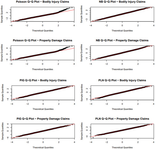
Finally, we fit the univariate NB, PIG, and PLN regression models with varying dispersion for claim frequencies using the univariate version of the EM algorithm presented in Section 2. Additionally, the simple Poisson regression model was fitted for comparison purposes. The normalized randomized quantile residuals (see Dunn and Smyth 1996) are used as a graphical tool to help us assess the adequacy of the fit of the competing models for both bodily injury and property damage claim counts $K_{1,j}$ and $K_{2,j}.$ For these discrete response distributions, the normalized randomized quantile residuals are defined as ${\widehat{r}}_j={\Phi }^{-1}(u_j),$ where ${\Phi }^{-1}$ is the inverse cdf of a standard Normal distribution and where u_j is defined as a random value from the uniform distribution on the interval $\left[F_j({\chi }_j-1|{\mathit{\theta }}^{(r+1)}),F_j({\chi }_j|{\mathit{\theta }}^{(r+1)})\right],$ where F_j is the cdf estimated for the jth individual and where ${\mathit{\theta }}^{(r+1)}$ contains all estimated model parameters after the EM algorithm has reached the global maximum and χ_j is the corresponding observation. The normalized (random) quantiles for the Poisson, NB, PIG, and PLN models are presented in Figure 1 per claim type i = 1, 2. From Figure 1, we observe that the NB, PIG, and PLN are better assumptions than the Poisson model, which does not capture the tails of the claim frequency distributions of $K_{1,j}$ and $K_{2,j}.$ In particular, the residuals of the three mixed Poisson models are close to the diagonal and indicate a good fit to the distributions of both $K_{1,j}$ and $K_{2,j},$ whereas the sample quantiles of the Poisson model, due to the equidispersion constraint, near the tail end of the distributions of both $K_{1,j}$ and $K_{2,j},$ are significantly higher than the theoretical quantiles.

Figure 1. Normalized Quantiles for the Poisson, NB, PIG, and PLN Regression Models with Varying Dispersion.

6.2. Modeling Results

This subsection describes the modeling results of the BNB, BPIG, and BPLN distributions and regression models with varying dispersion.

The ML estimates of their parameters and the corresponding standard errors in parentheses are presented in Table 4 for the distributions⁶ and in Table 5 for the regression models with varying dispersion. Note that in the latter case, for illustrative purposes we considered that the two location parameters ${\mu }_{1,j},{\mu }_{2,j}$ and the dispersion parameter ${\sigma }_j,j=1,\dots ,n,$ of the aforementioned models are modeled using all three available explanatory variables. However, it should be noted that for larger datasets variable selection can start with the examination of the two mean parameters of the bivariate mixed Poisson regression model with varying dispersion. This can be achieved by adding all available covariates and testing whether the exclusion of each one lowers the global deviance (DEV), Akaike information criterion (AIC), and Schwartz Bayesian criterion (SBC) values. Then, after having selected the best predictors for the two mean parameters, we can continue in determining the remaining predictors by testing which rating variable between those used in the two mean parameters would lead to a further decrease of the DEV, AIC, and SBC values when inserted in the dispersion parameter of the bivariate claim frequency model with varying dispersion. Additionally, if between the same bivariate mixed Poisson distribution with different parameter specifications several models have similar DEV, AIC, and SBC values, the simpler model can be used in order to avoid overfitting. Therefore, in such cases, it should be expected that the dispersion parameters of the bivariate mixed Poisson regression model with varying dispersion may have fewer predictors than the two mean parameters.

TABLE 4 Parameters Estimates and Associated Standard Errors of the Fitted BNB, BPIG, and BPLN Distributions

BNB		BPIG		BPLN
μ 1	μ2	μ1	μ2	μ1	μ2
0.0954	0.0618	0.0954	0.0618	0.0954	0.0618
(0.0542)	(0.0639)	(0.0535)	(0.0633)	(0.0546)	(0.0643)
σ		σ		σ
0.2612		0.4866		1.4072
(0.1037)		(0.0554)		(0.0448)

TABLE 5 Parameters Estimates and Associated Standard Errors of the Fitted BNB, BPIG, and BPLN Regression Models with Varying Dispersion for Each Covariate

	BNB			BPIG			BPLN
Variable	Coeff. β1	Coeff. β2	Coeff. β3	Coeff. β1	Coeff. β2	Coeff. β3	Coeff. ${\beta }_1$	Coeff. β2	Coeff. β3
Intercept	–2.3933	–2.9262	–1.1296	–2.3950	–2.9279	–0.5908	–2.3839	–2.9167	0.2380
	(0.0981)	(0.1121)	(0.2126)	(0.0997)	(0.1010)	(0.1418)	(0.0898)	(0.1374)	(0.0474)
v1 C2	0.0524	0.1504	–0.1912	0.0535	0.1518	–0.1157	0.0708	0.1691	0.0905
	(0.0238)	(0.0711)	(0.0940)	(0.0232)	(0.0698)	(0.0564)	(0.0329)	(0.0808)	(0.0436)
v1 C3	0.1556	0.1770	–0.2303	0.1587	0.1793	–0.1364	0.1941	0.2143	0.1223
	(0.0798)	(0.0938)	(0.1268)	(0.0804)	(0.0939)	(0.0732)	(0.1003)	(0.1149)	(0.0685)
v2 C2	0.0452	0.1780	0.3627	0.0465	0.1790	0.1959	0.0348	0.1669	–0.1198
	(0.0169)	(0.0719)	(0.1611)	(0.0170)	(0.0704)	(0.0859)	(0.0137)	(0.0704)	(0.0571)
v3 C2	–0.1216	–0.0203	–0.3144	–0.1203	−0.0190	–0.1769	−0.1000	–0.021	0.1230
	(0.0542)	(0.0093)	(0.1473)	(0.0525)	(0.0085)	(0.0819)	(0.0459)	(0.0098)	(0.0608)
v3 C3	0.1767	0.1712	–0.0883	0.1784	0.1731	–0.0716	0.1934	0.1882	0.0674
	(0.0793)	(0.0786)	(0.0426)	(0.0787)	(0.0776)	(0.0341)	(0.0893)	(0.0895)	(0.0341)

As we can see from Table 5, the values of the estimated regression coefficients of the variables v1, v2, and v3 are almost identical for ${\mu }_{1,j}$ and ${\mu }_{2,j}$ across all three bivariate mixed Poisson distributions, whereas they differ hugely for the dispersion parameter σ_j. Additionally, we observe that the same explanatory variables always have the same effect (positive and/or negative) on the parameter σ_j in the case of the BNB and BPIG models but have a different effect for σ_j in the case of the BPLN model.

6.3. Model Comparison

In this subsection we compare the fit of the BNB, BPIG, and BPLN distributions/regression models with varying dispersion based on the classic hypothesis/specification tests DEV, AIC, and SBC. The DEV is given by (66) $$\text{DEV}=-2\widehat{l}\left(\widehat{\mathit{\theta }}\right),$$(66) with $\widehat{l}$ being the maximum of the log-likelihood and $\widehat{\mathit{\theta }}$ the vector of estimated parameters of the model. Moreover, the AIC is defined as (67) $$\text{AIC}=\text{DEV}+2\times df$$(67) and the SBC is given by (68) $$\text{SBC}=\text{DEV}+\hspace{0.17em}\text{log}\hspace{0.17em}\left(n\right)\times df,$$(68) where df are the degrees of freedom that correspond to the number of fitted parameters in the model and n is the number of observations in the sample. The values of the DEV, AIC, and SBC for the competing bivariate mixed Poisson distributions/regression models with varying dispersion are given in Table 6. According to a very well-known rule of thumb, two models can be considered to be significantly different if the difference in the log-likelihoods exceeds 5, corresponding to a difference in their respective AIC and SBC values of greater than 10 and 5 respectively; see Anderson and Burnham (2004) and Raftery (1995). Therefore, in this case we see that the best fitting performances are provided by the BPIG distribution/regression model with varying dispersion.

TABLE 6 Models Comparison Based on Global Deviance, AIC, and SBC

	Distributions			Regression Models
Model	df	AIC	SBC	Model	df	Global Deviance	AIC	SBC
BNB	3	5615	5635	BNB	18	4388	4424	4542
BPIG	3	5541	5561	BPIG	18	4249	4285	4403
BPLN	3	5684	5704	BPLN	18	4513	4549	4667

6.4. Application to Ratemaking

In this subsection, following the current methodology, as presented in Section 4, we calculate the a posteriori, or bonus-malus, premiums resulting from the three BNB, BPIG, and BPLN distributions/regression models with varying dispersion using the expected value and the variance principles. The premium rates will be divided by the premium when $t=0$––that is, we calculate the relative premiums––because we are interested in the differences between various classes and the results are presented so that the premium for a new policyholder is 100. Thus, in what follows, when the expected value principle is used, note the disappearance of the factor $(1+{\lambda }_1)$ from Equations (52)(52) $$P_1=(1+{\lambda }_1)\frac{{\sigma }_j+\sum _{i=1}^2{k}_{i,j}}{{\sigma }_j+\sum _{l=1}^t\sum _{i=1}^2{\mu }_{i,j,l}}.$$(52) , (53)(53) $$P_1=\frac{(1+{\lambda }_1){\sigma }_j{K}_{\sum _{i=1}^2{k}_{i,j}+\frac{1}{2}}\left({\sigma }_j\sqrt{{\sigma }_j^2+2\sum _{l=1}^t\sum _{i=1}^2{\mu }_{i,j,l}}\right)}{\sqrt{{\sigma }_j^2+2\sum _{l=1}^t\sum _{i=1}^2{\mu }_{i,j,l}}{K}_{\sum _{i=1}^2{k}_{i,j}-\frac{1}{2}}\left({\sigma }_j\sqrt{{\sigma }_j^2+2\sum _{l=1}^t\sum _{i=1}^2{\mu }_{i,j,l}}\right)}.$$(53) , and (54)(54) $$P_1=(1+{\lambda }_1){\int }_0^{\infty }{z}_{j,t+1}\frac{\prod _{l=1}^t\prod _{i=1}^2\frac{\hspace{0.17em}\text{exp}[-({\mu }_{i,j}{z}_j)]{({\mu }_{i,j}{z}_j)}^{k_{i,j}}}{k_{i,j}!}\frac{\hspace{0.17em}\text{exp}[-\frac{{(\hspace{0.17em}\text{log}\hspace{0.17em}(z_{j,t+1})+{\sigma }_j^2/2)}^2}{2{\sigma }_j^2}]}{\sqrt{2\pi }{\sigma }_j{z}_{j,t+1}}}{\underset{0}{\overset{\infty }{\int }}\prod _{i=1}^2\frac{\hspace{0.17em}\text{exp}[-({\mu }_{i,j}{z}_j)]{({\mu }_{i,j}{z}_j)}^{k_{i,j}}}{k_{i,j}!}\frac{\hspace{0.17em}\text{exp}[-\frac{{(\hspace{0.17em}\text{log}\hspace{0.17em}(z_{j,t+1})+{\sigma }_j^2/2)}^2}{2{\sigma }_j^2}]}{\sqrt{2\pi }{\sigma }_j{z}_{j,t+1}}d{z}_{j,t+1}}d{z}_{j,t+1}.$$(54) . Also, when the variance principle is used, following, and extending to the bivariate case the framework of Lemaire (1995) and Tzougas et al. (2018), we consider that ${\lambda }_2=0.235$ in Equations (56)(56) $$P_2=(1+{\lambda }_2)\frac{{\sigma }_j+\sum _{i=1}^2{k}_{i,j}}{{\sigma }_j+\sum _{l=1}^t\sum _{i=1}^2{\mu }_{i,j,l}}+{\lambda }_2\frac{{\sigma }_j+\sum _{i=1}^2{k}_{i,j}}{{({\sigma }_j+\sum _{l=1}^t\sum _{i=1}^2{\mu }_{i,j,l})}^2}.$$(56) , (57)(57) $$\begin{array}{c}{P}_2=\frac{(1+{\lambda }_2){\sigma }_j{K}_{\sum _{i=1}^2{k}_{i,j}+\frac{1}{2}}({\sigma }_j\sqrt{{\sigma }_j^2+2\sum _{l=1}^t\sum _{i=1}^2{\mu }_{i,j,l}})}{\sqrt{{\sigma }_j^2+2\sum _{l=1}^t\sum _{i=1}^2{\mu }_{i,j,l}}{K}_{\sum _{i=1}^2{k}_{i,j}-\frac{1}{2}}({\sigma }_j\sqrt{{\sigma }_j^2+2\sum _{l=1}^t\sum _{i=1}^2{\mu }_{i,j,l}})}\hfill \\ +{\lambda }_2(\frac{{\sigma }_j^2}{{\sigma }_j^2+2\sum _{l=1}^t\sum _{i=1}^2{\mu }_{i,j,l}})[\frac{K_{\sum _{i=1}^2{k}_{i,j}+\frac{3}{2}}({\sigma }_j\sqrt{{\sigma }_j^2+2\sum _{l=1}^t\sum _{i=1}^2{\mu }_{i,j,l}})}{K_{\sum _{i=1}^2{k}_{i,j}-\frac{1}{2}}({\sigma }_j\sqrt{{\sigma }_j^2+2\sum _{l=1}^t\sum _{i=1}^2{\mu }_{i,j,l}})}\hfill \\ -{(\frac{K_{\sum _{i=1}^2{k}_{i,j}+\frac{1}{2}}({\sigma }_j\sqrt{{\sigma }_j^2+2\sum _{l=1}^t\sum _{i=1}^2{\mu }_{i,j,l}})}{K_{\sum _{i=1}^2{k}_{i,j}-\frac{1}{2}}({\sigma }_j\sqrt{{\sigma }_j^2+2\sum _{l=1}^t\sum _{i=1}^2{\mu }_{i,j,l}})})}^2].\hfill \end{array}$$(57) , and (58)(58) $$\begin{array}{c}{P}_2=(1+{\lambda }_2){\int }_0^{\infty }{z}_{j,t+1}\frac{\prod _{l=1}^t\prod _{i=1}^2\frac{\hspace{0.17em}\text{exp}[-({\mu }_{i,j}{z}_j)]{({\mu }_{i,j}{z}_j)}^{k_{i,j}}}{k_{i,j}!}\frac{\hspace{0.17em}\text{exp}[-\frac{{(\hspace{0.17em}\text{log}\hspace{0.17em}(z_{j,t+1})+{\sigma }_j^2/2)}^2}{2{\sigma }_j^2}]}{\sqrt{2\pi }{\sigma }_j{z}_{j,t+1}}}{\underset{0}{\overset{\infty }{\int }}\prod _{i=1}^2\frac{\hspace{0.17em}\text{exp}[-({\mu }_{i,j}{z}_j)]{({\mu }_{i,j}{z}_j)}^{k_{i,j}}}{k_{i,j}!}\frac{\hspace{0.17em}\text{exp}[-\frac{{(\hspace{0.17em}\text{log}\hspace{0.17em}(z_{j,t+1})+{\sigma }_j^2/2)}^2}{2{\sigma }_j^2}]}{\sqrt{2\pi }{\sigma }_j{z}_{j,t+1}}d{z}_{j,t+1}}d{z}_{j,t+1}\\ +{\lambda }_2[{\int }_0^{\infty }{z}_{j,t+1}^2\frac{\prod _{l=1}^t\prod _{i=1}^2\frac{\hspace{0.17em}\text{exp}[-({\mu }_{i,j}{z}_j)]{({\mu }_{i,j}{z}_j)}^{k_{i,j}}}{k_{i,j}!}\frac{\hspace{0.17em}\text{exp}[-\frac{{(\hspace{0.17em}\text{log}\hspace{0.17em}(z_{j,t+1})+{\sigma }_j^2/2)}^2}{2{\sigma }_j^2}]}{\sqrt{2\pi }{\sigma }_j{z}_{j,t+1}}}{\underset{0}{\overset{\infty }{\int }}\prod _{i=1}^2\frac{\hspace{0.17em}\text{exp}[-({\mu }_{i,j}{z}_j)]{({\mu }_{i,j}{z}_j)}^{k_{i,j}}}{k_{i,j}!}\frac{\hspace{0.17em}\text{exp}[-\frac{{(\hspace{0.17em}\text{log}\hspace{0.17em}(z_{j,t+1})+{\sigma }_j^2/2)}^2}{2{\sigma }_j^2}]}{\sqrt{2\pi }{\sigma }_j{z}_{j,t+1}}d{z}_{j,t+1}}d{z}_{j,t+1}\\ -{({\int }_0^{\infty }{z}_{j,t+1}\frac{\prod _{l=1}^t\prod _{i=1}^2\frac{\hspace{0.17em}\text{exp}[-({\mu }_{i,j}{z}_j)]{({\mu }_{i,j}{z}_j)}^{k_{i,j}}}{k_{i,j}!}\frac{\hspace{0.17em}\text{exp}[-\frac{{(\hspace{0.17em}\text{log}\hspace{0.17em}(z_{j,t+1})+{\sigma }_j^2/2)}^2}{2{\sigma }_j^2}]}{\sqrt{2\pi }{\sigma }_j{z}_{j,t+1}}}{\underset{0}{\overset{\infty }{\int }}\prod _{i=1}^2\frac{\hspace{0.17em}\text{exp}[-({\mu }_{i,j}{z}_j)]{({\mu }_{i,j}{z}_j)}^{k_{i,j}}}{k_{i,j}!}\frac{\hspace{0.17em}\text{exp}[-\frac{{(\hspace{0.17em}\text{log}\hspace{0.17em}(z_{j,t+1})+{\sigma }_j^2/2)}^2}{2{\sigma }_j^2}]}{\sqrt{2\pi }{\sigma }_j{z}_{j,t+1}}d{z}_{j,t+1}}d{z}_{j,t+1})}^2].\end{array}$$(58) , which corresponds to a safety loading of 25% of the net premium.

Firstly, assuming that the number of individual bodily injury and property damage claims, $K_{1,j}$ and $K_{2,j},$ respectively, with $j=1,\dots ,n,$ ranges from 0 to 3 and the age of the policy is t = 1, t = 2, and t = 3 years, we computed comparable relative premiums for the three bivariate mixed Poisson distributions. Tables 7 and 8 present the premium rates calculated according to the expected value and variance principles, respectively.

TABLE 7 Comparison of the A Posteriori, or Bonus–Malus, Premium Rates for $t=1,2,3,$ Bivariate Claim Frequency Distributions under the Expected Value Principle

	t = 1				t = 1				t = 1
	BNB distribution				BPIG distribution				BPLN distribution
$k_{1,j}/k_{2,j}$	0	1	2	3	0	1	2	3	0	1	2	3
$0$	72.69	350.98	629.27	907.56	79.80	256.06	553.66	892.83	81.47	244.10	510.00	847.30
$1$	350.98	629.27	907.56	1185.85	256.06	553.66	892.83	1240.99	244.10	510.00	847.30	1227.45
$2$	629.27	907.56	1185.85	1464.14	553.66	892.83	1240.99	1591.52	510.00	847.30	1227.45	1633.51
$3$	907.56	1185.85	1464.14	1742.43	892.83	1240.99	1591.52	1942.92	847.30	1227.45	1633.51	2056.12
	t = 2				t = 2				t = 2
	BNB distribution				BPIG distribution				BPLN distribution
$k_{1,j}/k_{2,j}$	0	1	2	3	0	1	2	3	0	1	2	3
0	57.10	275.69	494.28	712.87	68.35	197.65	411.53	657.85	70.44	193.99	382.91	614.90
1	275.69	494.28	712.87	931.46	197.65	411.53	657.85	912.20	193.99	382.91	614.90	872.58
2	494.28	712.87	931.46	1150.05	411.53	657.85	912.20	1168.82	382.91	614.90	872.58	1145.94
3	712.87	931.46	1150.05	1368.64	657.85	912.20	1168.82	1426.30	614.90	872.58	1145.94	1429.44
	t = 3				t = 3				t = 3
	BNB distribution				BPIG distribution				BPLN distribution
$k_{1,j}/k_{2,j}$	0	1	2	3	0	1	2	3	0	1	2	3
0	47.01	226.99	406.97	586.96	60.73	162.83	328.94	521.70	62.81	163.41	310.83	488.29
1	226.99	406.97	586.96	766.94	162.83	328.94	521.70	721.75	163.41	310.83	488.29	683.62
2	406.97	586.96	766.94	946.92	328.94	521.70	721.75	923.98	310.83	488.29	683.62	889.94
3	586.96	766.94	946.92	1126.90	521.70	721.75	923.98	1127.06	488.29	683.62	889.94	1103.44

TABLE 8 Comparison of the A Posteriori, or Bonus–Malus, Premium Rates for $t=1,2,3,$ Bivariate Claim Frequency Distributions under the Variance Principle

	t = 1				t = 1				t = 1
	BNB distribution				BPIG distribution				BPLN distribution
$k_{1,j}/k_{2,j}$	0	1	2	3	0	1	2	3	0	1	2	3
$0$	66.48	321.01	575.54	830.07	72.36	261.00	585.67	951.89	74.79	248.08	553.01	953.33
$1$	321.01	575.54	830.07	1084.61	261.00	585.67	951.89	1325.81	248.08	553.01	953.33	1411.35
$2$	575.54	830.07	1084.61	1339.14	585.67	951.89	1325.81	1701.58	553.01	953.33	1411.35	1903.99
$3$	830.07	1084.61	1339.14	1593.67	951.89	1325.81	1701.58	2078.02	953.33	1411.35	1903.99	2418.52
	t = 2				t = 2				t = 2
	BNB distribution				BPIG distribution				BPLN distribution
$k_{1,j}/k_{2,j}$	0	1	2	3	0	1	2	3	0	1	2	3
0	49.44	238.71	427.98	617.26	59.00	186.12	399.90	644.15	62.04	182.94	376.80	620.13
1	238.71	427.98	617.26	806.53	186.12	399.90	644.15	895.13	182.94	376.80	620.13	893.03
2	427.98	617.26	806.53	995.80	399.90	644.15	895.13	1147.87	376.80	620.13	893.03	1183.86
3	617.26	806.53	995.80	1185.08	644.15	895.13	1147.87	1401.27	620.13	893.03	1183.86	1486.19
	t = 3				t = 3				t = 3
	BNB distribution				BPIG distribution				BPLN distribution
$k_{1,j}/k_{2,j}$	0	1	2	3	0	1	2	3	0	1	2	3
0	39.22	189.39	339.56	489.73	50.89	146.12	303.31	484.57	53.94	147.64	289.72	463.44
1	189.39	339.56	489.73	639.89	146.12	303.31	484.57	671.85	147.64	289.72	463.44	655.99
2	339.56	489.73	639.89	790.06	303.31	484.57	671.85	860.82	289.72	463.44	655.99	860.06
3	489.73	639.89	790.06	940.23	484.57	671.85	860.82	1050.43	463.44	655.99	860.06	1071.59

Secondly, when both the a posteriori and the a priori criteria––that is the characteristics of the policyholders and their cars––are considered, we analyze three risk class profiles that we classify as best, average, and worst according to the values of the mean claim frequencies ${\mu }_{1,j}$ and ${\mu }_{2,j},$ which are calculated using the same set of explanatory variables per claim type i = 1, 2 in the case of the BNB, BPIG, and BPLN models, respectively. More specifically, for our data, we characterize the best, average, and worst profiles as such based on category C1 for all three explanatory variables v1, v2, and v3 in the case of the first; category C2 for v1, v2, and v3 in the case of the second; and category C3 for v1 and v3 and C2 for v2 in the case of the third. Also, the dispersion parameter ${\sigma }_j$ of the BNB, BPIG, and BPLN models is computed for each risk class profile. The results are shown in Table 9.

Table 9 Results of the Fitted BNB, BPIG, and BPLN Regression Models with Varying Dispersion for Each Risk Class Profile

Regression model	Profile	${\mu }_{1,j}$	Profile	${\mu }_{2,j}$	Profile	σj
	Best	0.09132733	Best	0.05359886	Best	0.3231537
BNB	Average	0.0891615	Average	0.07294194	Average	0.2801163
	Worst	0.133208	Worst	0.09072674	Worst	0.3377262
	Best	0.09117268	Best	0.05350929	Best	0.553884
BPIG	Average	0.08934053	Average	0.07308735	Average	0.5028316
	Worst	0.1338012	Worst	0.09103602	Worst	0.5472224
	Best	0.09219446	Best	0.05411198	Best	1.268773
BPLN	Average	0.09270516	Average	0.07414734	Average	1.393263
	Worst	0.1406319	Worst	0.09563929	Worst	1.360708

From Table 9 we observe that for all three risk profiles small differences lie in the mean values ${\mu }_{1,j}$ and ${\mu }_{2,j}$ of the BNB, BPG, and BPLN models. On the contrary, as previously mentioned, more significant differences are noticed across the three risk profiles in the values of the dispersion parameters σ_j of the bivariate mixed Poisson models. Due to these discrepancies, the a posteriori, or bonus-malus, premium rates that will result from the three models by updating their posterior mean and the posterior variance will be better distinguished under different distributional assumptions. Thus, as was previously mentioned, the proposed modeling framework leads to a better tariffication than the assumption of a constant dispersion σ_j.

In what follows, Tables 10, 11, and 12 depict the premiums computed under the expected value principle for the three risk profiles during the years t = 1, t = 2, and t = 3 respectively. Furthermore, Tables 13, 14, and 15 present the premiums calculated via the variance principle for the same risk profiles and years of insurance policy.

TABLE 10 Comparison of the A Posteriori, or Bonus–Malus, Premium Rates for t = 1 under the Expected Value Principle, Bivariate Claim Frequency Regression Models with Varying Dispersion

	t = 1				t = 1				t = 1
	BNB regression model				BPIG regression model				BPLN regression model
	Best profile				Best profile				Best profile
$k_{1,j}/k_{2,j}$	0	1	2	3	0	1	2	3	0	1	2	3
$0$	76.36	312.65	548.94	785.23	82.05	239.47	500.38	800.56	83.78	223.13	451.24	749.12
$1$	312.65	548.94	785.23	1021.52	239.47	500.38	800.56	1110.36	223.13	451.24	749.12	1093.54
$2$	548.94	785.23	1021.52	1257.81	500.38	800.56	1110.36	1422.85	451.24	749.12	1093.54	1467.98
$3$	785.23	1021.52	1257.81	1494.10	800.56	1110.36	1422.85	1736.37	749.12	1093.54	1467.98	1862.30
	t = 1				t = 1				t = 1
	BNB regression model				BPIG regression model				BPLN regression model
	Average profile				Average profile				Average profile
$k_{1,j}/k_{2,j}$	0	1	2	3	0	1	2	3	0	1	2	3
0	73.18	334.41	595.64	856.88	80.00	247.48	528.29	849.50	81.26	237.30	489.54	808.55
1	334.41	595.64	856.88	1118.11	247.48	528.29	849.50	1179.87	237.30	489.54	808.55	1167.96
2	595.64	856.88	1118.11	1379.35	528.29	849.50	1179.87	1512.72	489.54	808.55	1167.96	1551.97
3	856.88	1118.11	1379.35	1640.58	849.50	1179.87	1512.72	1846.48	808.55	1167.96	1551.97	1951.77
	t = 1				t = 1				t = 1
	BNB regression model				BPIG regression model				BPLN regression model
	Worst profile				Worst profile				Worst profile
$k_{1,j}/k_{2,j}$	0	1	2	3	0	1	2	3	0	1	2	3
0	71.49	283.19	494.88	706.58	79.05	210.99	425.43	674.37	79.41	209.86	408.55	653.84
1	283.19	494.88	706.58	918.27	210.99	425.43	674.37	932.83	209.86	408.55	653.84	927.77
2	494.88	706.58	918.27	1129.97	425.43	674.37	932.83	1194.13	408.55	653.84	927.77	1219.52
3	706.58	918.27	1129.97	1341.66	674.37	932.83	1194.13	1456.54	653.84	927.77	1219.52	1522.90

TABLE 11 Comparison of the A Posteriori, or Bonus–Malus, Premium Rates for t = 2 under the Expected Value Principle, Bivariate Claim Frequency Regression Models with Varying Dispersion

	t = 2				t = 2				t = 2
	BNB regression model				BPIG regression model				BPLN regression model
	Best profile				Best profile				Best profile
$k_{1,j}/k_{2,j}$	0	1	2	3	0	1	2	3	0	1	2	3
$0$	61.76	252.87	443.97	635.08	71.23	189.88	382.67	606.51	73.58	181.78	347.13	554.85
$1$	252.87	443.97	635.08	826.19	189.88	382.67	606.51	838.91	181.78	347.13	554.85	790.34
$2$	443.97	635.08	826.19	1017.30	382.67	606.51	838.91	1073.89	347.13	554.85	790.34	1043.81
$3$	635.08	826.19	1017.30	1208.41	606.51	838.91	1073.89	1309.87	554.85	790.34	1043.81	1309.31
	t = 2				t = 2				t = 2
	BNB regression model				BPIG regression model				BPLN regression model
	Average profile				Average profile				Average profile
$k_{1,j}/k_{2,j}$	0	1	2	3	0	1	2	3	0	1	2	3
0	57.70	263.68	469.66	675.64	68.60	191.76	394.00	627.70	70.14	188.56	367.80	587.30
1	263.68	469.66	675.64	881.63	191.76	394.00	627.70	869.56	188.56	367.80	587.30	831.00
2	469.66	675.64	881.63	1087.61	394.00	627.70	869.56	1113.77	367.80	587.30	831.00	1089.59
3	675.64	881.63	1087.61	1293.59	627.70	869.56	1113.77	1358.89	587.30	831.00	1089.59	1357.84
	t = 2				t = 2				t = 2
	BNB regression model				BPIG regression model				BPLN regression model
	Worst profile				Worst profile				Worst profile
$k_{1,j}/k_{2,j}$	0	1	2	3	0	1	2	3	0	1	2	3
0	55.64	220.37	385.11	549.85	67.41	163.36	315.66	494.13	67.61	165.48	306.02	474.57
1	220.37	385.11	549.85	714.58	163.36	315.66	494.13	680.83	165.48	306.02	474.57	660.27
2	385.11	549.85	714.58	879.32	315.66	494.13	680.83	870.20	306.02	474.57	660.27	856.74
3	549.85	714.58	879.32	1044.06	494.13	680.83	870.20	1060.64	474.57	660.27	856.74	1060.34

TABLE 12 Comparison of the A Posteriori, or Bonus–Malus, Premium Rates for t = 3 under the Expected Value Principle, Bivariate Claim Frequency Regression Models with Varying Dispersion

	t = 3				t = 3				t = 3
	BNB regression model				BPIG regression model				BPLN regression model
	Best profile				Best profile				Best profile
$k_{1,j}/k_{2,j}$	0	1	2	3	0	1	2	3	0	1	2	3
$0$	51.84	212.28	372.71	533.14	63.81	159.01	311.21	489.09	66.31	155.60	286.21	446.43
$1$	212.28	372.71	533.14	693.57	159.01	311.21	489.09	674.74	155.60	286.21	446.43	625.90
$2$	372.71	533.14	693.57	854.00	311.21	489.09	674.74	862.85	286.21	446.43	625.90	817.88
$3$	533.14	693.57	854.00	1014.44	489.09	674.74	862.85	1051.94	446.43	625.90	817.88	1018.29
	t = 3				t = 3				t = 3
	BNB regression model				BPIG regression model				BPLN regression model
	Average profile				Average profile				Average profile
$k_{1,j}/k_{2,j}$	0	1	2	3	0	1	2	3	0	1	2	3
0	47.63	217.65	387.67	557.69	61.01	158.38	315.63	498.68	62.47	158.82	298.70	466.63
1	217.65	387.67	557.69	727.71	158.38	315.63	498.68	689.11	158.82	298.70	466.63	651.41
2	387.67	557.69	727.71	897.73	315.63	498.68	689.11	881.80	298.70	466.63	651.41	846.62
3	557.69	727.71	897.73	1067.75	498.68	689.11	881.80	1075.38	466.63	651.41	846.62	1048.66
	t = 3				t = 3				t = 3
	BNB regression model				BPIG regression model				BPLN regression model
	Worst profile				Worst profile				Worst profile
$k_{1,j}/k_{2,j}$	0	1	2	3	0	1	2	3	0	1	2	3
0	45.54	180.36	315.19	450.02	59.75	135.14	252.57	391.05	59.64	138.67	248.03	376.88
1	180.36	315.19	450.02	584.85	135.14	252.57	391.05	536.82	138.67	248.03	376.88	517.66
2	315.19	450.02	584.85	719.68	252.57	391.05	536.82	685.10	248.03	376.88	517.66	665.98
3	450.02	584.85	719.68	854.51	391.05	536.82	685.10	834.43	376.88	517.66	665.98	819.34

TABLE 13 Comparison of the A Posteriori, or Bonus–Malus, Premium Rates for t = 1 under the Variance Principle, Bivariate Claim Frequency Regression Models with Varying Dispersion

	t = 1				t = 1				t = 1
	BNB regression model				BPIG regression model				BPLN regression model
	Best profile				Best profile				Best profile
$k_{1,j}/k_{2,j}$	0	1	2	3	0	1	2	3	0	1	2	3
$0$	71.14	291.28	511.43	731.57	75.56	246.18	534.73	863.49	77.96	228.96	496.95	862.56
$1$	291.28	511.43	731.57	951.72	246.18	534.73	863.49	1200.74	228.96	496.95	862.56	1294.49
$2$	511.43	731.57	951.72	1171.86	534.73	863.49	1200.74	1540.17	496.95	862.56	1294.49	1769.17
$3$	731.57	951.72	1171.86	1392.01	863.49	1200.74	1540.17	1880.38	862.56	1294.49	1769.17	2271.92
	t = 1				t = 1				t = 1
	BNB regression model				BPIG regression model				BPLN regression model
	Average profile				Average profile				Average profile
$k_{1,j}/k_{2,j}$	0	1	2	3	0	1	2	3	0	1	2	3
0	67.27	307.42	547.58	787.73	72.87	251.97	558.09	904.78	74.80	240.29	526.97	901.62
1	307.42	547.58	787.73	1027.88	251.97	558.09	904.78	1259.41	240.29	526.97	901.62	1329.89
2	547.58	787.73	1027.88	1268.04	558.09	904.78	1259.41	1616.01	526.97	901.62	1329.89	1790.58
3	787.73	1027.88	1268.04	1508.19	904.78	1259.41	1616.01	1973.31	901.62	1329.89	1790.58	2271.89
	t = 1				t = 1				t = 1
	BNB regression model				BPIG regression model				BPLN regression model
	Worst profile				Worst profile				Worst profile
$k_{1,j}/k_{2,j}$	0	1	2	3	0	1	2	3	0	1	2	3
0	66.34	262.76	459.19	655.61	73.04	211.66	440.86	704.99	73.95	208.77	424.18	696.33
1	262.76	459.19	655.61	852.04	211.66	440.86	704.99	977.73	208.77	424.18	696.33	1003.48
2	459.19	655.61	852.04	1048.46	440.86	704.99	977.73	1252.87	424.18	696.33	1003.48	1332.26
3	655.61	852.04	1048.46	1244.89	704.99	977.73	1252.87	1528.92	696.33	1003.48	1332.26	1675.09

TABLE 14 Comparison of the A Posteriori, or Bonus–Malus, Premium Rates for t = 2 under the Variance Principle, Bivariate Claim Frequency Regression Models with Varying Dispersion

	t = 2				t = 2				t = 2
	BNB regression model				BPIG regression model				BPLN regression model
	Best profile				Best profile				Best profile
$k_{1,j}/k_{2,j}$	0	1	2	3	0	1	2	3	0	1	2	3
$0$	54.93	224.92	394.90	564.89	62.74	181.82	378.71	605.61	66.00	174.25	348.58	573.77
$1$	224.92	394.90	564.89	734.87	181.82	378.71	605.61	839.91	174.25	348.58	573.77	832.60
$2$	394.90	564.89	734.87	904.86	378.71	605.61	839.91	1076.28	348.58	573.77	832.60	1113.15
$3$	564.89	734.87	904.86	1074.84	605.61	839.91	1076.28	1313.42	573.77	832.60	1113.15	1408.11
	t = 2				t = 2				t = 2
	BNB regression model				BPIG regression model				BPLN regression model
	Average profile				Average profile				Average profile
$k_{1,j}/k_{2,j}$	0	1	2	3	0	1	2	3	0	1	2	3
0	50.36	230.12	409.89	589.66	59.61	180.97	383.57	615.93	62.05	177.77	360.91	589.90
1	230.12	409.89	589.66	769.43	180.97	383.57	615.93	855.20	177.77	360.91	589.90	846.51
2	409.89	589.66	769.43	949.20	383.57	615.93	855.20	1096.33	360.91	589.90	846.51	1120.00
3	589.66	769.43	949.20	1128.97	615.93	855.20	1096.33	1338.15	589.90	846.51	1120.00	1404.37
	t = 2				t = 2				t = 2
	BNB regression model				BPIG regression model				BPLN regression model
	Worst profile				Worst profile				Worst profile
$k_{1,j}/k_{2,j}$	0	1	2	3	0	1	2	3	0	1	2	3
0	49.39	195.63	341.87	488.12	59.96	154.14	305.77	482.55	60.91	155.65	295.83	466.36
1	195.63	341.87	488.12	634.36	154.14	305.77	482.55	666.61	155.65	295.83	466.36	655.49
2	341.87	488.12	634.36	780.60	305.77	482.55	666.61	852.92	295.83	466.36	655.49	856.22
3	488.12	634.36	780.60	926.84	482.55	666.61	852.92	1040.11	466.36	655.49	856.22	1064.60

TABLE 15 Comparison of the A Posteriori, or Bonus–Malus, Premium Rates for t = 3 under the Variance Principle, Bivariate Claim Frequency Regression Models with Varying Dispersion

	t = 3				t = 3				t = 3
	BNB regression model				BPIG regression model				BPLN regression model
	Best profile				Best profile				Best profile
$k_{1,j}/k_{2,j}$	0	1	2	3	0	1	2	3	0	1	2	3
$0$	44.63	182.73	320.83	458.94	54.65	145.58	293.19	464.71	58.13	143.33	272.77	434.72
$1$	182.73	320.83	458.94	597.04	145.58	293.19	464.71	642.82	143.33	272.77	434.72	617.91
$2$	320.83	458.94	597.04	735.14	293.19	464.71	642.82	822.90	272.77	434.72	617.91	814.87
$3$	458.94	597.04	735.14	873.25	464.71	642.82	822.90	1003.75	434.72	617.91	814.87	1021.05
	t = 3				t = 3				t = 3
	BNB regression model				BPIG regression model				BPLN regression model
	Average profile				Average profile				Average profile
$k_{1,j}/k_{2,j}$	0	1	2	3	0	1	2	3	0	1	2	3
0	40.12	183.35	326.59	469.82	51.52	142.72	292.14	465.05	53.94	143.75	278.37	442.40
1	183.35	326.59	469.82	613.05	142.72	292.14	465.05	644.11	143.75	278.37	442.40	624.08
2	326.59	469.82	613.05	756.28	292.14	465.05	644.11	824.96	278.37	442.40	624.08	816.63
3	469.82	613.05	756.28	899.52	465.05	644.11	824.96	1006.48	442.40	624.08	816.63	1016.26
	t = 3				t = 3				t = 3
	BNB regression model				BPIG regression model				BPLN regression model
	Worst profile				Worst profile				Worst profile
$k_{1,j}/k_{2,j}$	0	1	2	3	0	1	2	3	0	1	2	3
0	39.26	155.51	271.75	388.00	51.97	122.99	234.97	366.53	52.68	126.40	230.59	354.57
1	155.51	271.75	388.00	504.24	122.99	234.97	366.53	504.45	126.40	230.59	354.57	490.66
2	271.75	388.00	504.24	620.49	234.97	366.53	504.45	644.48	230.59	354.57	490.66	634.38
3	388.00	504.24	620.49	736.73	366.53	504.45	644.48	785.36	354.57	490.66	634.38	783.16

We make the following observations regarding the results presented in Tables 7, 8, and 10–15.

• Firstly, we see that if the policyholder j has a claim-free year, the premium rates reduce, whereas if they have one or more claims, the premium rates increase, resulting in bonus or malus, respectively.

  • For example, for the case when the expected value principle is used, we observe from Table 7 that a claim-free year for both types of claims i = 1, 2 the policyholder will receive bonuses of 27.31%, 20.20% and 18.53% in year $t=1$ in the case of the BNB, BPIG, and BPLN distributions, respectively. Furthermore, the insureds who had $k_{1,j}=2$ and $k_{2,j}=1$ claims in year t = 1 will have to pay a malus of 807.56%, 792.83%, and 747.30% in the case of the BNB, BPIG, and BPLN distributions, respectively. Regarding the case with covariates, we see from Table 12 that claim free individuals per claim-type i = 1, 2 in year t = 3 will receive bonuses of 48.16%, 36.19%, and 33.69% with the best profile, 52.37%, 38.99%, and 37.53% with the average profile, and 54.46%, 40.25%, and 40.36% with the worst profile in the case of the BNB, BPIG, and BPLN regression models with varying dispersion, respectively. Additionally, we see from Table 12 that policyholders who had $k_{1,j}=2$ and $k_{2,j}=1$ claims in year t = 3 will have to pay maluses of 433.14%, 389.09%, and 346.43% with the best profile, 457.69%, 398.68%, and 366.63% with the average profile. and 350.02%, 291.05%, and 276.88% with the worst profile in the case of the BNB, BPIG, and BPLN regression models with varying dispersion, respectively.

  • Similarly, for the case when the variance principle is used, we observe from Table 8 that a claim-free individual for both types of claims i = 1, 2 insured will receive a bonus of 60.78%, 49.11%, and 46.06% in year t = 3 in the case of the BNB, BPIG, and BPLN distributions, respectively. Also, individuals who had $k_{1,j}=2$ and $k_{2,j}=3$ claims in year t = 3 will have to pay a malus of 690.06%, 760.82%, and 760.06% in the case of the BNB, BPIG, and BPLN distributions, respectively. Regarding the case with covariates, we see from Table 14 that claim-free insureds per claim type i = 1, 2 in year t = 2 will receive bonuses of 45.07%, 37.26%, and 34.00% with the best profile, 49.64%, 40.39%, and 37.95% with the average profile, 50.61%, 40.04%, and 39.09% with the worst profile in the case of the BNB, BPIG, and BPLN regression models with varying dispersion, respectively. Furthermore, we see from Table 14 that policyholders who had $k_{1,j}=2$ and $k_{2,j}=3$ claims in year t = 2 will have to pay a malus of 804.86%, 976.28%, and 1013.15% with the best profile; 849.20%, 996.33%, and 1020.00% with the average profile; and 680.60%, 752.92%, and 756.22% with the worst profile in the case of the BNB, BPIG, and BPLN regression models with varying dispersion, respectively.

• Secondly, regarding the premiums resulting from the same bivariate mixed Poisson distribution/regression model with varying dispersions, we see that

  • For the cases without and with covariates, the use of the variance principle results in higher bonuses for claim-free policyholders than those that are awarded to them using the expected value principle.

  • For the case with covariates, as we can see from Tables 10–15, the proposed modeling framework encourages good driving behavior in two ways:

  1. The bonuses that are awarded to claim-free policyholders with higher risk profiles are slightly higher than those that are awarded to claim-free insureds with lower risk profiles.

  2. The maluses that should be paid by policyholders who had at least one bodily injury and/or property damage claim are slightly lower if they have a higher risk profile.

• Finally, it is worth noting that Tables 10–15 provide a more complete picture to the insurance company than Tables 7 and 8 of when only the a posteriori criteria were considered, because all of the important a priori and a posteriori information for the number of bodily injury and property damage claims, $K_{1,j}$ and $K_{2,j}$ respectively, of policyholder j is considered in order to estimate their risk of having an accident and thus they permit the differentiation of the a posteriori, or bonus-malus, premiums for various number of bodily injury and property damage claims by updating the posterior mean and the posterior variance based on all available information on the level of riskiness of this individual.

6.5. The Simulated Data

In this subsection, we demonstrate the flexibility of the copula-based model discussed in Section 5 for taking into account the effect of policyholder and coverage type covariates on the mean, dispersion, and dependence components.

For illustrative purposes, the Normal copula will be paired with two NB Type I (NBI), or Poisson–Gamma, distributions.⁷ Then, the jpmf of the Normal copula-based NB regression model with varying dispersion and dependence can be obtained using Equation (59)(59) $$\begin{array}{cc}h(k_{1,j},k_{2,j};{\mu }_{1,j},{\sigma }_{1,j},{\mu }_{2,j},{\sigma }_{2,j})\hfill & =C_{{\theta }_j}(F_1(K_{1,j};{\mu }_{1,j},{\sigma }_{1,j}),F_2(K_{2,j};{\mu }_{2,j},{\sigma }_{2,j}))\hfill \\ -C_{{\theta }_j}(F_1(K_{1,j}-1;{\mu }_{1,j},{\sigma }_{1,j}),F_2(K_{2,j};{\mu }_{2,j},{\sigma }_{2,j}))\hfill \\ -C_{{\theta }_j}(F_1(K_{1,j};{\mu }_{1,j},{\sigma }_{1,j}),F_2(K_{2,j}-1;{\mu }_{2,j},{\sigma }_{2,j}))\hfill \\ +C_{{\theta }_j}(F_1(K_{1,j}-1;{\mu }_{1,j},{\sigma }_{1,j}),F_2(K_{2,j}-1;{\mu }_{2,j},{\sigma }_{2,j})).\hfill \end{array}$$(59) .

A dataset of size n = 20,000 was randomly generated from the bivariate normal copula with two univariate NBI regression models with varying dispersion and we assumed that the two response variables $K_{1,j}$ and $K_{2,j}$ represent claim frequencies for two types of claims, Type I and Type II, from different types of coverage. Furthermore, we considered that the explanatory variables v1–v5 influence the mean, dispersion, and copula parameters. In particular, we assumed that v1 is continuous and it can take integer values between 18 and 75 and v2–v5 are discrete, with v2, v4, and v5 having two categories each and v3 having three categories. Furthermore, we included v1, v2, v3, and v4 in Equations (61)(61) $${\mu }_{1,j}=\hspace{0.17em}\text{exp}\hspace{0.17em}\left({\mathit{x}}_{\mathit{1},\mathit{j}}{}^T{\mathit{\beta }}_{\mathit{1}}\right),$$(61) and (63)(63) $${\sigma }_{1,j}=\hspace{0.17em}\text{exp}\hspace{0.17em}\left({\mathit{x}}_{\mathit{3},\mathit{j}}{}^T{\mathit{\beta }}_{\mathit{3}}\right),$$(63) to explain the mean and dispersion of Type I claims and v1, v2, v3, and v5 in Equations (62)(62) $${\mu }_{2,j}=\hspace{0.17em}\text{exp}\hspace{0.17em}\left({\mathit{x}}_{\mathit{2},\mathit{j}}{}^T{\mathit{\beta }}_{\mathit{2}}\right),$$(62) and (64)(64) $${\sigma }_{2,j}=\hspace{0.17em}\text{exp}\hspace{0.17em}\left({\mathit{x}}_{\mathit{4},\mathit{j}}{}^T{\mathit{\beta }}_{\mathit{4}}\right),\mathrm{ }\text{and}$$(64) to explain the mean and dispersion of Type II claims. Finally, we selected the common variables v1–v3 in Equation (65)(65) $${\theta }_j=\frac{2}{\pi }\arctan \left({\mathit{x}}_{\mathit{5},\mathit{j}}{}^T{\mathit{\beta }}_{\mathit{5}}\right),$$(65) to explain the dependence heterogeneity between two coverages.

The bivariate Normal copula-based NB regression model with varying dispersion and dependence is fitted on these data and the results⁸ are presented in Table 16.

TABLE 16 Normal Copula-Based NB Regression Model with Varying Dispersion and Dependence

	Estimation Results
Variable	Coeff. β 1	Coeff. β2	Coeff. β3	Coeff. β4	Coeff. β5
Intercept	–2.8489	–2.4153	2.7503	2.7006	0.0831
v1	–0.0023	0.0063	–0.0060	0.0003	0.0112
v2 C2	–0.0461	–0.0899	0.5459	–0.0438	0.0910
v3 C2	0.3603	0.0258	–0.7242	–0.1279	0.1526
v3 C3	0.0309	–0.1396	–0.8426	–0.0277	0.1255
v4 C2	–0.1214	––	0.6805	––	––
v4 C3	–0.0262	––	0.0797	––	––
v5 C2	––	0.2281	––	0.2688	–

6.6. Computational Aspects

This subsection discusses the computational issues related to the implementation of the EM algorithm for the BNB, BPIG, and BPLN regression models with varying dispersion and the standard ML estimation method used for the Normal copula-based NB regression model with varying dispersion and dependence. All computing was done using the programming language R (R Core Team 2021).

Regarding the EM estimation procedure for the BNB, BPIG, and BPLN regression models, it should be noted that a rather strict criterion was used and it took the algorithm, for cases both with and without covariate information, a quite large number of iterations to converge. In particular, the stopping criterion was set as $\mathit{tol}={10}^{-12}.$ The standard errors of the BNB, BPIG, and BPLN regression models with varying dispersion were obtained using the standard approach of Louis (1982) for the standard errors for the EM algorithm.

We also call attention to the fact that, because the M-step involves three Newton-Raphson iterations, the choice of meaningful initial values for the vectors of regression coefficients ${\mathit{\beta }}_{\mathit{1}},{\mathit{\beta }}_{\mathit{2}},$ and ${\mathit{\beta }}_{\mathit{3}}$ of all three bivariate mixed Poisson models is important, because it can influence the speed of convergence of the algorithm and its ability to locate the global maximum. Good starting values for the regression parameters ${\mathit{\beta }}_{\mathit{1}}$ and ${\mathit{\beta }}_{\mathit{2}}$ were obtained by fitting two simple Poisson regressions. Alternatively, the initial values can be obtained based on the data as follows: (i) calculate $\mathbb{E}(k_{i,j}),$ with i = 1, 2 and $j=1,\dots ,n,$ for the 18 different risk classes, which can be formed by dividing the portfolio into clusters defined by the combinations of the available explanatory variables in Table 1 and (ii) assuming a log-link functions for ${\mu }_{i,j}$ (see Equations [3] and [4]), solve Equation (6)(6) $$\mathbb{E}\left(K_{i,j}\right)={\mu }_{i,j}$$(6) with respect to ${\mathit{\beta }}_{\mathit{1}}$ and ${\mathit{\beta }}_{\mathit{2}},$ in the case i = 1 and i = 2, respectively, because, under the parameterization we adopted, the marginal means are explicit parameters of the bivariate mixed Poisson models with varying dispersion. Furthermore, meaningful initial values for the regression parameters ${\mathit{\beta }}_{\mathit{3}}$ were obtained by (i) calculating $\text{Corr}(k_1,k_2)$ for the 18 different risk classes based on all observations $j=1,\dots ,n,$ (ii) calculating $\mathbb{E}(k_{i,j})$ with i = 1, 2 for the 18 different risk classes (or, alternatively, calculating ${\mu }_{i,j},$ for i = 1, 2, based on the initial values for ${\mathit{\beta }}_{\mathbf{1}}$ and ${\mathit{\beta }}_{\mathit{2}}$ and on the log-link functions given by Eqs. [3] and [4]), (iii) solving Equation (9)(9) $$\text{Corr}\left(K_{1,j},K_{2,j}\right)=\frac{\text{Var}(Z_j)\sqrt{{\mu }_{1,j}{\mu }_{2,j}}}{\sqrt{(1+{\mu }_{1,j}\text{Var}(Z_j))(1+{\mu }_{2,j}\text{Var}(Z_j))}}.$$(9) with respect to $\text{Var}(z_j)>0,$ and subsequently (iv) solving the Equations (13)(13) $$\text{Var}(Z_j)=1/{\sigma }_j,$$(13) , (17)(17) $$\text{Var}(Z_j)=1/{\sigma }_j^2,$$(17) , and (21)(21) $$\text{Var}(Z_j)=\hspace{0.17em}\text{exp}\hspace{0.17em}({\sigma }_j^2)-1,$$(21) with respect to σ_j and using the log-link function for σ_j (see Eq. [5]) in the case of the BNB, BPIG, and BPLN models, respectively.

The computational time requirements of the BPLN distribution/regression model with varying dispersion, which has a jpmf that cannot be written in closed form, were compared to those of the BNB and BPIG distributions/regression models with varying dispersion. As anticipated, the BNB and BPIG distributions/regression models with varying dispersion compared favorably to the BPLN distribution/regression model with varying dispersion in terms of computing times required for ML estimation, because the numerical evaluation of the integrals at the E-step is chronologically demanding in the case of the BPLN distribution/regression model with varying dispersion.

As far as the ML estimation of the parameters of the Normal copula-based NB regression model with varying dispersion and dependence is concerned, the log-likelihood to be maximized is given by (69) $$\begin{array}{cc}l(\mathit{\theta })\hfill & =\sum _{i=1}^n\hspace{0.17em}\text{log}\hspace{0.17em}(h(k_{1,j},k_{2,j};{\mu }_{1,j},{\sigma }_{1,j},{\mu }_{2,j},{\sigma }_{2,j})),\hfill \end{array}$$(69) where $\mathit{\theta }={({\mathit{\beta }}_{\mathit{1}}{}^T,{\mathit{\beta }}_{\mathit{2}}{}^T,{\mathit{\beta }}_{\mathit{3}}{}^T,{\mathit{\beta }}_{\mathit{4}}{}^T,{\mathit{\beta }}_{\mathit{5}}{}^T)}^T$ is the vector of the parameters and where h is the jpmf of the bivariate mixed Poisson model, which is given by Equation (59)(59) $$\begin{array}{cc}h(k_{1,j},k_{2,j};{\mu }_{1,j},{\sigma }_{1,j},{\mu }_{2,j},{\sigma }_{2,j})\hfill & =C_{{\theta }_j}(F_1(K_{1,j};{\mu }_{1,j},{\sigma }_{1,j}),F_2(K_{2,j};{\mu }_{2,j},{\sigma }_{2,j}))\hfill \\ -C_{{\theta }_j}(F_1(K_{1,j}-1;{\mu }_{1,j},{\sigma }_{1,j}),F_2(K_{2,j};{\mu }_{2,j},{\sigma }_{2,j}))\hfill \\ -C_{{\theta }_j}(F_1(K_{1,j};{\mu }_{1,j},{\sigma }_{1,j}),F_2(K_{2,j}-1;{\mu }_{2,j},{\sigma }_{2,j}))\hfill \\ +C_{{\theta }_j}(F_1(K_{1,j}-1;{\mu }_{1,j},{\sigma }_{1,j}),F_2(K_{2,j}-1;{\mu }_{2,j},{\sigma }_{2,j})).\hfill \end{array}$$(59) .

Minimization methods, such as the Nelder-Mead algorithm, can be used for estimating the parameters of the model. These methods require the negative of the log-likelihood, which is given in Equation (69)(69) $$\begin{array}{cc}l(\mathit{\theta })\hfill & =\sum _{i=1}^n\hspace{0.17em}\text{log}\hspace{0.17em}(h(k_{1,j},k_{2,j};{\mu }_{1,j},{\sigma }_{1,j},{\mu }_{2,j},{\sigma }_{2,j})),\hfill \end{array}$$(69) , and the standard errors of the parameters are computed numerically using the Hessian matrix, which is updated in each iteration. Finally, good initial values can be provided by fitting the univariate NB regression models with varying dispersion on the number claims for each claim type via a univariate version of the EM algorithm described in Subsection 2.1 and using the method of inference functions for margins (see Joe 1997, 2005).

7. CONCLUDING REMARKS

In this article we introduced a general class of bivariate mixed Poisson regression models with varying dispersion that can efficiently capture overdispersion and accurately account for the strength of the positive correlation between MTPL bodily injury and property damage claims by offering full flexibility in the choice of marginals and by utilizing all available information from important risk factors through regression specifications for both mean parameters and the dispersion parameter of the models.

Our main contribution is that we developed an EM-type algorithm that can reduce the computational burden for ML estimation for our family models, the majority of which have cumbersome densities. In order to illustrate the versatility of the EM estimation scheme we presented, we fitted three members of this family, the BNB, BPIG, and BPLN regression models with varying dispersion, on two-dimensional MTPL data from a European insurance company. Also, reliable estimates of the standard errors of the parameters of these models were obtained through expressions that were directly produced by the EM algorithm for the observed information matrix of each model.

Furthermore, from a practical business point of view, the proposed family of models combined with the adopted modeling framework can provide insurance companies with a useful tool for pricing motor insurance contracts when the dynamics for premium determination are governed by the interactions of the different types of MTPL claims. In our real data application, the bonus-malus premiums resulting from the BNB, BPIG, and BPLN models were computed via the expected value and variance principles, providing alternative options to the insurer when deciding on their ratemaking strategies. Additionally, it is worth noting that this family of models is suitable for applications not only for bivariate MTPL insurance ratemaking purposes but also in various multivariate domains, because these models can be easily generalized to any vector size response variable, thus providing a very flexible way of modeling overdispersed high-dimensional count valued data that contain variables that exhibit complex positive dependencies. An interesting future research direction would be to tackle bonus-malus ratemaking based on generalizations of the proposed family of models, such as, for example, by adding different random effects for modeling the unobserved heterogeneity when dealing with different types of claims from different types of coverage (see Bermúdez and Karlis 2017) or, for instance, by including time series components to take into account both cross-dependence between different types of claims and time dependence; see Bermúdez, Guillén, and Karlis (2018).

Also, we presented a generalization of the previous setup by considering a Normal copula-based mixed Poisson regression model for dispersion and dependence parameters that is ideally suited for modeling count data that contain claims from different types of coverage, because it allows us to take into account the effect of policyholder and coverage type covariates on the mean, dispersion, and copula parameters. We exemplified our approach by fitting the Normal copula-based NB regression model with varying dispersion and dependence on a simulated dataset using ML estimation. Finally, it is worth noting that an alternative approach for modeling two different types of claims from different types of coverage would be to take into account the policyholder and coverage-type effects through the dependence structure between the random effects in the mixed Poisson margins that are assumed to follow continuous mixing densities. This dependence can be introduced by means of a Normal copula proceeding along similar lines as in Pechon, Trufin, and Denuit (2018). This approach will be explored in a forthcoming paper for the case when regression specifications are allowed on the mean, dispersion, and dependence parameters.

Discussions on this article can be submitted until July 1, 2022. The authors reserve the right to reply to any discussion. Please see the Instructions for Authors found online at http://www.tandfonline.com/uaaj for submission instructions.

ACKNOWLEDGMENTS

The authors thank the handling editor and the two anonymous referees for their very helpful comments and suggestions that have significantly improved this article.

Notes

1 Note that Lemaire (1995), Heilmann (1989), Gómez-Déniz, Vázquez Polo, and Bastida (2000), and Gómez-Déniz et al. (2002) used the variance principle for deriving bonus-malus systems in the univariate context based only on the a posteriori criteria, whereas Tzougas, Vrontos, and Frangos (2018) proposed its use for developing such sytems based on both the a priori and the a posteriori criteria. The variance is an important risk measure and the difference in the bonus-malus premiums that it implies can act as a cushion against adverse experience. However, the use of the variance principle for computing bonus-malus premiums in a way that takes into consideration the positive correlation between MTPL bodily injury and property damage claims has not yet been proposed and thus this work expands on this setup as well.

2 Note that, as it will be demonstrated in what follows, if $s_k(z_j)$ is a linear function, then the conditional posterior expectations can be computed in an easy and accurate way. However, for more complicated functions, for which an exact solution is not available, one can use Taylor approximations, or numerical approximations, including numerical integration, and/or simulation based approximations.

3 Note also that this procedure can be used for every continuous and at least twice-differentiable mixing distribution; that is, similar to those we consider in this work. Therefore, we provide a complete estimation tool for our class of bivariate mixed Poisson regression models with varying dispersion. However, for some other mixing distributions, a special iterative scheme or another EM algorithm inside the M-step may be more appropriate.

4 It is worth noting that regression specifications for the dispersion parameters of the discrete marginal distributions have not been used in the literature so far.

5 Note that it would be interesting to fit the same models to larger data sets with more available features that could simultaneously affect $K_{1,j}$ and $K_{2,j},$ such as age of driver, age of the car, and driving zone, which have been traditionally used in MTPL insurance.

6 Note that the mean parameters of the BNB, BPIG, and BPLN distributions are denoted by μ₁ and μ₂ and the dispersion parameter is denoted by σ.

7 Note that the Gamma mixing density that is used to derive the NBI has a different parameterization than the Gamma distribution given in Equation (12). For more details about the use of the NBI distribution in an actuarial context, see, for instance, Tzougas, Vrontos, and Frangos (2018).

8 Note that all the parameters of the model are statistically significant at a 5% threshold.

References

- Abdallah, A., J.-P. Boucher, and H. Cossette. 2016. Sarmanov family of multivariate distributions for bivariate dynamic claim counts model. Insurance: Mathematics and Economics 68:120–33. doi:10.1016/j.insmatheco.2016.01.003
- Aguero-Valverde, J., and P. P. Jovanis. 2009. Bayesian multivariate Poisson Lognormal models for crash severity modeling and site ranking. Transportation Research Record 2136 (1):82–91. doi:10.3141/2136-10
- Alfò, M., and G. Trovato. 2004. Semiparametric mixture models for multivariate count data, with application. The Econometrics Journal 7 (2):426–54. doi:10.1111/j.1368-423X.2004.00138.x
- Anderson, D., and K. Burnham. 2004. Model selection and multi-model inference. 2nd ed. New York: Springer.
- Barreto-Souza, W., and A. B. Simas. 2016. General mixed Poisson regression models with varying dispersion. Statistics and Computing 26 (6):1263–280. doi:10.1007/s11222-015-9601-6
- Bermúdez, L. (2009). A priori ratemaking using bivariate Poisson regression models. Insurance: Mathematics and Economics 44 (1):135–41.
- Bermúdez, L., M. Guillén, and D. Karlis. 2018. Allowing for time and cross dependence assumptions between claim counts in ratemaking models. Insurance: Mathematics and Economics 83:161–69. doi:10.1016/j.insmatheco.2018.06.003
- Bermúdez, L., and D. Karlis. 2011. Bayesian multivariate Poisson models for insurance ratemaking. Insurance: Mathematics and Economics 48 (2):226–36. doi:10.1016/j.insmatheco.2010.11.001
- Bermúdez, L., and D. Karlis. 2012. A finite mixture of bivariate Poisson regression models with an application to insurance ratemaking. Computational Statistics & Data Analysis 56 (12):3988–999. doi:10.1016/j.csda.2012.05.016
- Bermúdez, L., and D. Karlis. 2017. A posteriori ratemaking using bivariate Poisson models. Scandinavian Actuarial Journal 2017 (2):148–58. doi:10.1080/03461238.2015.1094403
- Bolancé, C., M. Guillen, and A. Pitarque. 2020. A Sarmanov distribution with beta marginals: An application to motor insurance pricing. Mathematics 8 (11):49–59. doi:10.3390/math8112020
- Bolancé, C., and R. Vernic. 2019. Multivariate count data generalized linear models: Three approaches based on the Sarmanov distribution. Insurance: Mathematics and Economics 85:89–103. doi:10.1016/j.insmatheco.2019.01.001
- Booth, J. G., and J. P. Hobert. 1999. Maximizing generalized linear mixed model likelihoods with an automated Monte Carlo EM algorithm. Journal of the Royal Statistical Society: Series B (Statistical Methodology) 61 (1):265–85. doi:10.1111/1467-9868.00176
- Booth, J. G., J. P. Hobert, and W. Jank. 2001. A survey of Monte Carlo algorithms for maximizing the likelihood of a two-stage hierarchical model. Statistical Modelling 1 (4):333–49. doi:10.1177/1471082X0100100407
- Cameron, A. C., T. Li, P. K. Trivedi, and D. M. Zimmer. 2004. Modelling the differences in counted outcomes using bivariate copula models with application to mismeasured counts. The Econometrics Journal 7 (2):566–84. doi:10.1111/j.1368-423X.2004.00144.x
- Cameron, A. C., and P. K. Trivedi. 2013. Regression analysis of count data. Vol. 53. New York, NY: Cambridge University Press.
- Chib, S., and R. Winkelmann. 2001. Markov chain Monte Carlo analysis of correlated count data. Journal of Business & Economic Statistics 19 (4):428–35. doi:10.1198/07350010152596673
- Cole, T. J., and P. J. Green. 1992. Smoothing reference centile curves: The LMS method and penalized likelihood. Statistics in Medicine 11 (10):1305–319. doi:10.1002/sim.4780111005
- Dempster, A. P., N. M. Laird, and D. B. Rubin. 1977. Maximum likelihood from incomplete data via the EM algorithm. Journal of the Royal Statistical Society: Series B (Methodological) 39 (1):1–22.
- Denuit, M., J. Dhaene, M. Goovaerts, and R. Kaas. 2006. Actuarial theory for dependent risks: Measures, orders and models. West Sussex, England: John Wiley & Sons.
- Denuit, M., M. Guillen, and J. Trufin. 2019. Multivariate credibility modelling for usage-based motor insurance pricing with behavioural data. Annals of Actuarial Science 13 (2):378–99. doi:10.1017/S1748499518000349
- Denuit, M., and P. Lambert. 2005. Constraints on concordance measures in bivariate discrete data. Journal of Multivariate Analysis 93 (1):40–57. doi:10.1016/j.jmva.2004.01.004
- Dunn, P. K., and G. K. Smyth. 1996. Randomized quantile residuals. Journal of Computational and Graphical Statistics 5 (3):236–44.
- El-Basyouny, K., and T. Sayed. 2009. Collision prediction models using multivariate Poisson–Lognormal regression. Accident Analysis & Prevention 41 (4):820–28. doi:10.1016/j.aap.2009.04.005
- Famoye, F. 2010. A new bivariate generalized Poisson distribution. Statistica Neerlandica 64 (1):112–24. doi:10.1111/j.1467-9574.2009.00446.x
- Famoye, F. 2012. Comparisons of some bivariate regression models. Journal of Statistical Computation and Simulation 82 (7):937–49. doi:10.1080/00949655.2010.543679
- Fung, T. C., A. L. Badescu, and X. S. Lin. 2019a. A class of mixture of experts models for general insurance: Application to correlated claim frequencies. ASTIN Bulletin 49 (3):647–88. doi:10.1017/asb.2019.25
- Fung, T. C., A. L. Badescu, and X. S. Lin. 2019b. A class of mixture of experts models for general insurance: Theoretical developments. Insurance: Mathematics and Economics 89:111–27. doi:10.1016/j.insmatheco.2019.09.007
- Ghitany, M., D. Karlis, D. Al-Mutairi, and F. Al-Awadhi. 2012. An EM algorithm for multivariate mixed Poisson regression models and its application. Applied Mathematical Sciences 6 (137):6843–856.
- Gómez-Déniz, E., A. Hernández, J. M. Pérez, and F. J. Vázquez-Polo. 2002. Measuring sensitivity in a bonus-malus system. Insurance: Mathematics and Economics 31 (1):105–13.
- Gómez-Déniz, E., F. J. Vázquez Polo, and A. H. Bastida. 2000. Robust Bayesian premium principles in actuarial science. Journal of the Royal Statistical Society: Series D (The Statistician) 49 (2):241–52. doi:10.1111/1467-9884.00234
- Gurmu, S., and J. Elder. 2000. Generalized bivariate count data regression models. Economics Letters 68 (1):31–36. doi:10.1016/S0165-1765(00)00225-1
- Heilmann, W.-R. 1989. Decision theoretic foundations of credibility theory. Insurance: Mathematics and Economics 8 (1):77–95. doi:10.1016/0167-6687(89)90050-4
- Ho, L. L., and J. d. M. Singer. 2001. Generalized least squares methods for bivariate Poisson regression. Communications in Statistics - Theory and Methods 30 (2):263–77. doi:10.1081/STA-100002030
- Insurance Europe. 2019. European Motor Insurance Markets 2019. Accessed February 8, 2019. https://www.insuranceeurope.eu/european-motor-insurance-markets-2019.
- Joe, H. 1997. Multivariate models and multivariate dependence concepts. New York: CRC Press.
- Joe, H. 2005. Asymptotic efficiency of the two-stage estimation method for copula-based models. Journal of Multivariate Analysis 94 (2):401–19. doi:10.1016/j.jmva.2004.06.003
- Jung, R. C., and R. Winkelmann. 1993. Two aspects of labor mobility: A bivariate Poisson regression approach. Empirical Economics 18 (3):543–56. doi:10.1007/BF01176203
- Karlis, D. 2001. A general EM approach for maximum likelihood estimation in mixed Poisson regression models. Statistical Modelling 1 (4):305–18. doi:10.1177/1471082X0100100405
- Karlis, D. 2005. EM algorithm for mixed Poisson and other discrete distributions. ASTIN Bulletin 35 (1):3–24. doi:10.1017/S0515036100014033
- Karlis, D., and L. Meligkotsidou. 2005. Multivariate Poisson regression with covariance structure. Statistics and Computing 15 (4):255–65. doi:10.1007/s11222-005-4069-4
- Kocherlakota, S., and K. Kocherlakota. 2001. Regression in the bivariate Poisson distribution. Communications in Statistics - Theory and Methods 30 (5):815–25. doi:10.1081/STA-100002259
- Lee, A. 1999. Applications: Modelling rugby league data via bivariate negative binomial regression. Australian & New Zealand Journal of Statistics 41 (2):141–52. doi:10.1111/1467-842X.00070
- Lemaire, J. 1995. Bonus-malus systems in automobile insurance. New York: Kluwer Academic.
- Louis, T. A. 1982. Finding the observed information matrix when using the EM algorithm. Journal of the Royal Statistical Society: Series B (Methodological) 44 (2):226–33.
- Ma, J., K. M. Kockelman, and P. Damien. 2008. A multivariate Poisson–Lognormal regression model for prediction of crash counts by severity, using Bayesian methods. Accident Analysis & Prevention 40 (3):964–75. doi:10.1016/j.aap.2007.11.002
- McLachlan, G. J., and T. Krishnan. 2007. The EM algorithm and extensions. Vol. 382. Hoboken, NJ: John Wiley & Sons.
- Mesfioui, M., and A. Tajar. 2005. On the properties of some nonparametric concordance measures in the discrete case. Nonparametric Statistics 17 (5):541–54. doi:10.1080/10485250500038967
- Mesfioui, M., J. Trufin, and P. Zuyderhoff. 2021. Bounds on Spearman’s rho when at least one random variable is discrete. European Actuarial Journal 12:1–28. doi:10.1007/s13385-021-00289-8
- Munkin, M. K., and P. K. Trivedi. 1999. Simulated maximum likelihood estimation of multivariate mixed-Poisson regression models, with application. The Econometrics Journal 2 (1):29–48. doi:10.1111/1368-423X.00019
- Nikoloulopoulos, A. K. 2013a. Copula-based models for multivariate discrete response data. In Copulae in mathematical and quantitative finance, 231–49. Berlin, Heidelberg: Springer.
- Nikoloulopoulos, A. K. 2013b. On the estimation of Normal copula discrete regression models using the continuous extension and simulated likelihood. Journal of Statistical Planning and Inference 143 (11):1923–937. doi:10.1016/j.jspi.2013.06.015
- Nikoloulopoulos, A. K. 2016. Efficient estimation of high-dimensional multivariate normal copula models with discrete spatial responses. Stochastic Environmental Research and Risk Assessment 30 (2):493–505. doi:10.1007/s00477-015-1060-2
- Nikoloulopoulos, A. K., and D. Karlis. 2009. Modeling multivariate count data using copulas. Communications in Statistics - Simulation and Computation 39 (1):172–87. doi:10.1080/03610910903391262
- Nikoloulopoulos, A. K., and D. Karlis. 2010. Regression in a copula model for bivariate count data. Journal of Applied Statistics 37 (9):1555–568. doi:10.1080/02664760903093591
- Park, E. S., and D. Lord. 2007. Multivariate Poisson–Lognormal models for jointly modeling crash frequency by severity. Transportation Research Record 2019 (1):1–6. doi:10.3141/2019-01
- Pechon, F., M. Denuit, and J. Trufin. 2019. Multivariate modelling of multiple guarantees in motor insurance of a household. European Actuarial Journal 9 (2):575–602. doi:10.1007/s13385-019-00201-5
- Pechon, F., M. Denuit, and J. Trufin. 2021. Home and motor insurance joined at a household level using multivariate credibility. Annals of Actuarial Science 15 (1):82–114. doi:10.1017/S1748499520000160
- Pechon, F., J. Trufin, and M. Denuit. 2018. Multivariate modelling of household claim frequencies in motor third-party liability insurance. ASTIN Bulletin 48 (3):969–93. doi:10.1017/asb.2018.21
- R Core Team. (2021). R: A language and environment for statistical computing. Vienna, Austria: R Foundation for Statistical Computing. https://www.R-project.org/.
- Raftery, A. E. 1995. Bayesian model selection in social research. Sociological Methodology 25:111–63. doi:10.2307/271063
- Rigby, R. A., and M. D. Stasinopoulos. 1996a. Mean and dispersion additive models. In Statistical theory and computational aspects of smoothing, 215–230. Heidelberg: Physica-Verlag.
- Rigby, R. A., and D. Stasinopoulos. 1996b. A semi-parametric additive model for variance heterogeneity. Statistics and Computing 6 (1):57–65. doi:10.1007/BF00161574
- Rigby, R. A., and D. M. Stasinopoulos. 2005. Generalized additive models for location, scale and shape. Journal of the Royal Statistical Society: Series C (Applied Statistics) 54 (3):507–54.
- Safari-Katesari, H., S. Y. Samadi, and S. Zaroudi. 2020. Modelling count data via copulas. Statistics 54 (6):1329–355. doi:10.1080/02331888.2020.1867140
- Shared, M. 1980. On mixtures from exponential families. Journal of the Royal Statistical Society: Series B (Methodological) 42 (2):192–98.
- Shi, P., and E. A. Valdez. 2014a. Longitudinal modeling of insurance claim counts using jitters. Scandinavian Actuarial Journal 2014 (2):159–79. doi:10.1080/03461238.2012.670611
- Shi, P., and E. A. Valdez. 2014b. Multivariate negative binomial models for insurance claim counts. Insurance: Mathematics and Economics 55:18–29. doi:10.1016/j.insmatheco.2013.11.011
- Silva, A., S. J. Rothstein, P. D. McNicholas, and S. Subedi. 2017. A multivariate Poisson–Lognormal mixture model for clustering transcriptome sequencing data. arXiv preprint arXiv:1711.11190.
- Tzougas, G. 2020. EM estimation for the Poisson–inverse Gamma regression model with varying dispersion: An application to insurance ratemaking. Risks 8 (3):31–53. doi:10.3390/risks8030097
- Tzougas, G., and D. Karlis. 2020. An EM algorithm for fitting a new class of mixed exponential regression models with varying dispersion. ASTIN Bulletin 50:555–83. doi:10.1017/asb.2020.13
- Tzougas, G., S. Vrontos, and N. Frangos. 2018. Bonus-malus systems with two-component mixture models arising from different parametric families. North American Actuarial Journal 22 (1):55–91. doi:10.1080/10920277.2017.1368398
- Wang, P. 2003. A bivariate zero-inflated negative binomial regression model for count data with excess zeros. Economics Letters 78 (3):373–78. doi:10.1016/S0165-1765(02)00262-8
- Winkelmann, R. 2008. Econometric analysis of count data. Berlin, Heidelberg: Springer Science & Business Media.
- Xue-Kun Song, P. 2000. Multivariate dispersion models generated from Gaussian copula. Scandinavian Journal of Statistics 27 (2):305–20. doi:10.1111/1467-9469.00191
- Zhan, X., H. A. Aziz, and S. V. Ukkusuri. 2015. An efficient parallel sampling technique for multivariate Poisson–Lognormal model: Analysis with two crash count datasets. Analytic Methods in Accident Research 8:45–60. doi:10.1016/j.amar.2015.10.002
- Zimmer, D. M., and P. K. Trivedi. 2006. Using trivariate copulas to model sample selection and treatment effects: Application to family health care demand. Journal of Business & Economic Statistics 24 (1):63–76. doi:10.1198/073500105000000153