The Automated Bias-Corrected and Accelerated Bootstrap Confidence Intervals for Risk Measures

Abstract

Different approaches to determining two-sided interval estimators for risk measures such as Value-at-Risk (VaR) and conditional tail expectation (CTE) when modeling loss data exist in the actuarial literature. Two contrasting methods can be distinguished: a nonparametric one not relying on distributional assumptions or a fully parametric one relying on standard asymptotic theory to apply. We complement these approaches and take advantage of currently available computer power to propose the bias-corrected and accelerated (BCA) confidence intervals for VaR and CTE. The BCA confidence intervals allow the use of a parametric model but do not require standard asymptotic theory to apply. We outline the details to determine interval estimators for these three different approaches using general computational tools as well as with analytical formulas when assuming the truncated Lognormal distribution as a parametric model for insurance loss data. An extensive simulation study is performed to assess the performance of the proposed BCA method in comparison to the two alternative methods. A real dataset of left-truncated insurance losses is employed to illustrate the implementation of the BCA-VaR and BCA-CTE interval estimators in practice when using the truncated Lognormal distribution for modeling the loss data.

1. INTRODUCTION

Interval estimation, in addition to point estimation of the population parameters, represents an important foundation in statistical inference. Interval estimators are commonly referred to as “confidence intervals.” The confidence interval expresses the uncertainty that exists between the estimate and the true population parameter given a certain confidence level. Many inferential statistical methods to construct confidence intervals in actuarial science applications build on asymptotic theory.

There are two main standard approaches to determine confidence intervals: (1) a nonparametric and (2) a parametric asymptotic approach. The nonparametric approach determines the confidence interval based on the empirical cumulative distribution function (ecdf) relying on the fact that the ecdf is guaranteed to converge to the underlying cdf (refer to the Glivenko-Cantelli theorem; Gnedenko 1950; Tucker 1959). In the finite sample case, the nonparametric approach thus relies on assuming that the ecdf approximates the underlying cdf of the independent and identically distributed (i.i.d.) data well. In the parametric case, the cdf is specified by a parametric model where only a vector of parameters needs to be estimated from the data and the fitted distribution can then be used to determine the quantity of interest; for example, the risk measure. Parameter estimation can be performed using general maximum likelihood (ML) theory, and for i.i.d. data the ML estimates are asymptotically normally distributed, with the uncertainty being captured by the Fisher information matrix. Point estimates as well as interval estimates of the risk measures are then determined conditionally on the fitted model; for example, using the quantile function or the conditional expectation, given the implied parametric distribution, as well as combining the results from standard ML theory with the Delta method to obtain uncertainty estimates. This approach heavily relies on the asymptotic normal distribution of the estimators; that is, the distribution obtained for a sample containing infinitely many observations. When determining confidence intervals of risk measures such as Value-at-Risk (VaR) and conditional tail expectation (CTE), it might be particularly questionable to rely on the assumption of the asymptotic distribution being suitable to use for samples of rather limited size given the nature of insurance losses that exhibit a large departure from normality.

Determining interval estimators for the CTE has previously been discussed in the actuarial literature. Manistre and Hancock (2005) focused on the nonparametric estimator of the CTE and determined a suitable variance estimate of the CTE estimator that they then plugged into a confidence interval estimate of the form point estimate ± quantile of the normal distribution times the standard error estimate. Brazauskas et al. (2008) considered nonparametric and parametric approaches to estimate the CTE. In the nonparametric case, estimation of the confidence intervals was also based on estimates of the standard error, where they proposed to either use the bootstrap or base the estimate on order statistics of the sample. In addition, they considered a parametric approach where they focused on three specific parametric models. Each of these parametric models contained a single parameter only and constituted shifted versions of the Exponential, Pareto, and Lognormal distributions. The parameters were estimated using ML and the standard error of the estimates was obtained using the Delta method to then derive confidence intervals. An alternative to ML estimation was introduced by Brazauskas, Jones, and Zitikis (2009) as the so-called method of trimmed moments (MTM). Using MTM, one removes a small predetermined proportion of extreme observations before parameter estimation to robustify parameter estimation. In the following we focus on ML estimation but would like to point out that in the presence of outliers, MTM could be a preferable parameter estimation method.

Focusing on one-parameter families only in the parametric approach seems overly restrictive. For example, in many actuarial applications, the two-parameter Lognormal distribution is needed to obtain a good fit for the loss data (see Blostein and Miljkovic 2019). When additional constraints are added to this model, such as left truncation or censoring (i.e., driven by the policy regulations), obtaining analytical solutions for the risk measures becomes extremely tedious and may not be attractive in practice. This may be one of the reasons why many studies in the area of risk measures focus on curve fitting with the point estimation of risk measures without looking at their uncertainty. Even though researchers recognize that the risk measures are subject to uncertainty, the interval estimation of risk measures seems to be a less popular research area. Thus, one of the goals of this study is to explore alternative computational solutions for obtaining parametric asymptotic confidence intervals for VaR and CTE. With the use of computer power and general computational tools in R (R Core Team 2021), we are able to substitute analytical work, related to the Delta method, with computational solutions to improve the efficiency of the implementation and increase awareness for practical use of these computational tools.

As a part of the computational effort, this study introduces a new approach to building the confidence intervals of risk measures based on the bias-corrected and accelerated (BCA) method previously introduced and refined in a sequence of publications by Efron (1979), Tibshirani (1988), Efron and Hastie (2016), and Efron and Narasimhan (2020a). This BCA method allows for the implementation of three corrections to the standard confidence interval. These corrections account for nonnormality, the bias and the nonconstant standard error of the bootstrap distribution, which is often not symmetric in the case of risk measures. Thus, we propose the new BCA-VaR and BCA-CTE confidence intervals that build on the BCA method for the confidence interval estimation of risk measures by taking advantage of the R package bcaboot (see Efron and Narasimhan 2020b). The proposed BCA confidence intervals should perform better for small to moderate sample sizes or in the case of violations of the asymptotic normality assumptions when the parametric asymptotic intervals, as well as nonparametric intervals, are not fully reliable.

Considering BCA confidence intervals complements other approaches discussed in the extensive literature available for interval estimation of the risk measures VaR and CTE. We refer the reader to the books by Serfling (1980) and DasGupta (2008) for general topics and additional publications by Hosking and Wallis (1987), Brazauskas and Kaiser (2004), Manistre and Hancock (2005), Kaiser and Brazauskas (2006), Kim and Hardy (2007), Brazauskas et al. (2008), Miljkovic, Causey, and Jovanović (2022), and many others. In comparison to these other approaches, BCA confidence intervals are appealing for their generic nature, allowing for straightforward application to different insurance loss models while requiring fewer assumptions than standard asymptotic theory.

In conclusion, our study focuses on the following aims: (1) introduce the BCA method in the computation of interval estimators for risk measures and evaluate its performance relative to the nonparametric and parametric asymptotic alternatives and (2) assess the performance of the confidence intervals determined based on the analytical formulas compared to those obtained using generic computational tools. For those approaches requiring a parametric model, we assume that the data come from a left-truncated Lognormal distribution when addressing these two aims. We hope that this model will serve as a point of reference for many other parametric models to be considered in future implementations.

We proceed as follows. In Section 2, we discuss the proposed BCA method for risk measures in general and its specific implementation assuming a left-truncated Lognormal distribution for the insurance loss data. Existing methods for nonparametric and parametric asymptotic interval estimators are reviewed in Section 3. This section also provides new analytical formulas to determine the parametric asymptotic interval estimators of the left-truncated Lognormal distribution. In Section 4, we show the application of the proposed BCA confidence intervals on the left-truncated automobile claims of Secura Re losses. Section 5 assesses the performance of the three methods considered in the confidence interval estimation through several different simulation settings and two different implementation methods. Section 6 provides concluding remarks.

2. METHODOLOGY

2.1. Background

Statistical methods relying on asymptotic normality of the parameter estimate construct a standard confidence interval for the parameter of interest θ in the following way: (2.1) $$\widehat{\theta }\pm z_{\frac{\alpha }{2}}\widehat{\sigma },$$(2.1) where $\widehat{\theta }$ is a point estimate, $\widehat{\sigma }$ is an estimate of the standard error of the point estimate, and $z_{\frac{\alpha }{2}}$ is the $\alpha /2$ th quantile of the standard normal distribution. For $\alpha =.05$ we expect this interval to have approximately 95% coverage. However, in many applications, this might not be the case because the accuracy of Equation (2.1)(2.1) $$\widehat{\theta }\pm z_{\frac{\alpha }{2}}\widehat{\sigma },$$(2.1) can be of concern.

Efron (1987) and DiCiccio and Efron (1996) showed that the standard intervals are first-order accurate, having the error in their claimed coverage probability going to zero at rate $O(1/\sqrt{n})$ where n denotes the sample size. Bootstrap confidence intervals have better performance because they are shown to be second-order accurate, having the error in their claimed coverage probability going to zero at rate $O(1/n).$

Compared to the standard confidence intervals, suitable bootstrap-based confidence intervals are able to correct (1) for nonnormality of $\widehat{\theta },$ (2) for bias of $\widehat{\theta },$ and (3) for nonconstant standard error of $\widehat{\theta }.$ In particular, confidence intervals for risk measures might be suspected to suffer from these issues. Bootstrap confidence intervals offer an improvement from the first to the second order in accuracy, and in the estimation of the extreme quantiles, all three corrections may have a substantial effect on the results (see Kim and Hardy 2007; Brazauskas et al. 2008).

To include these three corrections in the confidence interval construction, Efron (1987) proposed the BCA level-α endpoints of the confidence intervals defined as (2.2) $$\widehat{\theta }(\alpha )=G^{-1}\left\{\Phi \left[{\widehat{z}}_0+\frac{{\widehat{z}}_0+z_{\alpha }}{1-\widehat{a}({\widehat{z}}_0+z_{\alpha })}\right]\right\},$$(2.2) where $G(·)$ represents the bootstrap distribution of $\widehat{\theta },$ which accounts for nonnormality of $\widehat{\theta };{\widehat{z}}_0$ is the bias correction; and $\widehat{a}$ is the acceleration that corrects for a nonconstant standard error. Here, $\Phi (·)$ denotes the cdf of the standard normal distribution. When ${\widehat{z}}_0$ and $\widehat{a}$ are equal to zero, the lower and upper bounds of the confidence interval, based on the bootstrap distribution, coincide with the values obtained from the percentile method.

In most cases, these three quantities are obtained based on simulations. When the assumptions required for applying the parametric approach are questionable (as they often are; see Micceri 1989), the BCA method constitutes an alternative approach for deriving confidence intervals that––in combination with the suitability of the parametric model assumed––only relies on the assumption that the available data represent a random and representative sample from the population of interest allowing for a suitable estimation of the cdf (see Kelley 2005; Efron and Narasimhan 2020a).

2.2. The BCA Confidence Interval for Risk Measures

2.2.1. Preliminaries

Consider a set of realizations of insurance severity claims; that is, $\mathbf{x}=\{x_i:x_i>0\},$ where x_i are observations from i.i.d. random variables that come from an unknown probability distribution F on a space Ω, (2.3) $$X_i\hspace{0.5em}\sim \hspace{0.5em}F,\hspace{1em}\text{for}\hspace{1em}i=1,2,\dots ,N.$$(2.3)

In general, this set of realizations is not observed because the claims are subject to some policy restriction; for example, all claims below a level b for b > 0 are not observed because claims are only reported above the level b. This leads to the observed dataset consisting of the subset of $\mathbf{x},$ subject to the restriction b, denoted as ${\mathit{x}}_b$ and defined as ${\mathit{x}}_b=\{x_i:x_i>b\}.$ These observed data follow an unknown modified probability distribution $F_b(\psi )$ on a space Ω; that is, $$X_i\hspace{0.5em}\sim \hspace{0.5em}{F}_b(\psi ),\hspace{1em}\text{for}\hspace{1em}i=1,2,\dots ,n,$$ with n being the sample size of ${\mathit{x}}_b.$

We refer to this data transformation process as truncation from below because the range of claim values is restricted on the left side of the interval; that is, the support is given by $[b,\infty ),$ and the point of restriction b is referred to as truncation point. The modified unknown distribution F_b is referred to as the left-truncated distribution. The subscript b is introduced to indicate the left truncation and distinguish between the two distributions under discussion. The fact that Ω is a one-dimensional space with $F_b(\psi )$ being the cdf of a truncated random variable from a parametric family with parameter ψ makes this a one-dimensional problem of suitably modeling univariate insurance claims.

In the following, we are interested in proposing the BCA methods for automatic construction of confidence intervals for the risk measures (VaR and CTE) associated with specific upper quantiles and conditional expectations of $F_b(\psi ).$ The aim is to obtain reliable confidence intervals that will efficiently handle bias correction and perform well for skewed and heavy-tailed insurance data where the reliance on asymptotic theory assumptions might be questionable.

2.2.2. Proposed Algorithm

We are interested in determining a confidence interval for a real-valued parameter or measure θ. We have a function given that estimates θ given the observed data ${\mathit{x}}_b$ as follows: $$\widehat{\theta }=t({\mathit{x}}_b).$$

Any function $t(·)$ that obtains suitable point estimates for θ given the data ${\mathit{x}}_b$ might be considered. For example, a parametric model could be assumed, with the parameters estimated using ML and then the parameter θ determined based on the fitted parametric model. In this article, we focus on a set of real-valued statistics $\theta \in \{{\pi }_p,{\eta }_p\}$ where π_p represents VaR and η_p is equal to the CTE at a given security level p, subject to $0<p<1.$

A nonparametric bootstrap sample ${\mathit{x}}_b^{*}$ is composed of n random draws with replacement from the set of original observations ${\mathit{x}}_b$ and is denoted by $${\mathit{x}}_b^{*}={(x_1^{*},\dots ,x_i^{*},\dots ,x_n^{*})}^{\top }.$$

Bootstrap replications for π_p and η_p are obtained by drawing i.i.d. bootstrap samples and determining the risk measure B times, which results in $${\widehat{\pi }}_{pj}^{*}=t_1({\mathbf{x}}_{bj}^{*}),{\widehat{\eta }}_{pj}^{*}=t_2({\mathbf{x}}_{bj}^{*})$$ for $j=1,2,\dots ,B.$ The bootstrap estimate of the standard error is the empirical standard deviation of ${\widehat{\pi }}_{p.}^{*}$ and ${\widehat{\eta }}_{p.}^{*},$ defined as $${\widehat{\sigma }}_{\text{boot}}^{{\pi }_p}={\left[\frac{1}{(B-1)}\sum _{j=1}^B{({\widehat{\pi }}_{pj}^{*}-{\overline{\pi }}_p^{*})}^2\right]}^{1/2}\hspace{1em}\text{and}\hspace{1em}{\widehat{\sigma }}_{\text{boot}}^{{\eta }_p}={\left[\frac{1}{(B-1)}\sum _{j=1}^B{({\widehat{\eta }}_{pj}^{*}-{\overline{\eta }}_p^{*})}^2\right]}^{1/2},$$ where ${\overline{\pi }}_p^{*}=\frac{1}{B}{\sum }_{j=1}^B{\widehat{\pi }}_{pj}^{*}$ and ${\overline{\eta }}_p^{*}=\frac{1}{B}{\sum }_{j=1}^B{\widehat{\eta }}_{pj}^{*}$ represent the means of the bootstrap estimates for π_p and η_p, respectively.

The vectors of bootstrap replications; that is, $${\mathbf{t}}_1({\mathit{x}}_b^{*})={({\widehat{\pi }}_{p1}^{*},{\widehat{\pi }}_{p2}^{*},\dots ,{\widehat{\pi }}_{pB}^{*})}^{\top },{\mathbf{t}}_2({\mathit{x}}_b^{*})={({\widehat{\eta }}_{p1}^{*},{\widehat{\eta }}_{p2}^{*},\dots ,{\widehat{\eta }}_{pB}^{*})}^{\top },$$ form the basis for estimating G (based on the ecdf) and ${\widehat{z}}_0$ (the quantile of the standard normal distribution for $\widehat{\theta }$ evaluated at $\widehat{G}$). Both of these quantities are used in Equation (2.2)(2.2) $$\widehat{\theta }(\alpha )=G^{-1}\left\{\Phi \left[{\widehat{z}}_0+\frac{{\widehat{z}}_0+z_{\alpha }}{1-\widehat{a}({\widehat{z}}_0+z_{\alpha })}\right]\right\},$$(2.2) .

To obtain an estimate for the acceleration a, the jackknife (or leave-one-out procedure) differences are obtained. For the two risk measures, for which we are interested in developing the confidence intervals, they are given by (2.4) $$d_i^{{\pi }_p}={\widehat{\pi }}_{p(i)}-{\overline{\pi }}_{p(·)},d_i^{{\eta }_p}={\widehat{\eta }}_{p(i)}-{\overline{\eta }}_{p(·)}.$$(2.4)

The jackknife estimates ${\widehat{\pi }}_{p(i)}=t_1({\mathit{x}}_{b(i)})$ and ${\widehat{\eta }}_{p(i)}=t_2({\mathit{x}}_{b(i)})$ are obtained on the dataset ${\mathit{x}}_{b(i)}$ of size n – 1 after removing x_i from ${\mathit{x}}_b.$ The jackknife differences computed by Equation (2.4)(2.4) $$d_i^{{\pi }_p}={\widehat{\pi }}_{p(i)}-{\overline{\pi }}_{p(·)},d_i^{{\eta }_p}={\widehat{\eta }}_{p(i)}-{\overline{\eta }}_{p(·)}.$$(2.4) provide an estimate of the acceleration rate a (refer to Efron and Hastie 2016, 194) as follows: $$\widehat{a}=\frac{1}{6}\frac{\sum _{i=1}^n{d}_i^3}{{(\sum _{i=1}^n{d}_i^2)}^{3/2}},$$ with d_i being replaced by $d_i^{{\pi }_p}$ (VaR) and $d_i^{{\eta }_p}$ (CTE) for the computation of their confidence intervals, denoted as BCA-VaR and BCA-CTE, respectively. Efron (1987, section 10) shows that for one-parameter families, one-sixth of the skewness estimate is an excellent estimate for the acceleration a.

2.2.3. Implementation

The general algorithm to determine BCA confidence intervals as outlined in Section 2.2.2 and proposed in Efron and Narasimhan (2020a) is implemented in the R (R Core Team 2021) package bcaboot (Efron and Narasimhan 2020b). The package provides function “bcajack()” which returns the endpoints of the BCA α-confidence intervals for a given vector of α values. The function requires as input the dataset ${\mathit{x}}_b,$ the number of bootstrap replications B, as well as a function that, given the data, returns the point estimate of the risk measure; for example, $t_1()$ for BCA-VaR and $t_2()$ for BCA-CTE. An outline of the computations required for the BCA confidence intervals is given in Algorithm 1.

Algorithm 1:

Computation of BCA-VaR and BCA-CTE confidence intervals.

Data: ${\mathit{x}}_b={(x_1,\dots ,x_n)}^{\top }.$

Input: Functions $t_l(),$ l = 1, 2, to estimate VaR and CTE given a dataset ${\mathit{x}}_b^{*},$ a security level p, and a confidence level α.

for j = 1,…, B do

  Sample with replacement from ${\mathit{x}}_b$ to obtain ${\mathit{x}}_{bj}^{*}.$

  Estimate the risk measure using $t_l({\mathit{x}}_{bj}^{*}).$

end

for i = 1,…, n do

  Estimate the risk measure using $t_l({\mathit{x}}_{b(i)}).$

end

Determine: ${\widehat{z}}_0,\widehat{a},$ and $\widehat{G}()$ and apply (2.2)(2.2) $$\widehat{\theta }(\alpha )=G^{-1}\left\{\Phi \left[{\widehat{z}}_0+\frac{{\widehat{z}}_0+z_{\alpha }}{1-\widehat{a}({\widehat{z}}_0+z_{\alpha })}\right]\right\},$$(2.2) using α to obtain the bounds.

Result: Lower and upper bound of the $(1-\alpha )$ confidence interval for BCA-VaR and BCA-CTE.

In the following, we assume that the functions $t_1()$ and $t_2()$ implement the derivations of the point estimates of the risk measures using two steps: (1) fitting a parametric model to the data using ML estimation and (2) determining the risk measures given the parametric model together with the parameter estimates. For a sample ${\mathit{x}}_b={(x_1,\dots ,x_n)}^{\top },$ Step 1 consists of determining the maximum likelihood estimates (MLEs) $\widehat{\psi }:$ (2.5) $$\widehat{\psi }=\arg {\max }_{\psi }\mathcal{l}(\psi )=\arg {\max }_{\psi }\sum _{i=1}^n\hspace{0.17em}\log \hspace{0.17em}(f_b(x_i;\psi )),$$(2.5) where f_b() is the probability density function for the cdf F_b().

In Step 2, the risk measures are determined given the parametric model, the MLE $\widehat{\psi },$ and the security level p: (2.6) $${\widehat{\pi }}_p=F_b^{-1}(p;\widehat{\psi }),{\widehat{\eta }}_p={\int }_{{\widehat{\pi }}_p}^{\infty }x{f}_b(x;\widehat{\psi })dx.$$(2.6)

A generic approach to implementing these functions requires as input (1) the probability density function (pdf) of the parametric model and (2) a quantile function or a conditional expectation function for the parametric model to obtain the risk measures. The MLE for the parametric model can be obtained using a general-purpose optimizer (e.g., “optim()” in R) after defining the log-likelihood function using the pdf and the dataset as well as initial parameter values as input. Alternatively, for some parametric models, closed-form analytical formulas might be available to obtain the MLE. We would like to note that Poudyal (2021) also derived the MLE and Fisher information for the mean and variance of the left-truncated Lognormal distribution. However, the author did not consider estimating the risk measures.

Instead of providing a quantile function and a conditional expectation function, computational tools might also be exploited to determine the risk measures based on the parametric model and the MLE. In this case, only the pdf and cdf of the parametric model given the parameter values are required. The quantile can then be obtained using the pdf together with a root-finding algorithm; for example, using function “uniroot()” in R. “uniroot()” requires the function as input as well as an interval of finite length preferably containing the root. However, in case the specified interval does not contain the root, the limits are automatically extended internally in “uniroot().” In this way, the VaR is obtained. The CTE may then be determined using numeric integration based on the pdf and using suitable integral limits implied by the VaR; for example, using the R function “integrate().” For a sketch of this generic implementation of $t_l(),$ l = 1, 2, see Algorithm 2.

Algorithm 2:

Generic implementation of functions $t_1()$ and $t_2().$

Data: ${\mathit{x}}_b={(x_1,\dots ,x_n)}^{\top }.$

Input: pdf and cdf of the parametric model, initial parameter values ${\psi }^{(0)},$ the security level p, and a confidence level α.

Step 1: Determine the MLE $\widehat{\psi }$ given the data ${\mathit{x}}_b$ using a general-purpose optimizer with the initial parameter values ${\psi }^{(0)}$ as starting values and the log-likelihood function based on the pdf.

Step 2: Determine the risk measures ${\widehat{\pi }}_p$ and ${\widehat{\eta }}_p$ given the security level p and the parametric model together with the MLE $\widehat{\psi }$ using computational tools for root finding and numeric integration based on the pdf and cdf of the parametric model.

Result: ${\widehat{\pi }}_p,{\widehat{\eta }}_p.$

Left-truncated Lognormal distribution.

In the following, we assume for the functions $t_1(·)$ and $t_2(·),$ which estimate VaR and CTE, respectively, that the data generating process is given by a left-truncated Lognormal distribution $F_b(\psi ,{\mathit{x}}_b)$ with the parameter vector $\psi =(\mu ,\sigma ).$ The Lognormal distribution is known to provide a reasonable model for fitting insurance claims data. We outline the derivation of the log-likelihood function to obtain the MLE. We then also derive closed-form formulas to determine the risk measures.

The likelihood function for the left-truncated Lognormal sample, defined by Equation (2.3)(2.3) $$X_i\hspace{0.5em}\sim \hspace{0.5em}F,\hspace{1em}\text{for}\hspace{1em}i=1,2,\dots ,N.$$(2.3) , has the following form: $$\mathcal{L}((\mu ,\sigma )|x_1,\dots ,x_n)=\frac{1}{{[1-\Phi (B)]}^n}\prod _{i=1}^n\frac{1}{x_i\sigma \sqrt{2\pi }}{e}^{-\frac{{(\hspace{0.17em}\log \hspace{0.17em}(x_i)-\mu )}^2}{2{\sigma }^2}},$$ where $B=\frac{\hspace{0.17em}\log \hspace{0.17em}(b)-\mu }{\sigma }.$ The corresponding log-likelihood function is defined as $$\mathcal{l}(\mu ,\sigma )=-n\hspace{0.17em}\log [1-\Phi (B)]-\frac{1}{2{\sigma }^2}\sum _{i=1}^n(\hspace{0.17em}\log \hspace{0.17em}(x_i)-\mu {)}^2-\sum _{i=1}^n\hspace{0.17em}\log \hspace{0.17em}(x_i)-\frac{n}{2}\log \hspace{0.17em}(2\pi {\sigma }^2).$$

Setting $(\frac{\partial \mathcal{l}(\mu ,\sigma )}{\partial \mu },\frac{\partial \mathcal{l}(\mu ,\sigma )}{\partial \sigma })=(0,0)$ and considering that $\varphi (·)$ and $\Phi (·)$ are the pdf and cdf of the standard normal distribution yields the following system of two estimating equations: $$\begin{array}{l}\frac{\partial \mathcal{l}(\mu ,\sigma )}{\partial \mu }=-\frac{n}{\sigma }\frac{\varphi (B)}{[1-\Phi (B)]}+\frac{1}{{\sigma }^2}\sum _{i=1}^n(\hspace{0.17em}\log \hspace{0.17em}(x_i)-\mu )=0\\ \frac{\partial \mathcal{l}(\mu ,\sigma )}{\partial \sigma }=-\frac{n}{\sigma }\frac{B\varphi (B)}{[1-\Phi (B)]}+\frac{\sum _{i=1}^n(\hspace{0.17em}\log \hspace{0.17em}(x_i)-\mu {)}^2}{{\sigma }^3}-\frac{n}{\sigma }=0.\end{array}$$

Due to the dependence of B on the parameter values μ and σ, no closed-form solution seems possible to solve this system. Numeric tools are required to obtain the solution $(\widehat{\mu },\widehat{\sigma }).$ For example, function “optim()” in R may be used together with a definition of the log-likelihood function to obtain the parameter estimates. A general-purpose optimizer usually requires starting values inside the feasible parameter range. In case of the left-truncated Lognormal distribution, the closed-form formulas for the Lognormal distribution might be used as starting values; that is, ignoring the truncation at b: $${\mu }^{(0)}=\frac{1}{n}\sum _{i=1}^n\hspace{0.17em}\log \hspace{0.17em}(x_i),{\sigma }^{(0)}=\sqrt{\frac{1}{n}\sum _{i=1}^n(\hspace{0.17em}\log \hspace{0.17em}(x_i)-{\mu }^{(0)}{)}^2}.$$

Given the MLE, VaR and CTE can be computed in closed form as a result of the following lemmas.

Lemma 1.

Suppose that a random variable X follows a left-truncated Lognormal distribution with parameters μ and σ and the truncation point b. Then the $100p\%$ quantile of X may be expressed as$${\pi }_p=\hspace{0.17em}\exp \hspace{0.17em}\{\mu +\sigma {\Phi }^{-1}\left(p+(1-p)\Phi (\frac{\hspace{0.17em}\log \hspace{0.17em}(b)-\mu }{\sigma })\right)\}.$$

The proof is provided in Appendix A.

Lemma 2.

Suppose that X follows a left-truncated Lognormal distribution with parameters μ and σ and the truncation point b. Then the conditional tail expectation of X for the security level p may be expressed as$${\eta }_p=\frac{\hspace{0.17em}\exp \hspace{0.17em}(\mu +\frac{{\sigma }^2}{2})}{(1-p)\Phi \left(\frac{\mu -\hspace{0.17em}\log \hspace{0.17em}(b)}{\sigma }\right)}\Phi \left(\sigma -{\Phi }^{-1}\left(p+(1-p)\Phi \left(\frac{\hspace{0.17em}\log \hspace{0.17em}(b)-\mu }{\sigma }\right)\right)\right).$$

The proof is provided in Appendix B. It is worth mentioning that the computation of η_p is not impacted by the truncation b once π_p is fixed. The unconditional sample $\mathit{x}$ and the conditional sample ${\mathit{x}}_b$ result in the same value for η_p once π_p is given.

3. COMPARISON TO EXISTING METHODS

In this section, we discuss existing alternative approaches proposed for confidence interval estimation of the risk measures VaR and CTE. In particular, we outline the nonparametric as well as the parametric asymptotic approaches. The standard nonparametric formulas for both VaR and CTE are readily available in the literature (see Serfling 1980; Manistre and Hancock 2005; Kaiser and Brazauskas 2006). For the parametric asymptotic approach, we specifically investigate the derivation for the left-truncated Lognormal distribution. The general parametric asymptotic approach based on the Delta method is already outlined in the literature (see Hogg, McKean, and Craig 2005), and Brazauskas et al. (2008) applied this approach specifically for the CTE. This article provides an additional contribution in the area of the parametric asymptotic interval estimation of the risk measures VaR and CTE by providing analytic results in Section 3.2 for the left-truncated Lognormal distribution.

3.1. Nonparametric Interval Estimators for VaR and CTE

Serfling (1980) derived the nonparametric formulas for confidence intervals related to the upper quantiles and the conditional tail expectation based on the order statistics $(X_{(1)}\le X_{(1)}\dots \le X_{(n)}$). Kaiser and Brazauskas (2006) provided the formulas for the nonparametric interval of CTE that builds on the work done by Manistre and Hancock (2005). In the following we summarize all of these formulas in the context of our notation used in this article. Note that these formulas for CTE are only valid in the finite variance case. An alternative nonparametric CTE estimator with suitable interval estimators would need to be considered otherwise (see Necir, Rassoul, and Zitikis 2010).

The Nonparametric $100(1-\alpha )\%$ Confidence Interval for VaR.

The empirical sample quantile of VaR is defined as ${\widehat{\pi }}_p({\widehat{F}}_n,p)=X_{(n-\lfloor n(1-p)\rfloor )},$ where ${\widehat{F}}_n$ denotes the empirical distribution and $\lfloor ·\rfloor$ denotes “greatest integer part.” The $100(1-\alpha )\%$ nonparametric confidence interval of the VaR is given by $$[X_{(k_{1n})},X_{(k_{2n})}],$$ where the sequences of integers $k_{1n}$ and $k_{2n}$ satisfy $1\le k_{1n}<k_{2n}\le n$ and $$\frac{k_{1n}}{n}-p\hspace{0.5em}\approx \hspace{0.5em}-z_{\alpha /2}\sqrt{\frac{p(1-p)}{n}},\frac{k_{2n}}{n}-p\hspace{0.5em}\approx \hspace{0.5em}{z}_{\alpha /2}\sqrt{\frac{p(1-p)}{n}}.$$

The Nonparametric $100(1-\alpha )\%$ Confidence Interval for CTE.

The $100(1-\alpha )\%$ distribution-free confidence interval for CTE is given by $${\widehat{\eta }}_p({\widehat{F}}_n,p)\pm z_{\alpha /2}\sqrt{\frac{V_p}{\lfloor n(1-p)\rfloor }},$$ where (3.1) $$\begin{array}{c}{\widehat{\eta }}_p({\widehat{F}}_n,p)=\frac{1}{\lfloor n(1-p)\rfloor }\sum _{i=n-\lfloor n(1-p)\rfloor +1}^n{X}_{(i)},\\ \end{array}$$(3.1) (3.2) $$V_p\mathrm{ }=\frac{1}{\lfloor n(1-p)\rfloor -1}\sum _{i=n-\lfloor n(1-p)\rfloor +1}^n[X_{(i)}-{\widehat{\eta }}_p({\widehat{F}}_n,p){]}^2+p{[{\widehat{\pi }}_p({\widehat{F}}_n,p)-{\widehat{\eta }}_p({\widehat{F}}_n,p)]}^2.$$(3.2)

3.2. Asymptotic Parametric Interval Estimators for VaR and CTE

In the following we assume that a parametric distribution $F_b(\psi ,{\mathit{x}}_b)$ with parameter ψ is used to model the data and MLEs are obtained for ψ. Estimates for the risk measures VaR and CTE as well as their interval estimators are then based on this parametric model conditional on the MLE $\widehat{\psi }.$

Brazauskas et al. (2008) developed inferential tools for estimating the 95% confidence interval for the CTE obtained based on a parametric model. More specifically, the authors considered a simplified case of a shifted Lognormal distribution with an unknown parameter μ as parametric distribution. We use their approach based on ML inference in combination with the multivariate Delta method to derive the interval estimators for VaR as well as CTE using an asymptotic parametric approach for any parametric model.

The Parametric $\widehat{\psi }$ Asymptotic Confidence Interval for VaR.

We derive an estimate of the variance function $\widehat{V}({\widehat{\pi }}_p)$ of the VaR estimator to develop the $100(1-\alpha )\%$ for π_p in the following form: (3.3) $${\widehat{\pi }}_p\pm z_{\alpha /2}\sqrt{\widehat{V}({\widehat{\pi }}_p)}.$$(3.3)

The lower and upper bounds of this confidence interval are derived based on the asymptotic normal distribution of ${\widehat{\pi }}_p={\pi }_p(\widehat{\psi })$ with $\widehat{\psi }$ the maximum likelihood parameter estimates of the parametric model. We combine ML estimation with the multivariate Delta method to determine the variance function: $$\widehat{V}({\widehat{\pi }}_p)=\nabla {\pi }_p{(\widehat{\psi })}^{\top }{\mathcal{J}}^{-1}(\widehat{\psi })\nabla {\pi }_p(\widehat{\psi }),$$ with $\mathcal{J}$ the observed Fisher information matrix, which converges in probability to the expected Fisher information.

The Parametric $100(1-\alpha )\%$ Asymptotic Confidence Interval for CTE.

Following the same approach based on ML inference and the multivariate Delta method, we derive the variance function of the CTE estimator to develop the $100(1-\alpha )\%$ confidence interval for η_p in the following form: (3.4) $${\widehat{\eta }}_p\pm z_{\alpha /2}\sqrt{\widehat{V}({\widehat{\eta }}_p)}$$(3.4) with $$\widehat{V}({\widehat{\eta }}_p)=\nabla {\eta }_p{(\widehat{\psi })}^{\top }{\mathcal{J}}^{-1}(\widehat{\psi })\nabla {\eta }_p(\widehat{\psi }).$$

3.3. Implementation

The implementation of the nonparametric approach requires sorting the dataset ${\mathit{x}}_b$ and then selecting the observations with indices given by (3.5) $$\begin{array}{c}{k}_{1n}=\max \left(1,\lfloor n(p-z_{\alpha /2}\sqrt{\frac{p(1-p)}{n}}) \rceil \right),\\ k_{2n}=\min \left(n,\lfloor n(p+z_{\alpha /2}\sqrt{\frac{p(1-p)}{n}}) \rceil \right),\end{array}$$(3.5) where $\lfloor .\rceil$ denotes rounding to the nearest integer. For details, see Algorithm 3.

Algorithm 3:

Computation of nonparametric (non-par) confidence intervals.

Data: ${\mathit{x}}_b={(x_1,\dots ,x_n)}^{\top }.$

Input: The security level p and a confidence level α.

Step 1: Determine the indices of the sorted observations for the lower and upper bounds using (3.5)(3.5) $$\begin{array}{c}{k}_{1n}=\max \left(1,\lfloor n(p-z_{\alpha /2}\sqrt{\frac{p(1-p)}{n}}) \rceil \right),\\ k_{2n}=\min \left(n,\lfloor n(p+z_{\alpha /2}\sqrt{\frac{p(1-p)}{n}}) \rceil \right),\end{array}$$(3.5) and select these observations for the confidence interval of the VaR.

Step 2: Calculate the empirical mean of the sorted observations with indices $\lfloor np\rfloor +1$ and higher to obtain the CTE estimate using (3.1)(3.1) $$\begin{array}{c}{\widehat{\eta }}_p({\widehat{F}}_n,p)=\frac{1}{\lfloor n(1-p)\rfloor }\sum _{i=n-\lfloor n(1-p)\rfloor +1}^n{X}_{(i)},\\ \end{array}$$(3.1) .

Step 3: Calculate V_p as the sum of the empirical sample variance of the observations sorted in ascending order with the highest $\lfloor np\rfloor +1$ indices and p times the squared difference between VaR and CTE estimate. Then determine the bounds of the confidence interval for CTE with (3.2)(3.2) $$V_p\mathrm{ }=\frac{1}{\lfloor n(1-p)\rfloor -1}\sum _{i=n-\lfloor n(1-p)\rfloor +1}^n[X_{(i)}-{\widehat{\eta }}_p({\widehat{F}}_n,p){]}^2+p{[{\widehat{\pi }}_p({\widehat{F}}_n,p)-{\widehat{\eta }}_p({\widehat{F}}_n,p)]}^2.$$(3.2) .

Result: Lower and upper bounds of the $(1-\alpha )$ confidence intervals.

For the parametric approach, the following quantities are required: (1) MLE $\widehat{\psi }$ of the parameters of the parametric model together with the Hessian of the log-likelihood function at the MLE and (2) the gradient of the VaR or CTE risk measures as functions of the parameters of the parametric model evaluated at the MLE $\widehat{\psi }.$ Determining the MLE was outlined in Section 2.2.3 for a general implementation regardless of the parametric model as well as the left-truncated Lognormal distribution in particular. The Hessian might be obtained numerically as a by-product returned by the general-purpose optimizer (e.g., the R function “optim()” has a logical argument specifying whether a numerically differentiated Hessian matrix should be returned). Alternatively, given the log-likelihood function and the MLE, the Hessian can also be obtained using a numerical approximation in a separate step; for example, using function “hessian()” from the R package numDeriv (Gilbert and Varadhan 2019). Section 2.2.3 also discusses computational tools to determine the risk measures VaR and CTE based on the parametric model and the MLE requiring only the specification of the pdf and cdf of the parametric model. Using these tools, the gradients required for the variance functions might be numerically approximated using function “grad()” available in the R package numDeriv. The stepwise procedure for determining the asymptotic parametric confidence intervals for the risk measures is outlined in Algorithm 4.

Algorithm 4:

Computation of parametric asymptotic (par-comp) confidence intervals.

Data: ${\mathit{x}}_b={(x_1,\dots ,x_n)}^{\top }.$

Input: pdf and cdf of the parametric model, initial parameter values ${\psi }^{(0)},$ the security level p, and a confidence level α.

Step 1: Determine the MLE $\widehat{\psi }$ given the data ${\mathit{x}}_b$ using a general-purpose optimizer with the initial parameter values ${\psi }^{(0)}$ as starting values and the log-likelihood function based on the pdf.

Step 2: Determine the gradients of the risk measure functions $\widehat{\pi }(\psi )$ and ${\widehat{\eta }}_p(\psi )$ and the Hessian of the log-likelihood at $\widehat{\psi }$ using numerical differentiation.

Step 3: Calculate the variance functions $\widehat{V}({\widehat{\pi }}_p)$ and $\widehat{V}({\widehat{\eta }}_p)$ using matrix inversion and multiplication and determine the bounds of the $(1-\alpha )$ confidence intervals using (3.3)(3.3) $${\widehat{\pi }}_p\pm z_{\alpha /2}\sqrt{\widehat{V}({\widehat{\pi }}_p)}.$$(3.3) and (3.4)(3.4) $${\widehat{\eta }}_p\pm z_{\alpha /2}\sqrt{\widehat{V}({\widehat{\eta }}_p)}$$(3.4) .

Result: Lower and upper bounds of the $(1-\alpha )$ confidence intervals.

This implies that for any parametric model the asymptotic parametric confidence intervals for the risk measures VaR and CTE may be obtained using general computational tools for optimization, root finding, integration, and determining derivatives in addition to the provision of the pdf and cdf of the parametric model as well as starting values for the ML estimation. Starting values need to be inside the feasible region of the parameter space. Alternatively, closed-form formulas might be available for specific parametric models to determine the MLE and determine the quantile and the conditional expectation as well as the gradients of the risk measures and the observed Fisher information matrix of the MLE. In the following, we investigate this for the left-truncated Lognormal distribution.

Left-truncated Lognormal Distribution.

Section 2.2.3 indicates that numeric methods are required for the left-truncated Lognormal model to determine the MLE. However, closed-form formulas are provided for determining the quantiles and conditional expectations. In the following, we derive closed-form formulas for the observed Fisher information matrix and the gradients of the risk measures VaR and CTE as functions of the parameters μ and σ. These can be used to determine the parametric asymptotic confidence intervals instead of relying on numerical differentiation.

The observed Fisher information matrix is available in closed form as a result of the following lemma.

Lemma 3.

Let $\mathcal{J}(\mu ,\sigma )=\left[\begin{array}{cc}{\mathcal{J}}_{11}& {\mathcal{J}}_{12}\\ {\mathcal{J}}_{21}& {\mathcal{J}}_{22}\end{array}\right]$ represent the observed Fisher information matrix for a sample ${\mathit{x}}_b$ of size n from the left-truncated Lognormal distribution with parameters μ and σ and the truncation point b. Then$$\{\begin{array}{c}{\mathcal{J}}_{11}=\frac{n}{{\sigma }^2}\frac{[B\varphi (B)[1-\Phi (B)]-{\varphi }^2(B)+{[1-\Phi (B)]}^2]}{{[1-\Phi (B)]}^2}\hfill \\ {\mathcal{J}}_{22}=\frac{n}{{\sigma }^2}\left[\frac{-2B\varphi (B)[1-\Phi (B)]-B^2\varphi (B)\Phi (B)}{{[1-\Phi (B)]}^2}+3\frac{\sum _{i=1}^n(\hspace{0.17em}\log \hspace{0.17em}(x_i)-\mu {)}^2}{n{\sigma }^2}-1\right]\hfill \\ {\mathcal{J}}_{12}={\mathcal{J}}_{21}=\frac{n}{{\sigma }^2}\left[\frac{(B^2-1)\varphi (B)[1-\Phi (B)]-B{\varphi }^2(B)}{{[1-\Phi (B)]}^2}+\frac{2}{n}\frac{\sum _{i=1}^n(\hspace{0.17em}\log \hspace{0.17em}(x_i)-\mu )}{\sigma }\right].\hfill \end{array}$$

The proof is provided in Appendix C.

Lemma 4.

The gradient vector of the Value-at-Risk function ${\pi }_p(\mu ,\sigma )$ for the left-truncated Lognormal distribution with parameters μ and σ and the truncation point b and the security level $0<p<1$ can be expressed as$$\nabla {\pi }_p(\mu ,\sigma )={\pi }_p(\mu ,\sigma )\left[\begin{array}{c}1-\frac{(1-p)\varphi (B)}{\varphi ({\Phi }^{-1}(p+(1-p)\Phi (B)))}\\ {\Phi }^{-1}(p+(1-p)\Phi (B))-\frac{B(1-p)\varphi (B)}{\varphi ({\Phi }^{-1}(p+(1-p)\Phi (B)))}\end{array}\right],$$

where $B=\frac{\hspace{0.17em}\log \hspace{0.17em}(b)-\mu }{\sigma }.$

The proof is provided in Appendix D.

Lemma 5.

The gradient vector of the conditional tail expectation function ${\eta }_p(\mu ,\sigma )$ for the left-truncated Lognormal distribution with parameters μ and σ and the truncation point b and the security level $0<p<1$ can be expressed as$$\nabla {\eta }_p(\mu ,\sigma )\mathrm{ }=\left[\begin{array}{c}\frac{A}{(1-p)}\frac{1}{[1-\Phi (B)]}\left[\Phi (C)-\frac{\varphi (B)}{\sigma [1-\Phi (B)]}\Phi (C)+\frac{\partial \Phi (C)}{\partial \mu }\right]\hfill \\ \frac{A}{(1-p)}\frac{1}{[1-\Phi (B)]}\left[\Phi (C)\sigma -\frac{B\varphi (B)}{\sigma [1-\Phi (B)]}\Phi (C)+\frac{\partial \Phi (C)}{\partial \sigma }\right]\hfill \end{array}\right],$$where $A=e^{\mu +\frac{{\sigma }^2}{2}},C=\sigma -{\Phi }^{-1}\left[p+(1-p)\Phi (B)\right]$ and$$\frac{\partial \Phi (C)}{\partial \mu }=\varphi (C)\frac{(1-p)\varphi (B)}{\sigma \varphi ({\Phi }^{-1}(p+(1-p)\Phi (B)))}$$ $$\frac{\partial \Phi (C)}{\partial \sigma }=\varphi (C)\left(1+\frac{(1-p)B\varphi (B)}{\sigma \varphi ({\Phi }^{-1}(p+(1-p)\Phi (B)))}\right).$$

The proof is provided in Appendix E.

4. APPLICATION

In this section, we illustrate the calculations of the BCA-VaR and BCA-CTE on the real dataset of insurance automobile claims provided by Secura Re, a Belgian reinsurer. The raw dataset is available as part of the book published by Beirlant et al. (2004). It is also included in the R package ltmix developed by Blostein and Miljkovic (2021) for modeling Secura Re using left-truncated mixture models (see Blostein and Miljkovic 2019). Secura Re contains 371 automobile claims in the amount of at least 1.2 million euros. Claim amounts less than 1.2 million were not reported to the reinsurer. Therefore, the data are left-truncated with a truncation point at 1.2 million. The smallest automobile claim is 1.21 million and the largest automobile claim is 7.9 million.

This dataset has been used by several researchers (Verbelen et al. 2015; Reynkens et al. 2017; Blostein and Miljkovic 2019) to illustrate methodologies for different application areas: estimation of the excess of loss insurance premium for different retention levels and estimation of risk measures. These authors first performed model calibration considering different classes of models for density estimation and then estimated the quantities of interest after having determined the best model. For both of these application areas, the researchers focused only on point estimation without performing a variability assessment of the estimates. Blostein and Miljkovic (2019) showed that not only is the left-truncated Lognormal distribution the most parsimonious model for calibrating Secura Re losses but it also achieves the lowest Bayesian information criterion and Akaike information criterion among other models under consideration. The authors also used quantile–quantile (Q–Q) plots as a model diagnostic tool to validate and assess model fit. For this reason, we will adopt the left-truncated Lognormal distribution to illustrate the computations of the BCA confidence intervals based on the methodology presented in Section 2. Further, the BCA results will be compared to those generated using the nonparametric and parametric asymptotic methods presented in Section 3. For the parametric asymptotic approach, the left-truncated Lognormal distribution is also used. The computational implementations outlined in Algorithms 2 and 4 are used for the parametric asymptotic and BCA results presented. Using the analytical formulas developed in Lemmas 1–5 would lead to essentially the same results.

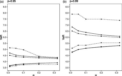
Figure 1 shows two-sided confidence limits of the VaR generated using the three different methods with security levels p = 0.95 (left) and p = 0.99 (right) for $1-\alpha \in \{0.68,0.8,0.9,0.95,0.99\}.$ The three methods included are BCA-VaR (determined using the computational tools), nonparametric, and parametric (using the computational tools). The values on the x-axis represent the wide range of α values considered to determine the $(1-\alpha )$-confidence intervals, and the values on the y-axis represent the bounds of the confidence intervals for the VaR. Several observations are drawn based on this data visualization. First, as expected based on results previously reported in the literature, the width of the confidence interval for VaR increases with a higher security level as well as smaller α values or higher coverage levels (see Miljkovic, Causey, and Jovanović 2022). Second, there are some new observations: The nonparametric confidence intervals are particularly different when the security level is 0.99: we see a strong increase in the upper bound of the confidence interval. The same phenomenon is observed for p = 0.95 when the coverage levels are above 0.8 ($\alpha <.2$). The lower bounds of the confidence intervals obtained with BCA-VaR and par-comp are visually the same for both security levels. The upper bounds of the confidence intervals for the BCA-VaR and par-comp differ slightly, with the BCA-VaR results providing higher upper bounds than those obtained with the par-comp method for both security levels and the discrepancy increasing with decreasing α values.

Figure 1. Two-Sided Confidence Limits for VaR for Security Level: (a) p = 0.95 and (b) p = 0.99. Note: Different line styles indicate the method used: BCA-VaR (solid line), par-comp (long dashed line), and non-par (dot-dashed line).

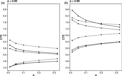
Similarly, we present the results for CTE in Figure 2. For p = 0.95, both BCA-CTE and par-comp generate the same results for the lower limit of the confidence intervals regardless of the confidence level implied by α. The results for the upper limits of both methods indicate that the BCA-CTE values are slightly above the par-comp values. The nonparametric confidence intervals for p = 0.95 are quite different from those obtained with the other two methods, in particular, the upper limits are considerably larger. Also, the lower limits for the nonparametric confidence intervals are above the lower limits of the other two methods except for very small values of α. For p = 0.99 the results for BCA-CTE and par-comp again rather closely align for the lower limits whereas the nonparametric estimates are much higher. The results are different for the upper limits where BCA-CTE leads to the highest upper limits for small α values followed by the nonparametric estimates, while for higher α values again the nonparametric approach results in the highest upper limits.

Figure 2. Two-Sided Confidence Limits for CTE for Security Level: (a) p = 0.95 and (b) p = 0.99. Note: Different line styles indicate the method used: BCA-CTE (solid line), par-comp (long dashed line), and non-par (dot-dashed line).

Complementing Figures 1 and 2, Table 1 provides the numerical summary of the confidence intervals for VaR and CTE for the Secura Re dataset when the left-truncated Lognormal model is fitted. Two security levels and three estimation methods are considered. The lower and upper bounds of the 95% ($\alpha =.05$) and 99% ($\alpha =.01$) confidence intervals are included for each estimation method.

Table 1 Summary of the Interval Estimates for VaR and CTE Based on the Secura Re Dataset

Method	$1-\alpha$	VaR	CTE
p = 0.95
non-par	0.95	(3.660, 5.093)	(4.597, 6.173)
par-comp	0.95	(3.745, 4.407)	(4.529, 5.608)
BCA	0.95	(3.759, 4.528)	(4.550, 5.759)
non-par	0.99	(3.586, 5.127)	(4.349, 6.420)
par-comp	0.99	(3.642, 4.510)	(4.360, 5.777)
BCA	0.99	(3.674, 4.703)	(4.366, 6.046)
p = 0.99
non-par	0.95	(5.343, 7.899)	(6.612, 7.942)
par-comp	0.95	(4.992, 6.308)	(5.804, 7.688)
BCA	0.95	(4.988, 6.525)	(5.903, 8.296)
non-par	0.99	(5.100, 7.899)	(6.403, 8.151)
par-comp	0.99	(4.785, 6.514)	(5.508, 7.984)
BCA	0.99	(4.766, 6.840)	(5.654, 8.742)

Table 2 provides the summary of the computational parametric and BCA estimates associated with the computation of the confidence intervals for VaR and CTE at two different security levels (0.95 and 0.99). The standard deviation of the distribution developed for the par-comp method is provided in the column labeled by ${\widehat{\sigma }}_{\text{par}}.$ The estimates of the standard deviation of the bootstrap distribution $G(·),$ defined by Equation (2.2)(2.2) $$\widehat{\theta }(\alpha )=G^{-1}\left\{\Phi \left[{\widehat{z}}_0+\frac{{\widehat{z}}_0+z_{\alpha }}{1-\widehat{a}({\widehat{z}}_0+z_{\alpha })}\right]\right\},$$(2.2) , are provided in the column labeled by ${\widehat{\sigma }}_{\text{boot}}.$ The values of the standard deviations are similar, with consistently slightly higher values for the BCA approach with the security level fixed. The skewness estimate of $G(·)$ is labeled as “Skew” and reported in the last column of the table. This indicates that $G(·)$ is slightly right-skewed. Bias correction and acceleration value estimates are reported in columns labeled as ${\widehat{z}}_0$ and $\widehat{a},$ respectively. These values are positive, indicating an upward correction to the standard confidence limits. According to Efron and Narasimhan 2020a (616), if $G(·)$ is right-skewed, the confidence limits should not be skewed to the left, at least for the distribution in the exponential family. The differences observed between the parametric and BCA methods in the estimation of the upper confidence limits for VaR and CTE raise doubts about the underlying statistical assumptions imposed for the par-comp approach being suitable, in particular given that the Secura Re dataset is only of moderate size with a skewness coefficient of 2.42. Rather, it is suggested that the results obtained from the BCA method provide better accuracy. In addition, we conjecture that the differences between the results of these two approaches may be even more pronounced for datasets exhibiting a stronger heavy tail such as those modeled by Miljkovic and Grün (2016).

Table 2 Summary of the Computational Parametric and BCA Estimates for VaR and CTE Based on the Secura Re Dataset

Measure	p	${\widehat{\sigma }}_{\mathit{par}}$	${\widehat{\sigma }}_{\mathit{boot}}$	${\widehat{z}}_0$	$\widehat{a}$	Skew
VaR	0.95	0.1687	0.1928	0.0790	0.0364	0.2518
	0.99	0.3356	0.3747	0.0301	0.0371	0.1622
CTE	0.95	0.2751	0.3205	0.0238	0.0372	0.2043
	0.99	0.4807	0.5627	0.0916	0.0363	0.2879

5. SIMULATION

In this section, we use a simulation study with artificial data where the true data generating process and hence the true values for VaR and CTE are known. Our objective is to compare the performance of the proposed BCA confidence intervals (BCA-VaR and BCA-CTE) with confidence intervals obtained using the nonparametric (non-par) as well as parametric (par-comp) approaches discussed in Section 3. The performance of these three methods is evaluated based on their coverage probability and the width of the confidence intervals calculated for different simulation settings. Coverage probability is estimated using the proportion of the confidence intervals that contain the true value of VaR or CTE. The width of the confidence interval is computed as the difference between the upper and lower bound estimates. We draw random samples from the left-truncated Lognormal distribution assuming that this distribution represents the true data generating process. Three sample sizes $n\in \{100,500,1000\}$ with two security levels $p\in \{0.95,0.99\}$ and confidence coefficients $1-\alpha \in \{0.68,0.8,0.9,0.95,0.99\}$ are considered.

The goal of the simulation study is to answer the following questions related to the BCA, nonparametric, and parametric methods used in construction of the confidence intervals:

1. How do the methods compare in terms of coverage probability also taking into account the width of the confidence interval?

2. How do the results of the BCA and the parametric approach differ for the left-truncated Lognormal model depending on the implementation; that is, if the general computational tools or the analytical solutions from Lemmas 1–5 are used for implementation?

The left-truncated Lognormal model was fitted to the Secura Re dataset used in Section 4 and parameter estimates were obtained using ML estimation. This model, together with the estimated parameters, was used as data generating processes in the simulation study. The datasets created in this way hence followed a distribution that mimics the data distribution observed for the Secura Re dataset. We generated 10,000 samples for each simulation setting. For calculation of the BCA confidence interval, each sample was bootstrapped 2000 times (i.e., resampled with B = 2000).

Figure 3 displays the multipanel plot of the simulation results related to the coverage probability and Figure 4 displays the multipanel plot of the simulation results related to the interval width. Each multipanel plot is arranged across several dimensions of the simulation study: we consider two risk measures, two security levels, and three sample sizes. For each of these 12 slices of data, we show how the coverage probability or interval width (y-axis) varies with the confidence coefficient (x-axis) across the three different estimation methods displayed with different line styles. The simulation results for the BCA method are shown with the black solid line and the non-par and par-comp methods are denoted by dotted and dashed lines, respectively.

Figure 3. Coverage Probability for the Left-Truncated Lognormal Distribution of the Three Estimation Methods: BCA (solid), non-par (dotted), par-comp (dashed). Note: Dashed gray lines denote the expected coverage probability.

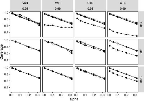
Figure 4. Average Width of the Confidence Interval for the Left-Truncated Lognormal Distribution of the Three Estimation Methods: BCA (solid), non-par (dotted), par-comp (dashed).

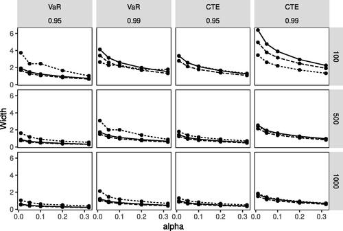
The VaR results (shown in the two left columns in Figures 3 and 4) indicate that the par-comp as well as the BCA approach provide comparable good coverage and similar width of the confidence intervals. The results of the nonparametric approach indicate that coverage is only reasonable if either the sample size is not too small or the security level is not too high (with the coverage results being poor for p = 0.99 and n = 100 in case of the nonparametric approach) and that the interval width in general is higher than for the other two approaches, except in the case where coverage was not satisfactory.

The CTE results (shown in the two right columns in Figures 3 and 4) indicate that coverage is again comparable good for the par-comp and the BCA approaches regardless of security level and sample size. Only considering the interval width the par-comp approach leads to considerably shorter intervals for p = 0.99 and n = 100. The non-par method proves inferior in terms of coverage and the interval width when p = 0.99 across all three sample sizes, with the coverage performance also being poor for the small sample size, n = 100 when p = 0.95.

The results of the simulation study were obtained for a setting where the true data generating process is a truncated Lognormal distribution that is also used as the parametric model in the parametric and BCA approaches for determining the confidence intervals. In this case, the results obtained with the nonparametric approach are clearly inferior for sample sizes up to 1000. In the case of the VaR, the nonparametric approach at least provides reasonable coverage in case $n\ge 500.$ But in all cases, the width of the confidence intervals is higher than for the other two approaches when coverage is satisfactory. The underlying assumptions of the parametric approach on the data generating process are met in this simulation study, and relying on the approximation based on the asymptotic normality seems to be reasonable. The BCA approach requires fewer assumptions and provides similar results and hence might be preferable in practice where the underlying data generating process is unknown.

To address the second question of the simulation study, we compare the results of the BCA approach as well as the parametric asymptotic approach depending on two different implementation methods: fully computational (method 1) and partially computational (method 2). Maximum likelihood estimation of the parameters given a dataset requires computational tools for both approaches regardless of the implementation. We also compare the coverage of method 1 and method 2 to their respective true coverages.

In the case of the BCA approach, the point estimates of the risk measures were found for the fully computational method using a root-finding algorithm (for VaR) and the numerical integration tools (for CTE) in R. When a partially computational method was used for the BCA approach, the point estimators of the risk measures were implemented using the analytical results obtained by Lemmas 1 and 2. The relative differences between method 1 and method 2 in percent were calculated for the width and coverage of the confidence intervals of both risk measures across all simulation settings. The ranges of these results are summarized in the top portion of Table 3. The columns labeled Δ_width and Δ_cov show the ranges of relative differences in percent between the two implementation methods. We observed minor differences between method 1 and method 2, indicating that these two methods are similar in terms of their performance and either one can be used in practice. The range of relative differences between coverage calculated by method 1 and the true coverage in percent is shown in the column labeled ${\Delta }_{\text{cov},1}.$ Similarly, the range of relative differences between coverage calculated by method 2 and the true coverage in percent is shown in the column labeled ${\Delta }_{\text{cov},2}.$ Both ${\Delta }_{\text{cov},1}$ and ${\Delta }_{\text{cov},2}$ results include zero within the given range, indicating that the calculated confidence intervals lead to over- as well as undercoverage compared to the true coverage.

Table 3 Comparison of the Implementation Methods (%): BCA (Top) and Parametric Asymptotic (Bottom).

Measure	Δwidth	Δcov	${\Delta }_{\text{cov},1}$	${\Delta }_{\text{cov},2}$
BCA approach
VaR	(–0.08, 0.15)	(–0.37, 0.25)	(–4.26, 0.08)	(–4.18, 0.18)
CTE	(–0.63, 0.05 )	(–0.44, 0.34)	(–4.29, 0.34)	(–4.51, 0.23)
Parametric asymptotic approach
VaR	(–8.44, –5.34)	(–6.29, –0.51)	(–6.29, –0.58)	(–3.09, 0.50)
CTE	(–9.27, –6.89)	(–7.00, –0.84)	(–6.66, –1.06)	(–3.51, 0.89)

Note: Δ_width denotes the range of relative differences in percent between method 1 and method 2 for the width of the confidence intervals. Δ_cov denotes the range of relative differences in percent between method 1 and method 2 for the coverage of the confidence intervals. ${\Delta }_{\text{cov},1}$ denotes the range of relative differences in percent between method 1 and the true coverage of the confidence intervals. ${\Delta }_{\text{cov},2}$ denotes the range of relative differences in percent between method 2 and the true coverage of the confidence intervals.

Similarly, the implementations of the parametric asymptotic confidence intervals were compared when using either the analytical solutions (method 1) provided by Lemmas 1–5 or using general computational tools (method 2) available in R for finding the Hessian of the log-likelihood function and the gradients of the variance function numerically. The results are summarized in the bottom portion of Table 3. The columns labeled Δ_width and Δ_cov show the ranges of the relative differences in percent between the two implementation methods. Here, the results point to some systematic differences in both width and coverage between the two methods. We again investigate which of the two methods has better coverage compared to the true coverage. Similar to the BCA implementation approach, we compute the range of relative differences between coverage calculated by method 1 and the true coverage in percent as shown in the column labeled ${\Delta }_{\text{cov},1}.$ The range of relative differences between coverage calculated by method 2 and the true coverage in percent is shown in the column labeled ${\Delta }_{\text{cov},2}.$ Based on these results, we note that method 1 implemented based on the analytical solutions of Lemmas 1–5 consistently underestimates the true coverage probability for both risk measures as observed in ${\Delta }_{\text{cov},1}.$ By contrast, the results for ${\Delta }_{\text{cov},2}$ include zero within the given range. Overall method 2, based on general computational tools, produces better coverage of the confidence intervals for both risk measures and should be adopted in practice.

Through this simulation study, we learned that the BCA approach can be used to validate the results of using the parametric asymptotic approach to determine the confidence intervals. For large sample sizes, both methods yield similar results. For small to moderate sample sizes, small differences between the two methods are observed when modeling the real dataset of Secura Re losses. In summary, the simulation study provided insightful information about the behavior of the three types of confidence intervals under consideration as well as the influence of the implementation used.

6. CONCLUSION

In this article, we advanced the study of interval estimation of risk measures in the actuarial literature. We proposed the automated bias-corrected and accelerated bootstrap confidence intervals, named BCA-VAR and BCA-CTE for VaR and CTE, respectively, using, in particular, the left-truncated Lognormal distribution. The performance of the proposed intervals was assessed in comparison to nonparametric and parametric asymptotic approaches based on the same parametric distribution. For the application of the parametric approach, we also obtained new analytical results required when using the Delta method and asymptotic theory to derive the confidence intervals, which were previously not available in the literature for the left-truncated Lognormal loss model.

Our results showed that the nonparametric approach to interval estimation is generally inferior to the other two methods. The asymptotic parametric approach relies on the asymptotic normality of the risk measure estimates as the sample size increases and the regulatory conditions are met. However, when this assumption is violated, the BCA method will provide a more realistic assessment of the uncertainty of the risk measure estimates.

When testing these three methods on the real Secura Re dataset, we found that the BCA and parametric approaches, generated similar results for the lower limit but slightly different results for the upper limit of the confidence interval. When the results of the parametric and the BCA methods agree, the results can be taken to be accurate and meaningful. But if these methods yield different results such as those observed for the upper limit, researchers should ask themselves whether the statistical assumptions of the parametric approach are likely to be violated, hence supporting the validity of the BCA method.

In future applications involving computations of the confidence intervals for risk measures, we recommend using the BCA method to validate the parametric results. If the two methods produce different results, the insurer should refer to the BCA method because its bias correction and acceleration procedures allow for a higher level of accuracy in the results.

We focused on the left-truncated Lognormal model to derive the empirical results and also provided analytical formulas for this parametric model. However, the computational tools outlined are rather generic and might easily be used for other nonparametric estimators where standard error estimates are available and any kind of parametric model regardless of the estimation method used; for example, using the method of trimmed moments instead of ML. The comparison of the empirical results obtained with the computational and analytical implementations confirms the reliability of the computational tools. Hence, our study can be easily extended to include other parametric models such as the composite models considered by Grün and Miljkovic (2019) with the efficient implementation of computational tools. The BCA approach would require that the user provides the loss data as well as the input functions $t_1()$ and $t_2()$ based on the considered parametric model to estimate the risk measures. For many composite models, these functions can be derived analytically. The BCA method can also be explored with the model averaging approach considered by Miljkovic and Grün (2021) to account for model uncertainty in the estimation of the confidence intervals.

Acknowlegements

We thank the editors and the anonymous reviewers for their helpful comments that improved the readability and quality of this article.

APPENDIX A.

Proof of Lemma 1

The cdf $F_b()$ of the observations in the truncated sample ${\mathit{x}}_b$ can be expressed using the corresponding untruncated cdf $F()$ as follows:

$$F_b(x)=P(X\le x|X>b)=\frac{P((X\le x)\cap (X>b))}{P(X>b)}=\frac{F(x)-F(b)}{1-F(b)}\mathit{1}(x>b),$$ where $\mathit{1}()$ is the indicator function. The inverse function $F_b^{-1}(p)=\inf \{x:F_b(x)\ge p\}$ provides the 100pth percentile of the left-truncated distribution of X, which gives the result for π_p.

APPENDIX B.

PROOF OF LEMMA 2

The estimator of CTE for the security level p (see Klugman, Panjer, and Willmot 2012) is defined as (B.1) $${\eta }_p=E(X|X>{\pi }_p)=\frac{1}{1-p}{\int }_{{\pi }_p}^{\infty }x{f}_b(x)dx,$$(B.1)

where $f_b(x)=\frac{\partial F_b(x)}{\partial x}.$ Consider the substitution $t=F_b(x).$ Then Equation (B.1) can be written in terms of the quantile function $F_b^{-1}(p)$ for $p\in (0,1).$ That is, (B.2) $${\eta }_p=\frac{1}{1-p}{\int }_p^1{F}_b^{-1}(t)dt.$$(B.2)

The quantile function for the left-truncated Lognormal distribution is given by $$F_b^{-1}(p)=e^{\mu +\sigma {\Phi }^{-1}[p+(1-p)\Phi (\frac{\hspace{0.17em}\log \hspace{0.17em}(b)-\mu }{\sigma })]}$$

and when this result is included directly in Equation (B.2), we obtain the following integral: $${\eta }_p=\frac{1}{1-p}{\int }_p^1{e}^{\mu +\sigma {\Phi }^{-1}[t+(1-t)\Phi (\frac{\hspace{0.17em}\log \hspace{0.17em}(b)-\mu }{\sigma })]}dt.$$

Using substitution $\vartheta ={\Phi }^{-1}[t+(1-t)\Phi (\frac{\hspace{0.17em}\log \hspace{0.17em}(b)-\mu }{\sigma })],$ the integral above simplifies to $${\eta }_p=\frac{e^{\mu }}{(1-p)[1-\Phi (\frac{\hspace{0.17em}\log \hspace{0.17em}(b)-\mu }{\sigma })]}{\int }_A^{\infty }{e}^{\sigma \vartheta }\phi (\vartheta )d\vartheta ,$$

where the lower limit of integration is set by $A={\Phi }^{-1}[p+(1-p)\Phi (\frac{\hspace{0.17em}\log \hspace{0.17em}(b)-\mu }{\sigma })]$ and the density of the standard normal distribution is $\phi (\vartheta )=\frac{1}{\sqrt{2}\pi }{e}^{-\frac{{\vartheta }^2}{2}}.$ By combining the exponents, the above integral becomes $${\eta }_p=\frac{e^{\mu }}{(1-p)[1-\Phi (\frac{\hspace{0.17em}\log \hspace{0.17em}(b)-\mu }{\sigma })]}{\int }_A^{\infty }\frac{1}{\sqrt{2\pi }}{e}^{\sigma \vartheta -\frac{1}{2}{\vartheta }^2}d\vartheta .$$

Rewrite the exponent as $\sigma \vartheta -\frac{1}{2}{\vartheta }^2=\frac{{\sigma }^2}{2}-\frac{{(\vartheta -\sigma )}^2}{2}$ and rearrange some terms. Consider the symmetry of the standard normal distribution, which implies $1-\Phi (\frac{\hspace{0.17em}\log \hspace{0.17em}(b)-\mu }{\sigma })=\Phi (\frac{\mu -\hspace{0.17em}\log \hspace{0.17em}(b)}{\sigma }).$ Then, with additional simple substitutions, we easily arrive at the final solution, $${\eta }_p=\frac{\hspace{0.17em}\exp \hspace{0.17em}(\mu +\frac{{\sigma }^2}{2})}{(1-p)\Phi \left(\frac{\mu -\hspace{0.17em}\log \hspace{0.17em}(b)}{\sigma }\right)}\Phi \left[\sigma -{\Phi }^{-1}\left(p+(1-p)\Phi \left(\frac{\hspace{0.17em}\log \hspace{0.17em}(b)-\mu }{\sigma }\right)\right)\right].$$

APPENDIX C.

PROOF OF LEMMA 3

Let $\mathit{H}=\left[\begin{array}{cc}{h}_{11}& h_{12}\\ h_{21}& h_{22}\end{array}\right]$ denote the Hessian matrix of the second-order partial derivatives h_ij for $i,j=1,2$ of the log-likelihood function under parameters μ and σ where $h_{11}=\frac{{\partial }^2\mathcal{l}(\mu ,\sigma )}{\partial {\mu }^2},$ $h_{12}=h_{21}=\frac{{\partial }^2\mathcal{l}(\mu ,\sigma )}{\partial \mu \partial \sigma },$ and $h_{22}=\frac{{\partial }^2\mathcal{l}(\mu ,\sigma )}{\partial {\sigma }^2}.$ The following simple equations $\frac{\partial \varphi (B)}{\partial \mu }=\frac{B}{\sigma }\varphi (B)$ and $\frac{\partial \varphi (B)}{\partial \sigma }=\frac{\varphi (B)B^2}{\sigma }$ as well as the application of the chain rule with some straightforward simplifications result in $$\begin{array}{l}\frac{{\partial }^2\mathcal{l}(\mu ,\sigma )}{\partial {\mu }^2}=-\frac{n}{{\sigma }^2}\frac{[B\varphi (B)[1-\Phi (B)]-{\varphi }^2(B)+{[1-\Phi (B)]}^2]}{{[1-\Phi (B)]}^2}\\ \frac{{\partial }^2\mathcal{l}(\mu ,\sigma )}{\partial {\sigma }^2}=-\frac{n}{{\sigma }^2}[\frac{(-2B\varphi (B)+B^3\varphi (B))[1-\Phi (B)]-B^2{\varphi }^2(B)}{{[1-\Phi (B)]}^2}+\\ 3\frac{\sum _{i=1}^n(\hspace{0.17em}\log \hspace{0.17em}(x_i)-\mu {)}^2}{n{\sigma }^2}-1]\\ \frac{{\partial }^2\mathcal{l}(\mu ,\sigma )}{\partial \mu \partial \sigma }=-\frac{n}{{\sigma }^2}\left[\frac{(B^2-1)\varphi (B)[1-\Phi (B)]-B{\varphi }^2(B)}{{[1-\Phi (B)]}^2}+\frac{2}{n}\frac{\sum _{i=1}^n(\hspace{0.17em}\log \hspace{0.17em}(x_i)-\mu )}{\sigma }\right].\end{array}$$

Using the standard formulas for the elements of the observed Fisher information, it follows that $$\{\begin{array}{c}{\mathcal{J}}_{11}=\frac{n}{{\sigma }^2}\frac{[B\varphi (B)[1-\Phi (B)]-{\varphi }^2(B)+{[1-\Phi (B)]}^2]}{{[1-\Phi (B)]}^2}\hfill \\ {\mathcal{J}}_{22}=\frac{n}{{\sigma }^2}\left[\frac{-2B\varphi (B)[1-\Phi (B)]-B^2\varphi (B)\Phi (B)}{{[1-\Phi (B)]}^2}+3\frac{\sum _{i=1}^n(\hspace{0.17em}\log \hspace{0.17em}(x_i)-\mu {)}^2}{n{\sigma }^2}-1\right]\hfill \\ {\mathcal{J}}_{12}={\mathcal{J}}_{21}=\frac{n}{{\sigma }^2}\left[\frac{(B^2-1)\varphi (B)[1-\Phi (B)]-B{\varphi }^2(B)}{{[1-\Phi (B)]}^2}+\frac{2}{n}\frac{\sum _{i=1}^n(\hspace{0.17em}\log \hspace{0.17em}(x_i)-\mu )}{\sigma }\right]\hfill \end{array}$$

as desired.

APPENDIX D.

PROOF OF LEMMA 4

The first derivatives of π_p with respect to the parameters μ and σ, respectively, are defined as $\frac{\partial {\pi }_p(\mu ,\sigma )}{\partial \mu }$ and $\frac{\partial {\pi }_p(\mu ,\sigma )}{\partial \sigma }.$ The derivative of the inverse cdf of the standard normal distribution for $0<p<1$ may be determined by $\frac{\partial {\Phi }^{-1}(p)}{\partial p}=\frac{1}{\varphi [{\Phi }^{-1}(p)]},$ which can be derived using any standard calculus book (i.e., Loomis and Sternberg 1968). Using this and the chain rule, we arrive at $$\begin{array}{l}\frac{\partial {\pi }_p(\mu ,\sigma )}{\partial \mu }={\pi }_p(\mu ,\sigma )\left(1+\frac{\sigma }{\varphi ({\Phi }^{-1}(p+(1-p)\Phi (B)))}(1-p)\varphi (B)\left(-\frac{1}{\sigma }\right)\right),\\ \frac{\partial {\pi }_p(\mu ,\sigma )}{\partial \sigma }={\pi }_p(\mu ,\sigma )({\Phi }^{-1}(p+(1-p)\Phi (B)))-\\ \mathrm{\hspace{1em}}\mathrm{\hspace{1em}}\frac{\sigma }{\varphi ({\Phi }^{-1}(p+(1-p)\Phi (B)))}(1-p)\varphi (B)\left(-\frac{B}{\sigma }\right)),\end{array}$$

where $B=\frac{\hspace{0.17em}\log \hspace{0.17em}(b)-\mu }{\sigma }.$

APPENDIX E.

PROOF OF LEMMA 5

The first derivatives of η_p with respect to the parameters μ and σ, respectively, are defined as $\frac{\partial {\eta }_p(\mu ,\sigma )}{\partial \mu }$ and $\frac{\partial {\eta }_p(\mu ,\sigma )}{\partial \sigma }.$ Using the chain rule and some straightforward simplifications, we arrive at $$\frac{\partial {\eta }_p(\mu ,\sigma )}{\partial \mu }=\frac{A}{(1-p)}\frac{1}{[1-\Phi (B)]}\left[\Phi (C)-\frac{\varphi (B)}{\sigma [1-\Phi (B)]}\Phi (C)+\frac{\partial \Phi (C)}{\partial \mu }\right]$$ $$\frac{\partial {\eta }_p(\mu ,\sigma )}{\partial \sigma }=\frac{A}{(1-p)}\frac{1}{[1-\Phi (B)]}\left[\Phi (C)\sigma -\frac{B\varphi (B)}{\sigma [1-\Phi (B)]}\Phi (C)+\frac{\partial \Phi (C)}{\partial \sigma }\right].$$

The partial derivatives of $\frac{\partial \Phi (C)}{\partial \mu }$ and $\frac{\partial \Phi (C)}{\partial \sigma }$ are determined separately. Using again $\frac{\partial {\Phi }^{-1}(p)}{\partial p}=\frac{1}{\varphi [{\Phi }^{-1}(p)]}$ and after applying the chain rule to a composite function and performing some simplifications, we obtain the desired solution in closed form as follows: $$\frac{\partial \Phi (C)}{\partial \mu }=\varphi (C)\frac{(1-p)\varphi (B)}{\sigma \varphi ({\Phi }^{-1}(p+(1-p)\Phi (B)))}$$ $$\frac{\partial \Phi (C)}{\partial \sigma }=\varphi (C)\left(1+\frac{(1-p)B\varphi (B)}{\sigma \varphi ({\Phi }^{-1}(p+(1-p)\Phi (B)))}\right).$$

References

- Beirlant, J., Y. Goegebeur, J. Segers, and J. L. Teugels. 2004. Statistics of extremes: Theory and applications. Chichester, West Sussex: John Wiley & Sons.
- Blostein, M., and T. Miljkovic. 2019. On modeling left-truncated loss data using mixtures of distributions. Insurance: Mathematics and Economics 85:35–46.
- Blostein, M., and T. Miljkovic. 2021. ltmix: Left-truncated mixtures of Gamma, Weibull, and Lognormal distributions. R package version 0.2.1. https://CRAN.R-project.org/package=ltmix
- Brazauskas, V., B. L. Jones, M. L. Puri, and R. Zitikis. 2008. Estimating conditional tail expectation with actuarial applications in view. Journal of Statistical Planning and Inference 138 (11):3590–604.
- Brazauskas, V., B. L. Jones, and R. Zitikis. 2009. Robust fitting of claim severity distributions and the method of trimmed moments. Journal of Statistical Planning and Inference 139 (6):2028–43.
- Brazauskas, V., and T. Kaiser. 2004. “Empirical estimation of risk measures and related quantities,” Bruce L. Jones and Ricărdas Zitikis, October 2003. North American Actuarial Journal 8 (3):114.
- DasGupta, A. 2008. Asymptotic theory of statistics and probability. Vol. 180. New York, NY: Springer.
- DiCiccio, T. J., and B. Efron. 1996. Bootstrap confidence intervals. Statistical Science 11 (3):189–228.
- Efron, B. 1979. Bootstrap methods: Another look at the jackknife. The Annals of Statistics 7 (1):1–26.
- Efron, B. 1987. Better bootstrap confidence intervals. Journal of the American Statistical Association 82 (397):171–85.
- Efron, B., and T. Hastie. 2016. Computer age statistical inference. Vol. 5. New York, NY: Cambridge University Press.
- Efron, B., and B. Narasimhan. 2020a. The automatic construction of bootstrap confidence intervals. Journal of Computational and Graphical Statistics 29 (3):608–19.
- Efron, B., and B. Narasimhan. 2020b. bcaboot: Bias corrected bootstrap confidence intervals. R package version 0.2-3. https://CRAN.R-project.org/package=bcaboot
- Gilbert, P., and R. Varadhan. 2019. numDeriv: Accurate numerical derivatives. R package version 2016.8-1.1. https://CRAN.R-project.org/package=numDeriv
- Gnedenko, B. V. 1950. Kurs teorii veroyatnostyey [Probability theory course]. Moscow: Gosudarstvennoye Izdatyel’stvo Technico-Teoreticheskoi Literaturi.
- Grün, B., and T. Miljkovic. 2019. Extending composite loss models using a general framework of advanced computational tools. Scandinavian Actuarial Journal 2019 (8):642–60.
- Hogg, R. V., J. McKean, and A. T. Craig. 2005. Introduction to mathematical statistics. Upper Saddle River, NJ: Pearson Education.
- Hosking, J. R., and J. R. Wallis. 1987. Parameter and quantile estimation for the generalized Pareto distribution. Technometrics 29 (3):339–49.
- Kaiser, T., and V. Brazauskas. 2006. Interval estimation of actuarial risk measures. North American Actuarial Journal 10 (4):249–68.
- Kelley, K. 2005. The effects of nonnormal distributions on confidence intervals around the standardized mean difference: Bootstrap and parametric confidence intervals. Educational and Psychological Measurement 65 (1):51–69.
- Kim, J. H. T., and M. R. Hardy. 2007. Quantifying and correcting the bias in estimated risk measures. ASTIN Bulletin 37 (2):365–86.
- Klugman, S. A., H. H. Panjer, and G. E. Willmot. 2012. Loss models: From data to decisions. 4th ed. Hoboken, NJ: John Wiley & Sons.
- Loomis, L. H., and S. Sternberg. 1968. Advanced calculus. Reading, Massachusetts: Addison-Wesley.
- Manistre, J. B., and G. H. Hancock. 2005. Variance of the CTE estimator. North American Actuarial Journal 9 (2):129–56.
- Micceri, T. 1989. The unicorn, the normal curve, and other improbable creatures. Psychological Bulletin 105 (1):156–66.
- Miljkovic, T., R. Causey, and M. Jovanović. 2022. Assessing the performance of confidence intervals for high quantiles of Burr XII and inverse Burr mixtures. Communications in Statistics – Simulation and Computation 51 (8):4677–99.
- Miljkovic, T., and B. Grün. 2016. Modeling loss data using mixtures of distributions. Insurance: Mathematics and Economics 70:387–96.
- Miljkovic, T., and B. Grün. 2021. Using model averaging to determine suitable risk measure estimates. North American Actuarial Journal 25 (4):562–79.
- Necir, A., A. Rassoul, and R. Zitikis. 2010. Estimating the conditional tail expectation in the case of heavy-tailed losses. Journal of Probability and Statistics 2010:1–17.
- Poudyal, C. 2021. Robust estimation of loss models for lognormal insurance payment severity data. ASTIN Bulletin 51 (2):475–507.
- R Core Team. 2021. R: A language and environment for statistical computing. Vienna, Austria: R Foundation for Statistical Computing. https://www.R-project.org/
- Reynkens, T., R. Verbelen, J. Beirlant, and K. Antonio. 2017. Modelling censored losses using splicing: A global fit strategy with mixed Erlang and extreme value distributions. Insurance: Mathematics and Economics 77:65–77.
- Serfling, R. 1980. Approximation theorems of mathematical statistics. New York: Wiley.
- Tibshirani, R. 1988. Variance stabilization and the bootstrap. Biometrika 75 (3):433–44.
- Tucker, H. G. 1959. A generalization of the Glivenko-Cantelli theorem. The Annals of Mathematical Statistics 30 (3):828–30.
- Verbelen, R., L. Gong, K. Antonio, A. Badescu, and S. Lin. 2015. Fitting mixtures of Erlangs to censored and truncated data using the EM algorithm. ASTIN Bulletin 45 (3):729–58.