Key Drivers of Long-Term Rates of Mortality Improvements in the United States: Period, Cohort, and Cause of Death Analysis, 1959–2016

Abstract

The main objective of this article is to identify significant mortality drivers in the U.S. population that have a high likelihood of being linked to the historical improvement or deterioration of mortality over the 1959 to 2016 period. To achieve this objective, we integrate cause of death modeling with epidemiological evidence to explain the underlying drivers. In particular, we analyze cause of death data for six broad groups of causes including circulatory diseases, neoplasms, respiratory diseases, digestive system diseases, external causes, and other causes. We also identify and analyze some key causes that serve as markers of trends in behavioral risk factors that could drive mortality change. These risk factors are AIDS and tuberculosis, alcohol abuse, dementia and Alzheimer’s disease, diabetes and obesity, drug dependency, homicide, hypertensive disease, self-harm, and smoking. We analyze these different groupings of causes of death using life expectancy decomposition techniques and formal age–period–cohort decomposition of both mortality rates and mortality improvement rates. We find that the story of mortality evolution in the United States in the second half of the 20th century, which continued into the first decade of the 21st century, has been mainly a story of mortality improvements from circulatory diseases. Nevertheless, despite the clear dominance of circulatory diseases as a leading cause of death and as the main contributor to mortality improvements between 1959 and 2016, the decline in mortality has been more complex. The trajectories of other major causes have ebbed and flowed, and the patterns of behavioral risk factors that contribute to overall mortality change have seen changes between generations.

1. INTRODUCTION

The understanding of the drivers behind mortality change is a topic that has attracted significant attention in the epidemiological, medical, and economic literature. The Society of Actuaries (SOA) has recognized this and has recently commissioned a series of studies to understand the different components behind mortality trends in the U.S. population and thus get a better understanding of possible future trends. This series of studies aims to move from looking only at all-cause mortality at the national U.S. level (Li, Zhou, and Liu 2017a,b Liu et al. 2020) to looking at the causes of death (Villegas et al. 2021) and subpopulation trends (Barbieri 2020, 2021) underpinning this total mortality. The goal of this article is to present a summary of the main results of one of these studies, in which we integrate cause of death modeling with epidemiological evidence to identify significant mortality drivers in the U.S. population that have a high likelihood of being linked to the historical improvement or deterioration of mortality over the 1959 to 2016 period (Villegas et al. 2021).

Recently, there have been important academic contributions to the understanding of mortality change in the United States Chief among these contributions was the widely publicized work of Case and Deaton (2015) reporting an increase in mortality rates among middle-aged U.S. white men and women with low levels of education. They argued that this was a cohort effect and that the reversal in the long-term decline in the all-cause mortality rate was largely driven by increases in deaths from suicides, alcohol and drug poisonings, and chronic liver diseases and cirrhosis (pooled for analysis as “deaths of despair”). Subsequently, Masters, Tilstra, and Simon (2018) applied age–period–cohort (APC) methods to analyze trends for each of these causes separately for men and women and confirmed that deaths for middle-aged whites had increased in the 21st century but primarily because of rapid increases in drug-related mortality from the late 1990s rather than in suicides or alcohol use and, crucially, that this increase was a period rather than a cohort effect linked to prescribed opioid use. In an earlier paper, Masters et al. (2014) employed an APC model to study the long-term trend in all-cause and cause-specific mortality for the U.S. black and white populations over the 1959 to 2009 period and found clear cohort-based trends in heart disease, stroke, lung cancer, female breast cancer, and other cancer mortality, accompanied by especially pronounced period-based reductions in mortality from heart disease, stroke, infectious diseases, and homicide.

Despite the long-term trend in health and mortality improvements in the United States, recent research has highlighted the persistence and widening of trends in inequalities in life expectancy by socioeconomic circumstances measured at either the individual level (e.g. educational attainment, relative income, race/ethnicity) or area level (unemployment, poverty, urban–rural) or analyzed for all causes or partitioned into major causes of death (Chetty et al. 2016; Singh et al. 2017; Masters, Tilstra, and Simon 2018). The pace of change has varied with the unit of analysis, the causes of death, and specific age groups; but essentially the overall pattern has been one of heterogeneity and unequal gains in mortality improvements.

Some of the newly emerging insights point to possible causal mechanisms driving the gradient in life expectancies. Chetty et al. (2016) found that at the county level, life expectancy in middle age for low-income people was highly correlated with health behaviors (e.g., smoking, obesity) but not significantly associated with area differences in levels of medical care. Like in England (Marmot 2010), they also found that life expectancy of low-income men varied more between geographic areas than it did for more advantaged men, implying that unmeasured contextual factors play a role in addition to compositional factors in the spatial patterns of disadvantage at an area level (Macintyre, Ellaway, and Cummins 2002). They also found little association between life expectancy variation and health care access variables.

Our article aims to bring clarity and structure to this mortality change debate by using decomposition methods borrowed from demography and formal APC modeling to analyze a carefully considered selection of causes of death. A starting point for a structured analysis of mortality trends is to establish a grouping of causes that can be linked to possible drivers of mortality change over the last 6 decades. One comprehensive, four-level hierarchical grouping of causes is the Global Burden of Disease (GBD), which allows the ranking of causes of death at varying levels of detail (Wang et al. 2016). For example, Dwyer-Lindgren et al. (2016) studied deaths in the United States from 1980 to 2014 at Level 2 of the GBD groupings (with 21 groups). In 2014, the leading three causes of death were circulatory diseases, neoplasms, and neurological disorders. In addition, Dwyer-Lindgren et al. (2016) found that whereas some major causes of death such as circulatory diseases and neoplasms recorded a reduction in mortality rates between 1980 and 2014, other causes such as neurological diseases and mental and substance abuse disorders showed the opposite trend with a significant increase in mortality rates.

In another study, Mokdad et al. (2018) applied the GBD methodology to analyze health trends in the United States between 1990 and 2016. At the more detailed Level 3 grouping of the GBD, they reported that ischemic heart disease (IHD) remained the leading cause of death in 2016 despite a reduction of 50.7% in its age-standardized death rate (ASDR) between 1990 and 2016. The next four leading causes of death in 2016 were cancer of the trachea, bronchus, and lung; chronic obstructive pulmonary disease; Alzheimer’s disease and other dementias; and cancer of the colon and rectum. Notably, Alzheimer’s disease and other dementias were only the seventh leading cause of death in 1990 but climbed to the fourth position in 2016 because of an increase of 11.3% in their ASDR. By contrast, deaths due to motor vehicle road injuries passed from being ranked the third cause of death in 1990 to the sixth cause in 2016 as result of a decline of 35.4% in its ASDR.

A step beyond the analysis of mortality trends by causes of death group is the identification of the main risk factors associated with mortality. For example, McGinnis and Foege (1993) introduced the concept of actual causes of death to identify and quantify the major external factors that contribute to death. Applying this concept, Mokdad et al. (2004) reported that in 2000 the top three leading causes of death in the United States were tobacco, poor diet and physical inactivity, and alcohol consumption. Other factors identified by Mokdad et al. (2004) included microbial agents, toxic agents, motor vehicle crashes, incidents involving firearms, sexual behaviors, and illicit use of drugs.

The GBD has also developed a comprehensive approach for the evaluation of risk factors, their association with causes of death, and their contribution to total deaths (GBD 2017 Risk Factor Collaborators 2018). The GBD approach uses medical studies to quantify the relationship between 84 risk factors and multiple causes of death. By amalgamating the causes of death across the different risk factors, it is then possible to map each risk factor to the number of deaths attributable to it. These risk factors are grouped into three broad categories to aid interpretation, namely, behavioural, environmental and occupational, and metabolic risks. Using the GBD framework, Mokdad et al. (2018) identified that in 2016 the top seven risk factors associated with U.S. mortality belonged to the behavioral and metabolic categories. The leading behavioral risk factors were dietary risks, tobacco, and alcohol and drug use, and the top metabolic factors were hypertension, obesity, diabetes, and high cholesterol.

In this article we adopt an indirect approach to measuring the effect of these known drivers of mortality change. To proxy the impact of behavioral risk factors and access to health care on mortality change, we propose to use mortality partitioning by cause of death into biologically relevant subcomponents. For example, Carnes et al. (2006) partitioned deaths into intrinsic and extrinsic components. Of those classed as extrinsic (i.e., related to exogenous environmental factors), others have further partitioned deaths into specific markers of risky behaviours; for example, smoking-related deaths, deaths related to alcohol and drug misuse, deaths related to obesity (Dwyer-Lindgren et al. 2016; Masters, Tilstra, and Simon 2018), and deaths related to causes amenable to health care treatment (Nolte and McKee 2012).

After deriving a suitable classification of mortality according to causes of death, we use two main approaches for understanding trends in mortality change. First, to obtain an assessment of the age groups and causes of death driving the temporal improvement in life expectancy, we apply life expectancy decomposition methods borrowed from demography such as the Arriaga method (Arriaga 1984). Such methods have the advantage of enabling a simple and easy-to-communicate graphical representation of the contribution of each age group and cause of death to gains in life expectancy over a certain period of time.

Second, we use APC modeling to identify and understand the driving forces behind mortality change. On the one hand, age is perhaps the clearest marker of mortality patterns, with certain causes of death being more prominent at different ages. On the other hand, trends in mortality are the result of changes in environmental and social factors that may manifest themselves as period or cohort effects. In particular, to disentangle the period and cohort components of mortality change, this article relies on the period–cohort improvement (PCi) rate model: $$-\hspace{0.17em}\mathrm{\text{log}}\hspace{0.17em}\frac{m_{x,t}}{m_{x,t-1}}=\alpha +{\tilde{\kappa }}_t+{\tilde{\gamma }}_{t-x},$$ where $m_{x,t}$ is the mortality rate at age $x$ in year $t$ and $-\hspace{0.17em}\mathrm{\text{log}}\hspace{0.17em}\frac{m_{x,t}}{m_{x,t-1}}$ are the corresponding mortality improvement rates. This model decomposes the mortality improvements into the average mortality improvements for all ages during the 1959 to 2016 study period captured by $\alpha ,$ the period (calendar year) deviations from these average improvements captured by $\widetilde{{\kappa }_t},$ and the cohort (year of birth) deviations from these average improvements captured by ${\tilde{\gamma }}_{t-x}.$ As we will discuss in Section 4.1, the PCi model is the equivalent of the standard APC mortality rate model that has previously been considered in the decomposition of cause-specific U.S. mortality trends into APC components (Yang 2008; Masters et al. 2014; Masters, Tilstra, and Simon 2018).

The rest of this article is organized as follows. In Section 2 we describe our main data sources and set out the rationale for the choice of cause of death groupings for use in our analysis. In Section 3 we discuss the life expectancy decomposition methodology we use to identify the causes of death that contribute the most to life expectancy change. In Section 4 we focus on the systematic decomposition of cause-specific mortality trends across the dimensions of age, period, and cohort using well-known actuarial and demographic modeling techniques. In Section 5 we integrate epidemiological evidence with the application of the life expectancy decomposition methods and the PCi model to identify key drivers behind period and cohort trends in mortality change in the United States between 1959 and 2016. Finally, Section 6 provides some concluding comments and identifies areas for further research.

2. DATA

We use a bespoke cause of death dataset based on data stemming from the Human Cause of Death Database (2020) and the Human Mortality Database Cause of Death Data (HMD COD). The HMD COD is an SOA-sponsored initiative to develop a cause of death extension of the Human Mortality Database (2020). These data, which are described in Barbieri (2017), provide age-specific mortality rates for 92 subcategories of death.

Our dataset consists of cause of death mortality data by single year of age for the period 1959 to 2016. Over this period, cause of death coding followed four different International Classification of Diseases (ICD) regimes as summarized in Table 1. For the period 1959 to 1978, our data come from the HMD COD dataset and are not adjusted for ICD coding changes between ICD-7 and -8. This is joined with a preliminary version of the Human Cause of Death Database for the period 1979 to 2016 that uses bridge coding to adjust for ICD coding changes between ICD-9 and -10. There are no adjustments made for the discontinuity between ICD-8 and -9.

TABLE 1 Years of ICD Regimes

Regime	ICD-7	ICD-8	ICD-9	ICD-10
Years	1959–1967	1968–1978	1979–1998	1999–2016

For the purposes of our analysis, we use a mapping from the ICD three- or four-digit code to the 92 subcategories of death proposed by the authors of the HMD COD. The approach they took was to identify groups of clinically related codes that were broadly equivalent in terms of medical content across the ICD coding regimes. This somewhat ameliorates the problem of major discontinuities due to ICD regime changes. We initially group all deaths by these 92 subcategories, which we will refer to as the 92 causes. The details of this grouping with the three digit codes composing each of the 92 subcategories are described in Barbieri (2017, appendix A).

2.1. Causes of Death Grouping for Analysis

We have carefully considered the groupings of causes that we wish to analyze. If the number of groupings chosen is too large, any broad trends or patterns in mortality will be difficult to determine. In contrast, if the number of groupings is too small, the information will not be as useful because any heterogeneity in trends within groupings of causes is masked.

Accordingly, for our analysis we have developed a further aggregation of the 92 causes of death under two levels: a first Level 1 grouping comprising six broad groups and a Level 2 more detailed grouping with some of the main subcauses within each Level 1 cause. This two-level grouping of causes is summarized in Table 2, where we indicate the mapping of each of our grouping of causes to the 92 causes used by the HMD COD.

TABLE 2 Cause of Death Groupings and Age–Standardized Death Rate for Selected Years

Level 1	Level 2	HMD cause groups	ASDR female			ASDR male
			1959	2016	%Change	1959	2016	%Change
All-cause			1353.03	757.73	–44.00	1507.75	788.94	–47.67
Circulatory diseases			867.84	230.53	–73.44	882.93	237.47	–73.10
	Ischemic heart disease	47	377.57	85.48	–77.36	499.56	116.42	–76.70
	CVD and stroke	51	220.58	46.59	–78.88	169.38	32.86	–80.60
	Other circulatory system diseases	45, 46, 48, 49, 50, 52, 53, 54, 55	269.69	98.46	–63.49	213.99	88.19	–58.79
Neoplasms			199.40	163.95	–17.77	222.60	180.04	–19.12
	Bowel cancer	13, 14	34.33	14.30	–58.34	30.64	15.76	–48.54
	Liver cancer	15	9.56	6.23	–34.84	7.45	10.90	46.28
	Lung cancer	18	7.72	38.03	392.79	44.02	44.80	1.77
	Breast cancer	20	35.98	23.60	–34.42	0.35	0.26	–25.59
	Prostate cancer	24				25.48	16.55	–35.05
	Other cancers	17, 19, 21, 22, 23, 25, 26, 27, 28, 29, 30, 31, 32	84.40	64.02	–24.14	67.11	64.77	–3.49
	Other digestive organ cancers	10, 11, 12, 16	27.42	17.78	–35.16	47.57	27.00	–43.23
Respiratory diseases			61.13	76.58	25.27	83.52	71.30	–14.63
	Influenza and pneumonia	56, 58	48.00	14.86	–69.03	51.21	13.75	–73.15
	Chronic lower respiratory disease	59, 60, 61	7.52	45.81	509.23	22.34	40.13	79.61
	Other respiratory diseases	57, 62	5.61	15.91	183.31	9.96	17.43	74.89
Digestive system			40.17	28.27	–29.63	55.13	32.27	–41.46
	Gastric and duodenal ulcer	63	4.97	0.88	–82.27	12.99	0.93	–92.87
	Chronic liver disease	65	9.42	8.54	–9.33	18.50	15.23	–17.69
	Other digestive system diseases	64, 66	25.78	18.84	–26.91	23.64	16.12	–31.80
External causes			56.33	44.75	–20.55	114.11	98.00	–14.12
	Traffic accidents	84	12.05	3.93	–67.40	36.34	10.75	–70.42
	Self–harm and interpersonal violence	89, 90	7.98	8.58	7.53	28.32	31.04	9.61
	Other external causes	85, 86, 87, 88, 91, 92	36.30	32.24	–11.18	49.46	56.21	13.66
Other			128.17	213.65	66.70	149.46	169.85	13.65
	AIDS and tuberculosis	1, 8	4.65	1.10	–76.41	12.39	3.00	–75.76
	Diabetes and obesity	34, 35	28.58	22.63	–20.81	18.57	27.03	45.58
	Alcohol abuse and drug dependence	37, 38	0.67	2.04	206.68	3.08	5.82	88.95
	Alzheimer’s disease	42		45.08			18.99
	Dementia and other mental disorders	39	1.63	44.12	2603.21	1.12	21.29	1800.06
	Rest of causes	2, 3, 4, 5, 6, 7, 9, 33, 36, 40, 41, 43, 44, 67, 68, 69, 70, 71, 72, 73, 74, 75, 76, 77, 78, 79, 80, 81, 82, 83	92.64	98.68	6.52	114.30	93.72	–18.01

The Level 1 grouping allows us to get an initial overview of cause-specific trends. The Level 2 grouping decomposes the Level 1 causes into leading causes of death, allowing us to drill down on the trends observed at Level 1 by looking at trends for individual causes that merit a separate analysis and interpretation. For instance, separate trends in ischemic heart disease and cardiovascular disease (CVD) and stroke are easier to interpret than trends from the broader circulatory disease group.

To gauge the overall magnitude of the different causes of death, in Table 2 we report the ASDR by Level 1 and Level 2 causes in years 1959 and 2016. To compute the ASDR, we use the U.S. gender-specific 2010 census population as our standard (National Bureau of Economic Research 2016), along with cause-specific mortality rates for ages 0, 1–4, 5–9, …, 100+. Specifically, the ASDR is calculated as $$\mathit{\text{ASDR}}=\frac{\sum _x{m}_x{E}_x}{\sum _x{E}_x}\times 100,000,$$ where x is each age band (e.g., 0, 1–4, 5–9,…, 100+), m_x is the mortality rate for that age band, and E_x is the reference population for that age band. For ease of reading, we report the ASDRs as rates per 100,000 of standard population.¹ We also report in Table 2 the percentage change in ASDR between 1959 and 2016.

In Table 2 we see that the all-cause ASDR fell by almost a half between 1959 and 2016, from 1508 to 789 (per 100,000) for men and from 1353 to 758 for women. This decrease was accompanied by an important change in the cause of death composition. Whereas in 1959 circulatory diseases accounted for 59% and 64% of the all-cause ASDR for males and females, respectively, in 2016 circulatory diseases accounted for only 30% for both genders. As a result, neoplasms are starting to replace circulatory disease as the leading cause of death. For both genders, neoplasms accounted for just 15% of the all-cause ASDR in 1959, increasing to about 23% in 2016. The “other” group of Level 1 causes has also increased in importance. This group accounted for just about 10% of the all-cause ASDR in 1959 for both genders, doubling to 22% in 2016 for males and tripling to 28% in 2016 for females.

2.2. Risk Factors and Drivers of Mortality Change

We also consider some key causes that can serve as markers of trends in behavioral risk factors that could drive mortality change. We identified nine factors that we have mapped to causes of death according to Table 3. This “risk factor” grouping of causes of death facilitates the recognition of behavioral trends that might be less noticeable when analyzing the individual causes at the Level 1 and Level 2 groupings.

TABLE 3 Risk Factors and Drivers of Mortality Change Groupings

Risk factor	Associated cause of death	HMD Cause groups	ASDR female			ASDR male
			1959	2016	%Change	1959	2016	%Change
AIDS and tuberculosis	AIDS and tuberculosis	1, 8	4.65	1.10	–76.41	12.39	3.00	–75.76
Alcohol abuse	Alcohol abuse and poisoning, chronic liver disease	37, 65, 86	10.11	10.16	0.49	21.86	20.69	–5.34
Dementia and Alzheimer’s disease	Dementia and Alzheimer’s disease	39, 42, 80	7.87	90.73	1052.71	4.29	40.96	855.79
Diabetes and obesity	Diabetes and obesity	34, 35	28.58	22.63	–20.81	18.57	27.03	45.58
Drug dependency	Drug dependency	38, 87	1.08	11.85	992.35	2.01	25.50	1165.68
Homicide	Homicide	90	2.44	2.37	–2.71	7.70	9.66	25.38
Hypertensive disease	Hypertensive disease	48	92.57	24.09	–73.98	65.02	22.25	–65.78
Self–harm	Self–harm	89	5.55	6.21	12.03	20.61	21.38	3.71
Smoking	Lung cancer	18	7.72	38.03	392.79	44.02	44.80	1.77

Some of the risk factor groupings in Table 3 have a direct mapping with the causes defined in our Level 2 grouping in Table 2. However, others combine or split some of the Level 2 groupings to align better with risk factors known to cause a large proportion of deaths for that cause. For example, for alcohol abuse, in additions to deaths from chronic liver diseases and cirrhosis (HMD cause group 65) and from accidental poisoning from alcohol (HMD cause group 86), we include the deaths under mental and behavioral disorders (HMD cause group 37). Similarly, for drug dependency we include the deaths both from mental and behavioral disorders (HMD cause group 38) and from other accidental poisoning (HMD cause group 87). We note that HMD group 87 also includes ICD-10 codes X46–X49 that are not related to drug abuse, but these are small relative to codes X40–44, which account for drug-related poisoning.

We combine Alzheimer’s disease and dementia because they are related causes and often coded interchangeably by the certifying doctor. In contrast, we consider self-harm and homicide separately because they tend to exhibit different trends across the period and cohort dimensions. Though smoking contributes to deaths from heart disease, respiratory diseases, and many cancers, we use lung cancer as the marker for tracking smoking behavior because about 80% or more of lung cancer deaths are attributable to smoking (Ezzati and Lopez 2003).

Figure 1 shows the ASDR trends for the causes of death associated with each risk factor. The corresponding ASDR values in 1959 and 2016 are shown in Table 3. These causes of death are only meant to act as proxies for the selected risk factors and will inevitably underestimate the mortality attributable to, or linked to, a particular risk factor. Thus, when analyzing risk factors, we focus on trends and temporal changes rather than on the absolute values of the ASDRs.

FIGURE 1. Age-Standardized Death Rate for Selected Risk Factors, 1959–2016.

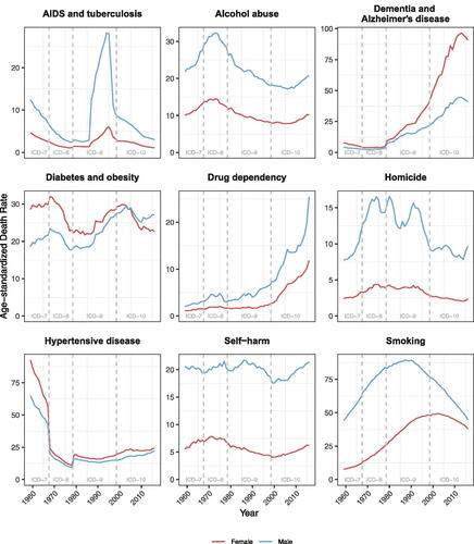
In brief, the main patterns we find in Figure 1 are as follows:

• AIDS and tuberculosis mortality rates show an important spike in the late 1980s and early 1990s with a significant and steady decrease from 2000 onwards.

• There has been an increase in mortality due to alcohol abuse, drug dependency, and self-harm since around early 2000s for both males and females. The trend for drug dependency is particularly noteworthy, because it can be seen from Table 3 that it has increased substantially from a very low base in 1959.

• Mortality rates due to dementia and Alzheimer’s disease have seen a significant increase since the 1980s, albeit with a slight reversal in trend since around 2013.

• Mortality rates from diabetes and obesity are driven largely by diabetes. This increased in the 1980s for both male and females, continuing in the 1990s for males, though recently post-2010 it has declined or remained flat.

• Homicide rates are quite volatile and do not seem to exhibit a clear pattern for males; for females the pattern is broadly flat.

• After a significant decrease between 1960 and 1980, there has been an increase in hypertensive disease mortality rates since the 1990s for both males and females. It is noticeable that hypertensive disease together with diabetes and obesity are the only two risk factors for which women have a higher ASDR than men. It also worth noting that there is some impact of coding changes for hypertensive disease affecting mainly the ICD-8 period.

• Mortality rates due to smoking have declined since 1990s for males and since 2000 for females.

3. LIFE EXPECTANCY DECOMPOSTION METHODOLOGY

We use life expectancy decomposition methods borrowed from demography to identify the ages and causes of death contributing the most to the change in life expectancy over different periods. Such methods have the advantage of enabling a simple and easy-to-communicate graphical representation of the contribution of each age group and cause of death to gains in life expectancy over a certain period of time.

More specifically, we use the formulae given in Andreev, Shkolnikov, and Begun (2002) and Shkolnikov, Andreev, and Begun (2003) to decompose the change in period life expectancy at age 20 by 5-year age band, by 92 causes of death and single calendar year. We then aggregate this decomposition to appropriate age groups, group of causes, and time periods. The formulae we use for the life expectancy decomposition are given in the Appendix. We note that our life expectancy calculations start at age 20. This is to avoid the possible complications that infant and child mortality may bring to our analysis.

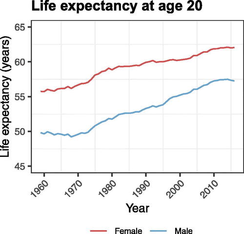
In Figure 2 we see that period life expectancy at age 20 in the United States increased significantly for both genders during the period 1959 to 2016, with the majority of this increase occurring post 1970. Life expectancy at age 20 moved from 55.75 years for females and 49.82 years for males in 1959 to 62.06 and 57.26 years in 2016, for an increase of 6.31 and 7.44 years for females and males, respectively.

FIGURE 2. Period Life Expectancy at Age 20, 1959–2016.

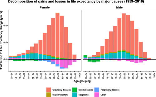
Figure 3 shows the contribution of different ages and causes to these changes in life expectancy. Positive numbers represent contributions (in years) to gains in life expectancy relative to 1959 and, conversely, negative numbers represent relative losses in life expectancy. We can immediately see that the large increase in life expectancy through the whole period of analysis is due to the reduction in deaths due to circulatory diseases. For females, for example, 6.29 years out of the 6.31-year increase in life expectancy between 1959 and 2016 were due to reductions in mortality from circulatory diseases. Medical improvements in early detection and treatment of cancers have also contributed to a significant improvement in life expectancy. By contrast, “other” causes of death have contributed to a decline in life expectancy for both genders, with much of this decline attributed to mortality deterioration above age 65.

FIGURE 3. Life Expectancy Decomposition for Major Causes between 1959 and 2016.

4. AGE–PERIOD–COHORT DECOMPOSITION METHODOLOGY

For the systematic separation and quantification of mortality trends across the dimensions of age, period, and cohort, we use as a starting point the framework of generalized APC models that encompasses several common APC mortality modeling structures (Hunt and Blake 2021). Researchers have recently proposed using mortality improvement rates as an effective basis for presenting and modeling mortality trends; see, for example, Haberman and Renshaw (2012, 2013), Mitchell et al. (2013), Continuous Mortality Investigation (2016a,b), Bohk-Ewald and Rau (2017), Hilton et al. (2019), Renshaw and Haberman (2021), and Hunt and Villegas (2022).

In particular, to disentangle the period and cohort components of mortality change, we rely on the PCi rate model: (1) $$-\hspace{0.17em}\mathrm{\text{log}}\hspace{0.17em}\frac{m_{x,t}}{m_{x,t-1}}={\kappa }_t+{\gamma }_{t-x},$$(1) where $m_{x,t}$ represents the mortality rate for a given cause of death at age x in year t and $-\hspace{0.17em}\mathrm{\text{log}}\hspace{0.17em}\frac{m_{x,t}}{m_{x,t-1}}$ the corresponding mortality improvement rates. This model decomposes the mortality improvements into a period function κ_t governing the change in improvement rate in year t and a cohort function γ_c describing systematic differences in the rate of improvement that depend on a cohort’s year of birth, $c=t-x.$

The PCi model was selected after careful consideration of the goodness of fit, parsimony, and robustness of several alternative generalized APC model specifications. We refer the reader to chapter 5 in Villegas et al. (2021) for details of the specifications considered and the model selection analysis.

4.1. Estimation of the PCi Model

Hunt and Villegas (2022) showed that estimating mortality improvement models directly tends to produce unstable parameter estimates and suggested estimating them indirectly through their equivalent mortality rate model, which is normally more robust. We note that the PCi rate model is equivalent to a standard APC model for mortality rates: (2) $$\hspace{0.17em}\mathrm{\text{log}}\hspace{0.17em}{m}_{x,t}=A_x+K_t+{\Gamma }_{t-x},$$(2) where $A_x$ is the general age level of mortality, $K_t$ are period effects, and ${\Gamma }_c$ are cohort effects. The period effects and cohort effects in Equation (2)(2) $$\hspace{0.17em}\mathrm{\text{log}}\hspace{0.17em}{m}_{x,t}=A_x+K_t+{\Gamma }_{t-x},$$(2) are linked to the period and cohort improvements in Equation (1)(1) $$-\hspace{0.17em}\mathrm{\text{log}}\hspace{0.17em}\frac{m_{x,t}}{m_{x,t-1}}={\kappa }_t+{\gamma }_{t-x},$$(1) by the relationships (3) $${\kappa }_t=-\Delta K_t=-(K_t-K_{t-1})\hspace{1em}\text{and}\hspace{1em}{\gamma }_c=-\Delta {\Gamma }_c=-({\Gamma }_c-{\Gamma }_{c-1}).$$(3) Thus, to estimate the PCi rate model, we follow an indirect estimation approach whereby we estimate the mortality rate model in Equation (2)(2) $$\hspace{0.17em}\mathrm{\text{log}}\hspace{0.17em}{m}_{x,t}=A_x+K_t+{\Gamma }_{t-x},$$(2) using Poisson maximum likelihood and recover the improvement rate parameters of Equation (1)(1) $$-\hspace{0.17em}\mathrm{\text{log}}\hspace{0.17em}\frac{m_{x,t}}{m_{x,t-1}}={\kappa }_t+{\gamma }_{t-x},$$(1) using the relationships in Equation (3)(3) $${\kappa }_t=-\Delta K_t=-(K_t-K_{t-1})\hspace{1em}\text{and}\hspace{1em}{\gamma }_c=-\Delta {\Gamma }_c=-({\Gamma }_c-{\Gamma }_{c-1}).$$(3) . In the estimation of Equation (2)(2) $$\hspace{0.17em}\mathrm{\text{log}}\hspace{0.17em}{m}_{x,t}=A_x+K_t+{\Gamma }_{t-x},$$(2) we impose the constraints $K_{t_n}=0,\hspace{0.17em}\sum _c{\Gamma }_c=0,$ and $\sum _{c}c{\Gamma }_c=0,$ where t_n is the last period of observation in the data. The details of this estimation method can be found in Hunt and Villegas (2022).

To apply the PCi model to decompose mortality improvements for the different causes of death there are two further issues that need attention. First, changes in the cause of death classification systems can induce disruptions in mortality trends for certain causes. Second, to facilitate the recognition and interpretation of general trends and filter out the year-on-year variability in the period and cohort components of the mortality improvement rate, it would be useful to impose some smoothness on the parameter estimates from the models.

4.2. Coding Changes

Changes in the ICD regimes may induce important disruptions in the mortality trends of some causes of death that would need to be controlled for in our modeling. An example of this can be seen in the hypertensive disease panel of Figure 1, where we observe a clear disruption in mortality trends from ICD-7 to -8 and from ICD-8 to -9. To account for these possible discontinuities, we first need to identify for each cause of death which ICD coding changes induced a disruption and, second, we need to allow for these disruptions in our mortality improvement rate models.

To automatically detect which coding changes matter for each cause of death and risk factors, we follow an adapted version of the statistical methods proposed by Rey et al. (2011). Assume that this procedure identified that for a given cause there are significant disruptions at years $s_1,s_2,\dots ,s_h.$ To control for these disruptions, we extend the APC model in Equation (2)(2) $$\hspace{0.17em}\mathrm{\text{log}}\hspace{0.17em}{m}_{x,t}=A_x+K_t+{\Gamma }_{t-x},$$(2) so that (4) $$\hspace{0.17em}\mathrm{\text{log}}\hspace{0.17em}{m}_{x,t}=A_x+K_t+{\Gamma }_{t-x}+\sum _{i=1}^h{\delta }_i{f}^{(i)}(t),$$(4) where $f^{(i)}(t)={\mathcal{I}}_{\{s_{i-1}\le t<s_i\}},$ $i=1,\dots ,h,$ is the indicator function taking value 1 if $t\in [s_{i-1},s_i)$ with the convention that $s_0$ is the first year where data are available. In this extended model, the ${\delta }_i$ parameters capture the magnitude of the possible jumps in the mortality trend arising from changes in coding regimes.

We estimate the model in Equation (4)(4) $$\hspace{0.17em}\mathrm{\text{log}}\hspace{0.17em}{m}_{x,t}=A_x+K_t+{\Gamma }_{t-x}+\sum _{i=1}^h{\delta }_i{f}^{(i)}(t),$$(4) using a two-step estimation approach. First, we fit the standard APC model in Equations (2)(2) $$\hspace{0.17em}\mathrm{\text{log}}\hspace{0.17em}{m}_{x,t}=A_x+K_t+{\Gamma }_{t-x},$$(2) obtaining estimates of A_x and ${\Gamma }_{t-x}$ together with initial estimates of the period mortality trend K_t. Second, we use the indentifiability properties of the model in Equation (4)(4) $$\hspace{0.17em}\mathrm{\text{log}}\hspace{0.17em}{m}_{x,t}=A_x+K_t+{\Gamma }_{t-x}+\sum _{i=1}^h{\delta }_i{f}^{(i)}(t),$$(4) to smooth out ICD coding disruptions on K_t and recover a revised “disruption-free” period mortality trend. The details of the estimation of this model are described in appendix D of Villegas et al. (2021).

4.3. Smoothness

The APC models in Equations (2)(2) $$\hspace{0.17em}\mathrm{\text{log}}\hspace{0.17em}{m}_{x,t}=A_x+K_t+{\Gamma }_{t-x},$$(2) and (4)(4) $$\hspace{0.17em}\mathrm{\text{log}}\hspace{0.17em}{m}_{x,t}=A_x+K_t+{\Gamma }_{t-x}+\sum _{i=1}^h{\delta }_i{f}^{(i)}(t),$$(4) fall within the category of generalized linear models (Currie 2016). Generalized additive models offer an alternative to generalized linear models to obtain smooth estimates of the age, period, and cohort effects (Dodd et al. 2021). Thus, we also consider the following alternative generalized additive model formulation of the APC model with coding changes: (5) $$\hspace{0.17em}\mathrm{\text{log}}\hspace{0.17em}{m}_{x,t}=S_A(x)+S_K(t)+S_{\Gamma }(t-x)+\sum _{i=1}^h{\delta }_i{f}^{(i)}(t),$$(5) where $S_A(x),$ $S_K(t),$ and $S_{\Gamma }(t-x)$ are smooth functions representing the age, period, and cohort effects, respectively. This model can easily be estimated in R using the MGCV R package (Wood 2011, 2020). In our implementation, we assume that $S_A(x),$ $S_K(t),$ and $S_{\Gamma }(t-x)$ are thin plate penalized regression splines with their degree of smoothness determined automatically using generalized cross-validation.

4.4. Illustration of PCi Models Fit

As an illustration, Figure 4 presents the results of applying the different versions of the PCi model to female all-cause mortality for the age range 20 to 89 and the period 1959 to 2016. Similarly, Figure 5 shows matching results for hypertensive disease mortality. This cause of death helps to highlight how the models deal with the effects of coding changes.

FIGURE 4. Fitted Parameters for the PCi Model for All Causes of Death, Females, 1959–2016, Ages 20–89.

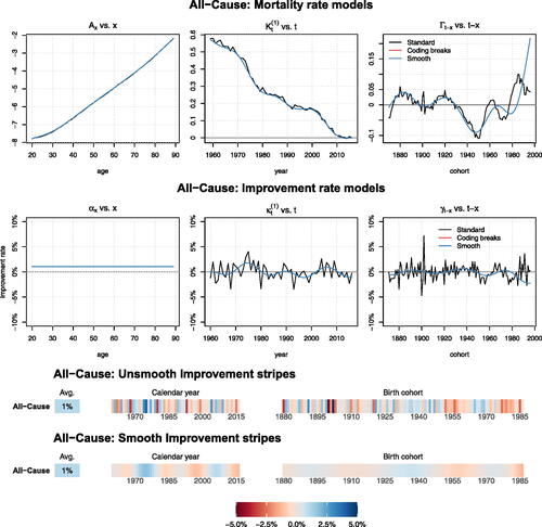
FIGURE 5. Fitted Parameters for the PCi Model for Mortality from Hypertensive Disease, Females, 1959–2016, Ages 20–89.

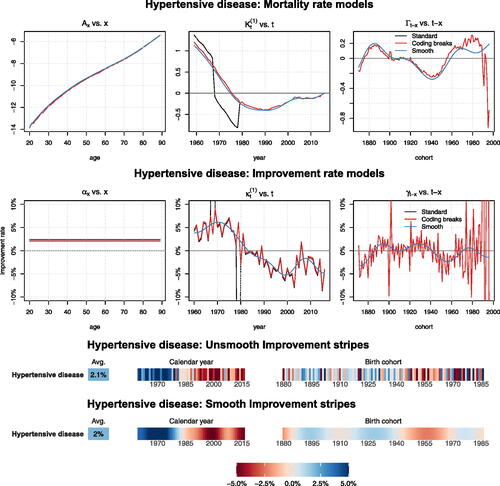
In Figures 4 and 5 we show for the corresponding cause of death the parameter estimates associated with the “standard” PCi model defined by Equation (2)(2) $$\hspace{0.17em}\mathrm{\text{log}}\hspace{0.17em}{m}_{x,t}=A_x+K_t+{\Gamma }_{t-x},$$(2) , the PCi model allowing for “coding breaks” defined by Equation (4)(4) $$\hspace{0.17em}\mathrm{\text{log}}\hspace{0.17em}{m}_{x,t}=A_x+K_t+{\Gamma }_{t-x}+\sum _{i=1}^h{\delta }_i{f}^{(i)}(t),$$(4) , and the “smooth” PCi model defined by Equation (5)(5) $$\hspace{0.17em}\mathrm{\text{log}}\hspace{0.17em}{m}_{x,t}=S_A(x)+S_K(t)+S_{\Gamma }(t-x)+\sum _{i=1}^h{\delta }_i{f}^{(i)}(t),$$(5) . For each of the models we present the fitted parameters in the mortality rate scale (top plots) and in the improvement rate scale (middle and bottom plots). Moreover, for the parameters in the improvement rate scales, we present two type of plots: traditional line plots and mortality improvement stripes. The latter type of plot is inspired by the “warming stripes” designed by Ed Hawkings (2018, 2023) to communicate temperatures change across the globe over the past century.

When presenting improvement rate parameters and to avoid possible identification issues associated with assigning main mortality improvements to period or cohort, we have reparameterized the PCi models in the following form: (6) $$\hspace{0.17em}\mathrm{\text{log}}\hspace{0.17em}\frac{m_{x,t}}{m_{x,t-1}}=\alpha +{\tilde{\kappa }}_t+{\tilde{\gamma }}_{t-x},$$(6) with $$\alpha =\frac{\sum _x\sum _t\left({\kappa }_t+{\gamma }_{t-x}\right)}{\sum _x\sum _{t}1},{\tilde{\kappa }}_t={\kappa }_t-\frac{\sum _t{\kappa }_t}{\sum _{t}1},\hspace{1em}\text{and}\hspace{1em}{\tilde{\gamma }}_{t-x}={\gamma }_{t-x}-\frac{\sum _x\sum _t{\gamma }_{t-x}}{\sum _x\sum _{t}1},$$ which is equivalent to imposing the constraints $\sum _t{\tilde{\kappa }}_t=0$ and $\sum _x\sum _t{\tilde{\gamma }}_{t-x}=0.$ Thus, $\alpha$ is interpreted as the average mortality improvement across all data cells and $\widetilde{{\kappa }_t}$ and ${\tilde{\gamma }}_{t-x}$ as the period and cohort deviations from this average improvement.

Figure 4 shows the results for all-cause mortality for females. These illustrative results are indicative of the type of discussion we can derive from the results of the different versions of the PCi model.

In the top row of Figure 4, we see that the parameters for the “standard” PCi model and the model with coding breaks coincide. This is because ICD coding changes do not affect mortality rates from all causes of death. We also see that the “smooth” version of the model follows closely the patterns of the standard model while smoothing out the year-on-year fluctuations in the period effect, $K_t,$ and in the cohort effect, ${\Gamma }_{t-x}.$

The middle row of Figure 4 presents the parameters in the improvement scale that are obtained by taking the first difference of the parameters in mortality rate scale (recall Eq. [3](3) $${\kappa }_t=-\Delta K_t=-(K_t-K_{t-1})\hspace{1em}\text{and}\hspace{1em}{\gamma }_c=-\Delta {\Gamma }_c=-({\Gamma }_c-{\Gamma }_{c-1}).$$(3) ). The advantages of the smoothing for the recognition of trends become more apparent in the improvement rate scale where year-on-year fluctuations are more evident.

The bottom row of Figure 4 depicts the improvement rate stripes, which is a more compact away of presenting the improvement rate parameters $\alpha ,$ ${\tilde{\kappa }}_t,$ and ${\tilde{\gamma }}_c.$ In the improvement stripes, the left panel labeled “Avg.” represents the parameter values of $\alpha ,$ the middle panel labeled “Calendar year” the period effects as captured by ${\tilde{\kappa }}_t,$ and the right panels labeled “Birth cohort” the cohort effects, ${\tilde{\gamma }}_c.$ The unsmooth improvement stripes corresponds to the black “standard” lines² in the middle row line plots, and the smooth stripes correspond to the blue “smooth” lines in the middle row plots. The values of the PCi model are mapped to a color so that blue hues signify mortality improvements and red hues signify mortality deterioration. We note that in the improvement rate stripes we have capped very large improvements and deteriorations at $\pm 5$% per annum (p.a.) so that very intense reds represent a deterioration of more than 5% p.a. and very intense blues represent improvements of more than 5% p.a. We also note that despite our estimation dataset covering cohorts born between 1871 and 1996, in our improvement stripe plots we only present parameter values of the cohort improvement deviations, ${\tilde{\gamma }}_{t-x},$ for cohorts born between 1881 and 1986. The oldest and youngest “corner” cohorts have only a limited number of observations, which can lead to erratic parameter estimates and discrepancies between smoothed and unsmoothed cohort effects.

From Figure 4 we note the following:

• The $\alpha$ parameter indicates that over the 1959 to 2016 period, all-cause mortality for females improved at an average pace of about 1.05% p.a.

• The ${\tilde{\kappa }}_t$ parameters represent period deviations from the average improvements, indicating that there are also clear period effects with all-cause mortality improving faster than average in the 1970s and late 2000s and slower than average in the 1960s, early 1980s, and after 2010. For example, the parameters of the “standard” PCi model show that ${\tilde{\kappa }}_{1975}=$4.04%, meaning that in 1975 all-cause mortality for females improved 4.04% p.a. more than the average of the whole period, for a total average model improvement rate of 5.08% p.a. in 1975. By contrast, the parameters of the “standard” unsmoothed PCi model show that ${\tilde{\kappa }}_{2015}=$ −2.3%, indicating that in 2015 all-cause mortality for females improved 2.3% p.a. less than the average of the 1959 to 2016 period, for a total average mortality deterioration of 1.25% p.a. in 2015.

• The ${\tilde{\gamma }}_c$ parameters, which represent cohort deviations from the average improvements, show that there are some clear cohort effects with the female cohorts born between 1925 and 1945 having above average improvements and the cohorts born between 1945 and 1960 having worse than average improvements. For example, in the “standard” PCi model we have that ${\tilde{\gamma }}_{1955}=$ –1.17%, indicating that females born in 1955 have experienced annual mortality improvements that are 1.17% worse than the average, for a total average deterioration of 0.13% p.a. for the 1955 cohort.

Figure 5 plots the results of fitting the PCi model to female mortality from hypertensive disease. We note that our estimation approach implies that the estimates of A_x, ${\Gamma }_{t-x},$ and ${\gamma }_{t-x}$ for the “Standard” and “Coding breaks” cases will always coincide and hence the corresponding lines in Figure 5 overlap. By contrast, in the estimates of K_t in the top middle panel of this figure, we see that allowing for coding breaks––through either model (4)(4) $$\hspace{0.17em}\mathrm{\text{log}}\hspace{0.17em}{m}_{x,t}=A_x+K_t+{\Gamma }_{t-x}+\sum _{i=1}^h{\delta }_i{f}^{(i)}(t),$$(4) or model (5)(5) $$\hspace{0.17em}\mathrm{\text{log}}\hspace{0.17em}{m}_{x,t}=S_A(x)+S_K(t)+S_{\Gamma }(t-x)+\sum _{i=1}^h{\delta }_i{f}^{(i)}(t),$$(5) ––effectively corrects for the very clear jump in mortality rates rates during the transitions from ICD-7 to -8 and from ICD-8 to -9.

5. AN ANALYSIS OF MORTALITY CHANGE IN THE UNITED STATES, 1959–2016

In this section we integrate epidemiological evidence with the application of the life expectancy decomposition methods and the PCi model introduced in the previous sections to construct a narrative of mortality change in the United States between 1959 and 2016, emphasizing the key drivers of this change and the features that characterize different time periods and generations.

Table 4 shows the contribution of different causes of deaths to the change in life expectancy at age 20 between 1959 and 2016 and five subperiods obtained using the decomposition approach introduced in Section 3.³ Figures 6 and 7 show for women and men aged 20 to 89, respectively, the results of applying the smooth PCi model for causes of death at the two levels of disaggregation defined in Table 2. Figure 8 shows equivalent decompositions for each risk factor defined in Table 3. The first two columns of Table 5 report the corresponding cause-specific average improvement rates over the study period; that is, parameter α in model (6)(6) $$\hspace{0.17em}\mathrm{\text{log}}\hspace{0.17em}\frac{m_{x,t}}{m_{x,t-1}}=\alpha +{\tilde{\kappa }}_t+{\tilde{\gamma }}_{t-x},$$(6) . The rest of the columns in Table 5 show the average period deviations in improvements for five subperiods, calculated as the average of ${\tilde{\kappa }}_t$ for the years in the subperiod. Similarly, Table 6 shows the corresponding average cohort deviations in mortality improvements for five cohort groups, calculated as the average of ${\tilde{\gamma }}_c$ for the cohorts in the group.⁴

FIGURE 6. Smooth Improvement Stripes for Causes of Death, Females, 1959–2016, Ages 20–89.

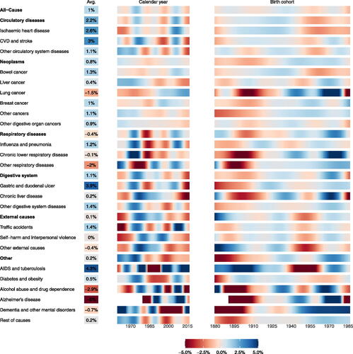
FIGURE 7. Smooth Improvement Stripes for Causes of Death, Males, 1959–2016, Ages 20–89.

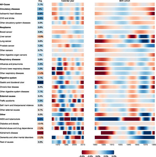
FIGURE 8. Smooth Improvement Stripes for Risk Factors, 1959–2016, Ages 20–89.

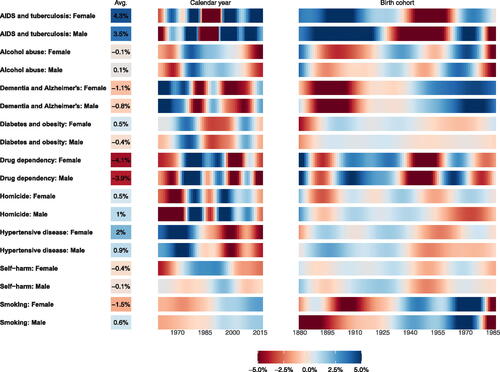
TABLE 4 Summary of Contribution to Life Expectancy Change at Age 20 for Different Subperiods

Cause	Study period		Subperiods
	1959–2016		1959–1970		1970–1980		1980–1995		1995–2010		2010–2016
	Female	Male	Female	Male	Female	Male	Female	Male	Female	Male	Female	Male
All-cause	6.31	7.44	0.93	–0.24	2.18	2.19	1.15	2.06	1.87	3.42	0.18	0.01
Circulatory diseases	6.29	6.23	0.99	0.45	1.8	1.74	1.63	1.94	1.65	1.92	0.22	0.18
Ischemic heart disease	3.34	4.31	–0.35	–0.26	1.07	1.26	1.2	1.6	1.18	1.46	0.24	0.25
CVD and stroke	1.65	1.08	0.31	0.15	0.6	0.4	0.37	0.24	0.33	0.27	0.03	0.02
Other circulatory system diseases	1.3	0.84	1.03	0.56	0.13	0.08	0.06	0.1	0.14	0.19	–0.05	–0.09
Neoplasms	0.85	1.04	0.07	–0.21	–0.04	–0.11	–0.04	0.19	0.63	0.83	0.24	0.34
Bowel cancer	0.28	0.18	0.04	0	0.05	0.01	0.08	0.05	0.09	0.09	0.02	0.03
Liver cancer	0.03	–0.06	0.05	0.03	–0.01	–0.01	0	–0.02	–0.01	–0.04	–0.01	–0.01
Lung cancer	–0.32	0.32	–0.11	–0.22	–0.19	–0.11	–0.24	0.1	0.09	0.36	0.12	0.19
Breast cancer	0.25	0	–0.03	0	0.02	0	0.04	0	0.18	0.01	0.04	0
Prostate cancer	0	0.13	0	0	0	–0.01	0	–0.01	0.01	0.13	0	0.03
Other cancers	0.5	0.25	0.08	–0.06	0.07	–0.04	0.05	0.02	0.25	0.23	0.06	0.09
Other digestive organ cancers	0.12	0.21	0.04	0.05	0.02	0.05	0.03	0.06	0.03	0.05	0	0.01
Respiratory diseases	–0.23	0.27	–0.04	–0.15	0.06	0.16	–0.27	0.03	0.02	0.18	0	0.04
Influenza and pneumonia	0.27	0.31	0.01	–0.02	0.19	0.21	–0.01	0.02	0.07	0.09	0.01	0.02
Chronic lower respiratory disease	–0.4	–0.03	–0.02	–0.07	–0.12	–0.1	–0.23	0.01	–0.03	0.1	0.01	0.03
Other respiratory diseases	–0.11	–0.01	–0.03	–0.05	–0.01	0.05	–0.03	0	–0.02	–0.01	–0.02	–0.01
Digestive system	0.18	0.27	–0.04	–0.07	0.1	0.13	0.12	0.17	0.03	0.06	–0.03	–0.02
Gastric and duodenal ulcer	0.05	0.12	0.01	0.04	0.02	0.05	0.01	0.02	0.01	0.02	0	0
Chronic liver disease	0.03	0.06	–0.07	–0.11	0.06	0.07	0.07	0.1	0	0.03	–0.03	–0.03
Other digestive system diseases	0.1	0.09	0.02	–0.01	0.02	0.01	0.04	0.06	0.01	0.01	0	0.01
External causes	–0.13	–0.08	–0.15	–0.35	0.17	0.21	0.14	0.45	–0.11	0.04	–0.17	–0.44
Traffic accidents	0.14	0.44	–0.06	–0.09	0.13	0.31	0.03	0.15	0.05	0.08	0	–0.01
Self–harm and interpersonal violence	–0.01	–0.11	–0.08	–0.16	0.03	–0.06	0.06	0.1	0.02	0.09	–0.03	–0.08
Other external causes	–0.26	–0.42	–0.02	–0.1	0.02	–0.03	0.06	0.2	–0.18	–0.13	–0.14	–0.35
Other	–0.66	–0.29	0.11	0.09	0.09	0.06	–0.44	–0.73	–0.35	0.38	–0.08	–0.09
AIDS and tuberculosis	0.06	0.12	0.05	0.08	0	0.02	–0.14	–0.59	0.13	0.58	0.01	0.03
Diabetes and obesity	0.1	–0.09	0	–0.03	0.1	0.04	–0.06	–0.07	0.07	0.01	–0.01	–0.04
Alcohol abuse and drug dependence	–0.03	–0.04	–0.01	–0.03	–0.01	0	0	0.01	0	0.02	–0.02	–0.03
Alzheimer’s disease	–0.34	–0.12	0	0	–0.01	–0.01	–0.12	–0.05	–0.13	–0.04	–0.08	–0.02
Dementia and other mental disorders	–0.29	–0.13	0	0	–0.04	–0.02	–0.03	–0.01	–0.27	–0.13	0.05	0.03
Rest of causes	–0.16	–0.02	0.07	0.06	0.05	0.04	–0.09	–0.01	–0.16	–0.06	–0.04	–0.06

TABLE 5 Departure of Mortality Improvement Rates from the Overall Average, by Subperiods and Causes of Death

Cause	Average improvement		Subperiod improvement above average
	Female	Male	1959–1970		1970–1980		1980–1995		1995–2010		2010–2016
			Female	Male	Female	Male	Female	Male	Female	Male	Female	Male
All-cause	1.04%	1.1%	–0.19%	–0.93%	1.17%	0.96%	–0.35%	–0.09%	0.02%	0.45%	–0.78%	–0.78%
Circulatory diseases	2.21%	2.01%	–0.63%	–1.39%	1.1%	0.92%	–0.3%	0.18%	0.56%	0.82%	–1.33%	–1.47%
Ischemic heart disease	2.63%	2.58%	–2%	–2.01%	0.44%	0.58%	–0.39%	0.26%	1.39%	1.1%	0.46%	–0.68%
CVD and stroke	2.97%	2.65%	–0.37%	–1.33%	2.26%	2.26%	–0.52%	–0.53%	0.18%	0.74%	–2.21%	–1.83%
Other circulatory system diseases	1.05%	0.55%	1.93%	0.59%	0.58%	0.11%	–0.56%	–0.1%	–0.3%	0.42%	–2.35%	–2.05%
Neoplasms	0.82%	0.78%	0.5%	–0.56%	–0.12%	–0.48%	–0.54%	–0.29%	0.29%	0.82%	–0.09%	0.51%
Bowel cancer	1.25%	0.8%	–0.15%	–1.1%	–0.7%	–1.39%	–0.22%	–0.33%	0.6%	1.51%	0.49%	1.38%
Liver cancer	0.45%	–0.91%	2%	1.27%	1.5%	0.73%	–0.62%	–1%	–0.96%	–0.51%	–2.22%	0.25%
Lung cancer	–1.51%	0.6%	–1.54%	–1.46%	–1.83%	–0.82%	–0.23%	0.06%	1.58%	0.95%	2.49%	1.52%
Breast cancer	1.03%	–	–0.46%	–	–0.34%	–	–0.28%	–	0.85%	–	–0.02%	–
Prostate cancer	–	1.17%	–	–0.19%	–	–1.2%	–	–1.55%	–	2.19%	–	0.75%
Other cancers	1.13%	0.68%	1.07%	–0.17%	0.56%	0.17%	–0.68%	–0.39%	–0.11%	0.42%	–0.92%	–0.03%
Other digestive organ cancers	0.85%	0.98%	0.7%	0.52%	0.26%	0.28%	0.02%	0.03%	–0.34%	–0.23%	–0.91%	–0.9%
Respiratory diseases	–0.38%	0.56%	0.07%	–0.68%	1.04%	1.59%	–1.74%	–0.62%	0.86%	0.24%	0.33%	–0.45%
Influenza and pneumonia	1.16%	1.44%	0.69%	0.13%	2.46%	2.11%	–2.5%	–1.92%	0.67%	0.78%	–0.78%	–0.9%
Chronic lower respiratory disease	–0.11%	1.2%	0.96%	–1.88%	4.56%	6.83%	–2.81%	–1.64%	–0.69%	–1.12%	–0.61%	–1.05%
Other respiratory diseases	–2.01%	–1.4%	1.79%	2.53%	–5.02%	–5.33%	0.6%	1.08%	1.41%	0.81%	0.06%	–0.48%
Digestive system	1.15%	1.14%	–0.74%	–1.33%	2.66%	2.01%	0.5%	0.81%	–0.68%	–0.34%	–2.62%	–2.07%
Gastric and duodenal ulcer	3.93%	4.93%	0.14%	1.04%	1.75%	3.61%	–1.06%	–1.43%	1.21%	0.46%	–3.57%	–5.48%
Chronic liver disease	0.24%	0.41%	–1.85%	–2.86%	3.15%	2.19%	1.91%	1.88%	–0.75%	0.08%	–4.76%	–3.3%
Other digestive system diseases	1.36%	1.12%	0.39%	–0.72%	2.59%	1.83%	–0.53%	0.15%	–1%	–0.68%	–1.2%	–0.41%
External causes	0.05%	0.44%	–2.31%	–2.06%	2.97%	2.76%	1.68%	1.52%	–1.01%	–0.59%	–2.36%	–3.15%
Traffic accidents	1.36%	1.51%	–3.96%	–3.05%	2.9%	3.09%	–0.83%	1.15%	1.38%	–0.64%	1.06%	–0.83%
Self–harm and interpersonal violence	0.01%	0.3%	–3.21%	–2.43%	1.05%	0.44%	2.19%	1.11%	0.37%	0.88%	–2.26%	–1.24%
Other external causes	–0.43%	0.05%	–1.84%	–1.53%	3.4%	3.92%	1.94%	2.18%	–2.01%	–1.99%	–2.09%	–4.18%
Other	0.18%	0.17%	2.82%	1.86%	3.05%	2.35%	–1.33%	–2.03%	–2.23%	–0.45%	–1.35%	–1.12%
AIDS and tuberculosis	4.28%	3.55%	1.12%	–1.14%	3.39%	6.08%	–10.65%	–15.13%	5.16%	10.16%	6.01%	4.39%
Diabetes and obesity	0.53%	–0.35%	0.63%	–0.3%	2.9%	3.55%	–2.53%	–1.98%	0.22%	0.08%	–0.23%	–0.62%
Alcohol abuse and drug dependence	–2.9%	–1.18%	–2.29%	–2.75%	1.67%	1.9%	2.23%	1.59%	0.43%	1.3%	–5.24%	–5.35%
Alzheimer’s disease	–6.47%	–4.31%	–	–	–18.53%	–17.52%	–2.57%	–1.73%	2.94%	2.53%	2.17%	0.93%
Dementia and other mental disorders	–0.72%	–1.16%	7.84%	4.76%	1.24%	–0.51%	0.53%	1.72%	–8.22%	–6.1%	2.78%	3.06%
Rest of causes	0.16%	0.27%	2.21%	1.56%	1.42%	1.12%	–0.59%	–0.09%	–1.59%	–1.3%	–0.96%	–1.28%
Risk factors
AIDS and tuberculosis	4.28%	3.55%	1.12%	–1.14%	3.39%	6.08%	–10.65%	–15.13%	5.16%	10.16%	6.01%	4.39%
Smoking	–1.51%	0.6%	–1.54%	–1.46%	–1.83%	–0.82%	–0.23%	0.06%	1.58%	0.95%	2.49%	1.52%
Diabetes and obesity	0.53%	–0.35%	0.63%	–0.3%	2.9%	3.55%	–2.53%	–1.98%	0.22%	0.08%	–0.23%	–0.62%
Alcohol abuse	–0.06%	0.08%	–1.96%	–2.78%	2.87%	2.03%	1.91%	1.8%	–0.57%	0.2%	–4.56%	–3.29%
Drug dependency	–4.13%	–3.85%	–3.02%	–3.35%	4.61%	7.19%	3.95%	1.73%	–4.07%	–2.04%	–1.84%	–5.07%
Dementia and Alzheimer’s disease	–1.12%	–0.78%	6.75%	5.89%	1.75%	–0.41%	–1.99%	–0.88%	–4.47%	–3.53%	0.86%	0.89%
Hypertensive disease	2.03%	0.92%	4.93%	3.38%	4.43%	4.39%	–1.43%	–0.89%	–3.52%	–3.23%	–4.05%	–3.22%
Self–harm	–0.38%	–0.12%	–2.59%	–0.01%	1.36%	–0.67%	2.84%	0.6%	–0.91%	0.13%	–2.34%	–0.69%
Homicide	0.52%	0.99%	–4.4%	–7.67%	0.38%	1.23%	1.12%	2%	2.19%	3.16%	–0.84%	–0.89%

TABLE 6 Departure of Mortality Improvement Rates from the Overall Average, by Cohort Group and Causes of Death

Female cohort:	1881–1925		1925–1945		1945–1960		1960–1975		1975–1986
Male cohort:	1881–1920		1920–1940		1940–1955		1955–1970		1970–1986
Cause	Female	Male	Female	Male	Female	Male	Female	Male	Female	Male
All-cause	0.01%	–0.29%	0.48%	0.84%	–0.44%	–0.69%	–0.07%	–0.05%	–0.44%	–0.59%
Circulatory diseases	0.33%	0.06%	0.74%	1.24%	–1.23%	–0.3%	–1.21%	–1.03%	–0.68%	–2.65%
Ischemic heart disease	0.51%	–0.36%	0.85%	1.25%	–1.38%	0.02%	–1.83%	–0.14%	–1.39%	–3.19%
CVD and stroke	0.03%	0.38%	0.15%	0.47%	–0.81%	–1.04%	0.4%	–0.43%	0.09%	–0.51%
Other circulatory system diseases	0.03%	0.41%	0.68%	1.11%	–0.88%	–1.02%	–0.59%	–1.3%	0.68%	–0.82%
Neoplasms	–1.11%	–1.26%	0.52%	0.35%	1.04%	0.49%	0.94%	1.19%	0.42%	0.19%
Bowel cancer	0.1%	0.33%	0.98%	0.84%	–0.93%	–0.49%	–1.61%	–1.99%	–0.91%	–0.47%
Liver cancer	–0.17%	–0.14%	–0.08%	0.43%	–0.72%	–3.89%	1.44%	4.54%	0.25%	0.24%
Lung cancer	–2.42%	–3.26%	1.2%	0.66%	1.8%	1.96%	6.02%	3.95%	–0.44%	–0.94%
Breast cancer	–0.97%	–	0.31%	–	1.06%	–	0.25%	–	0.93%	–
Prostate cancer	–	–0.67%	–	0.92%	–	–1.59%	–	–0.43%	–	3.05%
Other cancers	–1.58%	–1.82%	0.65%	0.19%	1.15%	0.9%	0.7%	1.64%	0.64%	0.67%
Other digestive organ cancers	–0.24%	–0.02%	0.59%	0.15%	0.02%	0.22%	0.07%	0.69%	–0.57%	–1.5%
Respiratory diseases	–0.74%	–1.72%	–0.13%	0.76%	0.73%	0.24%	2.11%	1.28%	1.83%	0.04%
Influenza and pneumonia	–0.26%	–0.98%	–0.49%	0.75%	0.26%	–0.74%	0.7%	1.36%	–0.15%	–1.16%
Chronic lower respiratory disease	–2.91%	–2.74%	1.16%	1.46%	1.01%	0.86%	3.6%	0.65%	3.7%	–0.18%
Other respiratory diseases	–1.9%	–2.82%	0.4%	1.27%	0.72%	0.11%	1.64%	1.29%	2.15%	1.17%
Digestive system	–0.83%	–0.52%	0.64%	0.56%	–0.32%	–1.2%	1.9%	2.38%	0.05%	–0.6%
Gastric and duodenal ulcer	–1.16%	–1.22%	0.44%	1.16%	–0.14%	–0.91%	0.83%	1.04%	1.16%	–0.27%
Chronic liver disease	–1.77%	–0.84%	1.85%	0.55%	–0.63%	–1.12%	3.56%	3.28%	–0.7%	–0.85%
Other digestive system diseases	–0.59%	–0.51%	–0.1%	0.43%	0.09%	–1.16%	1.27%	1.9%	0.78%	–0.13%
External causes	0.87%	0.19%	0.16%	0.44%	–2.1%	–1.57%	0.43%	0.16%	0.58%	0.35%
Traffic accidents	–0.2%	0.1%	0.33%	–0.14%	–0.88%	–1.04%	0.51%	0.38%	–0.17%	1.16%
Self–harm and interpersonal violence	–0.12%	0.35%	0.42%	0.57%	–1.4%	–1.11%	0.76%	–0.67%	0.3%	–0.45%
Other external causes	1.93%	0.44%	0.27%	0.89%	–3.38%	–2.42%	–0.41%	0.34%	–0.62%	–0.3%
Other	–2.18%	–1.56%	0.97%	0.28%	0.03%	–1.61%	2.44%	3.42%	2.17%	2.35%
AIDS and tuberculosis	3.88%	6.94%	–1.21%	–2.31%	–7.21%	–7.88%	0.85%	–0.12%	1.72%	0.16%
Diabetes and obesity	–0.04%	0.03%	0.53%	0.34%	–0.58%	–0.44%	–1.08%	–0.15%	–0.07%	–0.25%
Alcohol abuse and drug dependence	–3.18%	–2.16%	2.12%	0.61%	–0.77%	–1.55%	4.27%	4.02%	–0.99%	0.94%
Alzheimer’s disease	–5.82%	–7.29%	0.99%	0.4%	1.68%	1.92%	5.56%	1.67%	–2.53%	3.14%
Dementia and other mental disorders	–4.97%	–5.4%	–0.06%	–0.27%	3.66%	1.92%	4.52%	4.38%	4.66%	5.41%
Rest of causes	–1.48%	–1.19%	0.12%	0.36%	0.72%	–1.03%	1.57%	2.23%	1.14%	1%
Risk factors
AIDS and tuberculosis	3.88%	6.94%	–1.21%	–2.31%	–7.21%	–7.88%	0.85%	–0.12%	1.72%	0.16%
Alcohol abuse	–1.53%	–0.68%	1.88%	0.65%	–0.67%	–1.06%	3.29%	2.75%	–1.83%	–1.38%
Dementia and Alzheimer’s disease	–3.61%	–3.79%	0%	–0.11%	2.94%	1.44%	4.16%	3.55%	4.17%	4.92%
Diabetes and obesity	–0.04%	0.03%	0.53%	0.34%	–0.58%	–0.44%	–1.08%	–0.15%	–0.07%	–0.25%
Drug dependency	1.13%	1.73%	–0.01%	0.14%	–4.78%	–6.04%	1.64%	3.2%	–2.14%	–2.17%
Homicide	–0.71%	0.38%	0.91%	0.7%	–1.25%	0.3%	0.68%	–2.09%	0.54%	–2.49%
Hypertensive disease	0.52%	1.4%	0.75%	0.77%	–1.96%	–1.89%	–0.62%	–1.4%	0.23%	–1.1%
Self–harm	0.11%	0.29%	0.28%	0.86%	–1.09%	–1.89%	0.64%	–0.32%	–0.77%	–0.1%
Smoking	–2.42%	–3.26%	1.2%	0.66%	1.8%	1.96%	6.02%	3.95%	–0.44%	–0.94%

Note: Cohort groups for women and men have different boundaries.

5.1. The Overall Trend in Mortality Improvements over 60 Years

In the left panels of Figures 6 and 7 and in the first two columns of Table 5, we see that in the period between 1959 and 2016 most causes of death experienced on average an improvement in mortality. Over the study period, the United States saw a remarkable reduction in mortality rates, with all-cause mortality rates for both women and men aged 20 to 89 improving at an average pace of around 1% p.a. The faster improvements occurred for circulatory diseases as a whole, IHD, CVD and stroke, gastric and duodenal ulcer, and AIDS and tuberculosis, where mortality for both genders improved at an average pace of more than 2% p.a. There are, however, some causes of death that are the exception and that experienced an overall deterioration of mortality. Particularly noteworthy are the sharp deteriorations in both male and female mortality from alcohol abuse and drug dependence, Alzheimer’s disease, and dementia and other mental disorders. Other causes where mortality deteriorated include liver cancer and diabetes for males, lung cancer for females, and other respiratory diseases for both genders.

Whereas the first half of the 20th century was dominated by improvements in mortality from infectious diseases, the story of mortality evolution in the United States in the second half of the 20th century that continued into the first decade of the 21st century has been mainly a story of mortality improvements from circulatory diseases. In fact, in Table 4 we see that 6.29 years of the 6.31-year increase in life expectancy at age 20 for females over the study period can be attributed to reductions in mortality rates from circulatory causes of death. Overall, the increase in life expectancy for men was larger than for women, but the magnitude of the gain attributable to a decline in circulatory diseases (6.23 years) was of a similar scale.

The improvement in mortality from circulatory diseases can be linked to both a delayed onset of disease due to improvements in the prevalence of cardiovascular risk factors such as hypertension, high cholesterol and smoking and reductions in case fatality with the introduction of novel surgical and pharmacological treatments (Mensah et al. 2017). For ischemic heart disease in particular, Ford et al. (2007) estimated that 47% of the decrease in mortality rates between 1980 and 2000 can be attributed to improved uptake of evidence-based medical and surgical treatments and the net reduction in the prevalence of major risk factors accounted for 44% of the decrease.⁵ Notably, Ford et al. (2007) reported that increases in body mass index and diabetes have partially offset some of the gains.

Nevertheless, despite the clear dominance of circulatory diseases as a leading cause of death and as the main contributor to mortality improvements over the study period, the decline of mortality has been more complex. The trajectories of other major causes have ebbed and flowed, and the patterns of behavioral risk factors saw changes between generations.

5.2. Subperiods of Mortality Improvement

We see in the middle panels of Figures 6, 7, and 8 that most causes of death and risk factors exhibit a clear period effect, with similar patterns observed in females and males. We can identify five broad periods of mortality change, which are summarized in Tables 4 and 5.

5.2.1. 1959–1970

The first period comprises the years between 1959 and 1970 in which life expectancy at age 20 for women showed a small increase from 55.75 to 56.68 years and for men decreased from 49.82 to 49.58 years. During this period, all-cause mortality improved very slowly for women and stagnated for men as a result of the below-average improvements (or deterioration) in mortality for the majority of the causes. This resulted in a general leveling off in mortality rates after the unprecedented decline in mortality experienced by Americans from 1940 to the mid-1950s (Crimmins 1981). Some key features of this period are as follows:

• The 1960s were the first decade in which a decline in mortality rates from circulatory diseases as a whole started to become evident after mortality rates from this cause had reached a peak in the 1950s (Centers for Disease Control and Prevention 1999a).

• However, despite the overall fall in cardiovascular mortality rates, the rate of mortality improvements in the 1960s were sluggish, mainly due to the increase in mortality rates from IHD (the dominant group of cardiovascular deaths), which only achieved peak mortality rates in the mid-1960s (Centers for Disease Control and Prevention 1999a). In fact, IHD accounted for 0.35 years and 0.26 years of life expectancy deterioration between 1959 and 1970 for females and males, respectively (Table 4).

• Lung cancer was another major contributor to mortality deterioration during this period, accounting for a fall of 0.11 years and 0.22 years in life expectancy for females and males, respectively (Table 4). This is in line with the noticeable negative period effects in rates of improvement, where we see that lung cancer improvement rates fell to 1.54% p.a. and 1.46% p.a. below the average for women and men, respectively (Table 5).

• External causes of death also played a central role, contributing 0.15 and 0.35 years to the deterioration of life expectancy for females and males, respectively, during this period (Table 4). Among the external causes, the negative contribution of self-harm and interpersonal violence is noteworthy.

5.2.2. 1970–1980

After the slow mortality improvements of the 1960s, mortality trends in the United States experienced a turning point around 1968, with mortality decline accelerating thereafter (Crimmins 1981; Ouellette, Barbieri, and Wilmoth 2014), with the 1970s being the decade of the fastest all-cause mortality improvements over the study period. This very fast decline in mortality rates translated into life expectancy at age 20 increasing from 55.68 to 58.86 years for women and from 49.58 to 51.77 years for men over the decade 1970 to 1980. The key features of this period are as follows:

• The turning point in all-cause mortality trends coincides with the turning point in mortality trends from circulatory causes of death seen in 1971 that marked the beginning of rapid declines in mortality from circulatory diseases (Ouellette, Barbieri, and Wilmoth 2014). This revolution in mortality improvements from circulatory diseases in the 1970s was the result of reductions in lifestyle risk factors such as cholesterol levels and smoking, as well as major advances in medical treatments such as prehospital resuscitation, coronary artery bypass surgery, and the treatment of hypertension (Goldman and Cook 1984).

• Importantly, the 1970s was the decade in which cigarette consumption in the United States started to decrease steadily. After increasing rapidly for much of the first part to the 20th century, cigarette consumption reached a plateau in the 1960s and early 1970s following the influential first report of the Surgeon General’s Committee on Smoking and Health in 1964 establishing a causal link between smoking and lung cancer, resulting in the introduction of anti-smoking ads in 1969 and a ban on cigarette commercials on TV and radio in 1971. From 1973 onwards, cigarette consumption decreased steadily as a result of the so-called nonsmoker movement, which led to legislation banning smoking in several public places (Garfinkel 1997; Centers for Disease Control and Prevention 1999c).

• However, despite the general decline in smoking prevalence in the 1970s, lung cancer continued its important negative contribution to mortality change. This is because period trends in lung cancer are mainly determined by the changes in cigarette consumption with a 20 to 30 year lag (Crimmins 1981).

• After circulatory diseases, traffic accidents and influenza and pneumonia were the two other major contributors to the decline in mortality in the 1970s. On the one hand, death rates from traffic accidents decreased significantly during this period after having peaked in the late 1960s. This decline in traffic accident fatalities followed the passage in 1966 of the Highway Safety Act and the National Traffic and Motor Vehicle Safety Act, which authorized the federal government to set and regulate standards for motor vehicles and highways (Centers for Disease Control and Prevention 1999b). On the other hand, after having leveled off between 1950 and 1960, mortality rates from influenza and pneumonia fell sharply in the 1970s until reaching a turning point in 1980 when they started to rise again (Armstrong, Conn, and Pinner 1999).

5.2.3. 1980–1995

Over the period 1980 to 1995 mortality improvements continued, although at a much slower pace than in the 1970s. Between 1980 and 1995, life expectancy at age 20 for women increased from 58.86 years to 60.01 years, and for men it increased from 51.77 years to 53.83 years. The key drivers of the slower improvements during this period are as follows:

• After having decreased steadily during the 20th century, mortality rates from infectious diseases started to rise unexpectedly in the 1980s driven by an increase in mortality rates from influenza and pneumonia and, more important, by the emergence of the AIDS/HIV epidemic in the early 1980s (Armstrong, Conn, and Pinner 1999). AIDS/HIV would become one of the main drivers of the slowdown in mortality improvements, with AIDS and tuberculosis accounting for 0.14 years and 0.59 years of deterioration in life expectancy between 1980 and 1995 for females and males, respectively (Table 5).

• For women, the other major contributors to slower mortality improvement were smoking-related lung disease, with lung cancer and chronic lower respiratory diseases accounting, respectively, for 0.24 and 0.23 years of life expectancy deterioration in the 1980 to 1995 period (Table 5). Noticeably, this negative effect is seen for women but not for men, reflecting the historic differences in tobacco consumption patterns among men and women and the 20 to 30 year latency period for lung cancer and chronic lower respiratory diseases to manifest themselves (Crimmins 1981; Kazerouni et al. 2004). This is consistent with the fact that smoking prevalence for men peaked in the 1950s, whereas for women it peaked a decade later (Garfinkel 1997; Centers for Disease Control and Prevention 1999c).

• Circulatory diseases continued to show important mortality improvements, albeit at a slower pace than in the 1970s, partially because of the rising trends in the prevalence of obesity and diabetes (Ford and Capewell 2007). In particular, the prevalence of obesity among Americans aged 20 to 74 increased dramatically since the late 1970s, doubling from 15% in 1976–1980 to 30.9% in 1999–2000 (Fryar et al. 2012). Similarly, the prevalence of diagnosed diabetes among Americans aged 20 to 79 started to increase in the late 1980s, rising from 3.5% in 1990 to 8.3% in 2012 (Geiss et al. 2014). The key drivers of the so-called diabesity epidemic are multifactorial and include secular changes in agricultural policies, diet, food environment, physical inactivity, and sleep deprivation (Bhupathiraju and Hu 2016).

5.2.4. 1995–2010

After the slight slump in the pace of mortality improvements over the preceding 15 years, improvements accelerated from 1995 through to 2010, especially for men. As a result, period life expectancy rose in this period by a remarkable 3.42 years for men (from 53.83 years to 57.25 years) and by 1.87 years for women (from 60.01 years to 61.88 years). Some of the key features of mortality change in this period include the following:

• A continued improvement in circulatory disease mortality at a pace faster than the preceding period. However, between 1995 and 2010, an age divide in the pace of mortality improvements for circulatory diseases has been reported in the literature, with the mortality rates among young adults––and especially women––showing signs of stagnation, in sharp contrast with older Americans, who experienced steep mortality declines that accelerated from the early 2000s (Ford and Capewell 2007; Wilmot et al. 2015). This stagnation in circulatory disease mortality among younger adults coincides with a substantial deterioration in the 1980s and 1990s in the prevalence of major traditional risk factors such diabetes, obesity, and hypertension (Flegal et al. 1998; Fox et al. 2007).

• Noticeably, in this period mortality rates from neoplasms as a whole also started to experience sustained improvements after having peaked in the early 1990s (Edwards et al. 2010; Ouellette, Barbieri and Wilmoth 2014). Thus, neoplasms contributed 0.63 and 0.83 years to the increase in life expectancy at age 20 between 1995 and 2010 for females and males, respectively (Table 5), with much of this increase stemming from improvements in mortality from major cancers: lung, breast, and prostate cancer. Though cohort effects, especially related to smoking patterns, are behind much of the decrease in cancer mortality during this period, there are still some noteworthy period patterns. For lung cancer, both women and men show matching positive period effects starting from 1990, which, as discussed before, reflect with a 20 to 30 year lag the onset in the 1970s of a steady decrease in tobacco consumption following the 1964 Surgeon General’s reports on smoking and health. In the case of prostate cancer, mortality rates peaked in the early 1990s following the widespread introduction of prostate-specific antigen screening, with its subsequent benefits in terms of earlier detection. This, together with improved treatments, contributed to a continuing decline in prostate cancer mortality rates from the early 1990s to the early 2010s, which has nonetheless leveled off in recent years because of a decrease in the uptake of prostate-specific antigen (Negoita et al. 2018). Similarly, after a period of stable mortality rates in the 1980s, breast cancer mortality started to decrease steadily in the early 1990s. Though this decline coincides with the introduction of mammography screening in the late 1980s and early 1990s, the impact of mammographies on the reduction of mortality remains contentious: it is argued that the decline is more likely attributable to an increase in the detection of smaller palpable tumors and to the increase in the use of adjuvant chemotherapy (Jatoi and Miller 2003; Narod, Iqbal, and Miller 2015).

• After the dramatic negative impact of the HIV epidemic in the 1980s, this period showed a sharp decline in the incidence and mortality from AIDS coinciding with the introduction of anti-retroviral therapy in 1996 (Murphy et al. 2001).

• In contrast to these positive trends, this period saw the emergence of Alzheimer’s disease, dementia, and other mental disorders as a very important cause of mortality, especially among women. In fact, between 1995 and 2010, Alzheimer’s and dementia combined contributed to a fall in life expectancy at age 20 by 0.40 years and 0.27 years for women and men, respectively (Table 5). One explanation for the mortality increase is the improved clinical awareness and diagnosis of Alzheimer’s and dementia (Weuve et al. 2014). However, with population aging and mortality from major causes in decline, more people are surviving to ages where the risk of Alzheimer’s and dementia is highest, explaining in part the observed increase (Kramarow and Tejada-Vera 2019).

• Mortality rates from other external causes of death also experienced a significant increase during this period, with a significant portion of this mortality deterioration coming from an increase in mortality rates from unintentional drug poisoning linked to prescribed opioid use (Alexander, Kiang, and Barbieri 2018; Masters, Tilstra, and Simon 2018). This increase foreshadowed the narrative of “deaths of despair” that would come to dominate the discussion of U.S. mortality change in the 2010s.

5.2.5. 2010–2016

Starting from around 2010, overall mortality improvements in the United States showed a considerable slowdown leading to a stagnation in life expectancy. For women, between 2010 and 2016 life expectancy at age 20 increased by only 0.18 years, rising from 61.88 years in 2010 to 62.06 years in 2016. For men, the slowdown in mortality improvements resulted in life expectancy increasing minimally from 57.25 years in 2010 to 57.26 years in 2016. Some of the key drivers behind this slowdown in improvements are discussed below:

• The main narrative behind the slowdown of mortality improvements after 2010 has been that of “deaths of despair” popularized by the widely cited paper by Case and Deaton (2015). They argued that the slowdown of mortality improvement was mainly due to an increase in accidental drug and alcohol poisoning, chronic liver disease, cirrhosis, and suicide, especially among middle-aged white Americans. In a follow-up paper, Case and Deaton (2017) argued that these deaths of despair are a cohort effect resulting from the cumulative decline in living standards across generations. However, this “deaths of despair” narrative has been challenged. Masters, Tilstra, and Simon (2018) suggested that much of the change is due to period rather than cohort effects linked to an increase in drug-use related mortality associated with opioids. Harper et al. (2020) argued that though opioids are one of the key drivers of the slowdown of improvements, there are other causes of death that have contributed, including increases in mortality from Alzheimer’s disease, homicide, and suicide, together with a slowdown in mortality improvements from circulatory diseases.

• Our modeling results support the complementary findings of Case and Deaton (2015) and Harper et al. (2020) in relation to the diversity of causes driving the stagnation of mortality improvements. Moreover, in agreement with Masters, Tilstra, and Simon (2018), the results of our APC decomposition suggest that period effects play a central role. In particular, in the last two columns of Table 5, we report large negative period effects for circulatory diseases, chronic liver disease, self-harm, and interpersonal violence and, notably, from deaths linked to alcohol abuse and drug dependency.

• Circulatory diseases remain the leading cause of death in the 21st century. In Table 5, we see that during this period mortality from circulatory diseases for women and men, respectively, experienced improvements that were 1.33% p.a. and 1.47% p.a. slower than the average 2.21% p.a. and 2.01% p.a. over the whole study period. This resulted in net improvements of just 0.88% p.a. and 0.54% p.a. between 2010 and 2016 for women and men, respectively. Mehta, Abrams, and Myrskylä (2020) argued that this slowdown in the pace of mortality improvements for circulatory diseases could even be the main driver for the stagnation in life expectancy as opposed to the counternarrative of deaths of despair. Some of the preliminary potential explanations for the stagnation of improvements include the increase in the prevalence of diabetes and obesity, the plateauing of the benefits of the decrease in smoking prevalence, and the fact that advancements in the treatment and prevention of circulatory diseases have become more incremental in recent years (Sidney et al. 2016; Mensah et al. 2017; Mehta, Abrams, and Myrskylä 2020).

5.3. Cohort Effects

In contrast to period effects where both genders have similar patterns, we see in the right panels of Figures 6, 7, and 8 that there are contrasting patterns in the mortality improvements for females and males along the cohort dimension. In particular, the brighter intensity of the red and blue stripes for males indicates more marked cohort effects for men than for women. In addition, the boundaries of the cohort groups with similar behaviors differ slightly between the genders, reflecting the delayed onset of common risk factors among women. On visual inspection of the birth cohort panels in Figures 6, 7, and 8, we identify for men five broad cohort groups encompassing the generations born in 1881–1920, 1920–1940, 1940–1955, 1955–1970 and 1970–1986, whereas for women these cohort groups are 1881–1925, 1925–1945, 1945–1960, 1960–1975, and 1975–1986. Table 6 summarizes the deviation of mortality improvements for each cohort above or below the overall average improvement over the study period.

5.3.1. Females 1881–1925, Males 1881–1920

This cohort group shows average mortality improvements for women and slightly below-average improvements for men corresponding, respectively, to all-cause cohort effects of 0.01% p.a. and –0.29% p.a. (Table 6). These below-average improvements are mainly explained by patterns of cigarette consumption among this generation, as reflected by the large negative cohort effects that both genders show for lung cancer and chronic lower respiratory diseases. In particular, Preston and Wang (2006) reported that cigarette consumption (in terms of average number of years spent as a cigarette smoker before age 40) increased steadily from the 1885–1889 generation to reach a plateau for the 1910–1925 generation of men and the 1925–1940 generation of women.

5.3.2. Females 1925–1945, Males 1920–1940

This cohort group shows above average-mortality improvement, with women having a positive cohort effect of 0.48% p.a. and men a positive cohort effect of 0.84% p.a., stemming from positive cohort effects for the majority of causes of death and most risk factors (Table 6). Some key characteristics of this cohort include the following:

• This is the first generational group that does not show an increase in smoking prevalence relative to the preceding generations. Moreover, from this generation onwards cigarette consumption decreased steadily (Harris 1983; Preston and Wang 2006).

• This generation shows a clear positive cohort effect in alcohol-related mortality. In the particular case of men, this is consistent with the strong declining trend in alcohol volume consumption and frequency of heavy drinking reported by Kerr et al. (2009) for those born between 1920 and 1940.

• In contrast to the positive cohort effects from other risk factors, this generation, who were in their 40s to 60s in the 1980s, shows negative cohort effects from AIDS and tuberculosis, albeit milder than those seen in the following generation.

5.3.3. Females 1945–1960, Males 1940–1955

The generation of early baby boomers is noticeably one of the generations with the slowest mortality improvements among the generations included in the study. Women from this generation experience mortality improvements that are 0.44% p.a. below the average and men experience mortality improvement 0.69% p.a. below the average (Table 6). The reasons for the below-average improvement are multifactorial and reflect adverse patterns in a diverse number of causes and risk factors:

• As with the preceding generation, early baby boomers continued to experience positive cohort effects from smoking-related causes of death as a consequence of the continued decline in tobacco consumption among younger generations. However, the positive gains from smoking were counterbalanced by negative trends in other factors and causes.

• In particular, this generation marked the start of a turning point in generational patterns of circulatory disease mortality with cohorts born from around 1945 to 1950 onwards showing negative cohort effects for this group of causes. This pattern coincides with similar turning points in the mortality rates from markers of cardiovascular risk factors including hypertension, obesity and diabetes. In the case of obesity, though period effects tend to dominate when explaining trends in obesity prevalence, some cohort effects have also been reported, with obesity prevalence rising steadily for younger generations starting from the 1955 birth cohort (Reither, Hauser, and Yang 2009; An and Xiang 2016).

• Early baby boomers also show distinctive negative patterns in mortality rates associated with alcohol abuse and drug dependency. For drug dependency, the negative cohort effects coincide with the strong cohort patterns found by Kerr, Lui, and Ye (2018), who reported an important increase in marijuana consumption between the 1945 and 1955 generations. Moreover, heroin and pain reliever misuse were reported to show cohort patterns (Verdery et al., 2020), which match an increasing trend in prescription opioid and heroin overdose mortality among individuals born between 1947 and 1964 (Huang, Keyes, and Li 2018).

• This generation of men and women who were in their early and middle adulthood in the 1980s during the peak of the HIV epidemic exhibits a very strong negative cohort effect from AIDS even after controlling for period effects (Acosta et al., 2020).

• Finally, this cohort shows significant negative cohort effects for suicide that are consistent with the shift in cohort patterns in suicide rates that began to increase sharply for both genders starting from the baby boom generation (Phillips 2014).

5.3.4. Females 1960–1975, Males 1955–1970

This generation shows mortality improvements that are close to the average, with women and men experiencing minimal negative cohort effects of –0.07% p.a. and –0.05% p.a., respectively (Table 6). These average improvements reflect offsetting patterns for different causes and risk factors. Similar to the preceding generation, this generation continued the negative cohort effects from circulatory diseases, obesity and diabetes, and hypertension, consistent with the previously discussed increasing trend in obesity prevalence that started with the 1955 birth cohort. Likewise, this generation continues to benefit from the positive cohort effects stemming from reductions in smoking prevalence. However, in sharp contrast with the previous and subsequent generations, this cohort group shows positive cohort effects for alcohol abuse and drug dependency.

5.3.5. Females 1975–1986, Males 1970–1986

Together with the baby boomer generation, this youngest generation shows the worst mortality improvements among the cohorts in the study, with women showing worryingly negative cohort effects of –0.44% p.a. and men negative effects of –0.59% p.a. (Table 6). These negative effects reflect adverse patterns in several risk factors for this cohort:

• This cohort group shows important negative cohort effects for alcohol-related mortality. This is in line with several studies that reported a sharp increase in alcohol volume consumption and frequency of heavy drinking starting from the 1970 birth cohort until the 1985 cohort (Kerr et al. 2009, 2013). Similarly, Huang, Keyes, and Li (2018) reported an increasing trend in prescription opioid and heroin overdose mortality among those born between the start of the 1970s and the start of the 1980s.

• Noticeably, the positive cohort effects associated with smoking and lung cancer seem to be winding down, with women and men of this generation showing a negative cohort effect in lung cancer mortality of –0.44% p.a. and –0.94% p.a., respectively (Table 6). This slowing down is partially linked to the levelling off in the prevalence of current smoking among the cohort born between 1970 and 1980, especially among blacks and Hispanics (Jemal et al. 2018). However, part of the slowdown seems to be associated with changes in cigarette manufacturing as evidenced by the increase in the prevalence of adenocarcinoma as a result of the now more prevalent use of filtered cigarettes (Fidler-Benaoudia et al., 2020).

6. CONCLUSIONS

In this article, we have carried out an exhaustive examination of the mortality patterns in the United States between 1959 and 2016, finding that the United States has made enormous progress in the past 60 years in terms of improving mortality. However, we have found there is a deceleration in mortality improvement in the most recent period from 2010 to 2016 that has continued through recent years until 2018 (Harper et al. 2020). In addition to this period of deceleration, we have found a deceleration of mortality improvement for the youngest birth cohorts linked to adverse cohort trends in diabetes and obesity, a plateauing of the gains in smoking, and negative effects in alcohol consumption and drug abuse. Moreover, the onset of COVID-19 in 2020 led to an unprecedented decrease in life expectancy, with early estimates suggesting a decline of 1.3 years in life expectancy at birth in 2020 (Andrasfay and Goldman 2021). However, this is not the first time the decline in mortality rates appears to have stalled and there is ample potential for mortality rates to continue to decline. Life expectancy in the United States lags behind other developed countries (Ho and Hendi 2018), and the longer lives achieved by other countries suggests that U.S. life expectancy has not yet reached a ceiling. Moreover, future improvements could come from a variety of fronts including, among others, public health strategies for controlling obesity and drug abuse, technological progress in reducing the incidence and lethality of cancers, and developments in “precision medicine” and organ regeneration (Vaupel, Villavicencio, and Bergeron-Boucher 2021).

This article has concentrated on mortality trends across the whole of the United States, but the United States is undeniably a very diverse population with significant regional, educational, racial, and socioeconomic differences. For example, in a recent research project sponsored by the SOA, Barbieri (2020) highlighted that mortality differentials have increased between socioeconomic groups, with women and men in the top decile of the U.S. population in 2018 having a life expectancy at birth of 84.8 and 80.5 years, respectively, in sharp contrast with the 79.0 and 73.2 years of life expectancy at birth for women and men in the lowest decile. As such, in future work it will be important to delve into cause-specific mortality trends among U.S. subpopulations to shed further light on the drivers of unequal mortality change.

ACKNOWLEDGMENTS

This work stems from a research project commissioned by the Society of Actuaries to analyze the historical drivers of mortality improvements in the United States; see Villegas et al. (2021). We thank Dale Hall and Ronora Stryker from the SOA and Jennifer A. Haid, Jean-Marc Fix, Sam Gutterman, Larry Pinzur, and Larry Stern from the SOA Project Oversight Group for their valuable guidance and insights through the development of the project. We thank the two anonymous referees for their valuable feedback. We are also grateful to Magali Barbieri from the University of California, Berkeley, for providing the data underlying this project and for her wider insights on U.S. mortality data. Earlier versions of the article were presented at the Longevity 16 conference in Copenhagen and the 2021 SOA webcast on U.S. Cause of Death Mortality Trends.

Notes

1 We note that because we are using gender-specific standard populations, the ASDRs for men and women are not fully comparable.

2 We note that for causes of death with no coding breaks, the lines labeled “Standard” and “Coding breaks” coincide.

3 To obtain the decomposition for each subperiod, we decompose the change in life expectancy for single calendar years and then aggregate for the appropriate time periods.

4 We note that for each subperiod the starting year is not included in the calculation. For example, for the 1959 to 1970 subperiod the average period deviation corresponds to $\frac{1}{11}{\sum }_{t=1960}^{1970}{\tilde{\kappa }}_t$ and for the 1995 to 2010 subperiod the deviation corresponds to $\frac{1}{5}{\sum }_{t=1996}^{2010}{\tilde{\kappa }}_t.$ Likewise, for each cohort group the starting cohort in not included in the calculation of the average cohort deviations.

5 Among treatments, Ford et al. (2007) reported that 11% is attributed to secondary therapies after myocardial infarction or revascularization, 10% to initial treatments for acute myocardial infarction or unstable angina, 9% to treatment for heart failure and 5% to revascularization for chronic angina. For risk factors, Ford et al. (2007) reported that 24% is attributed to reductions in total cholesterol, 20% to reductions in systolic blood pressure, 12% to reductions in smoking prevalence, and 5% to reductions in physical inactivity.

APPENDIX.

METHODOLOGY FOR DECOMPOSING LIFE EXPECTANCY DIFFERENCES

In this appendix, we provide the details of our implementation of the age and cause decomposition of the difference between two life expectancies.

A.1 Notation

Following standard actuarial and demographic notation, we denote key life table quantities as follows:

• ${}_n{m}_x$: the central death rate over the interval from $x$ to $x+n;$

• ${}_n{q}_x$: the probability of an individual aged $x$ dying before age $x+n;$

• $l_x$: the number of life table individuals alive at age $x;$

• ${}_n{d}_x$: the number of individuals dying during interval $[x,x+n);$

• ${}_n{L}_x$: the number years lived in the age interval $[x,x+n);$

• $T_x$: the number of years lived by the population after age $x;$ and

• ${\stackrel{°}{e}}_x$: the complete life expectancy at age $x.$

A.2 Life Table Construction

For the calculation of life expectancies at age 20 and other life table functions, we assume that we have death and population data by 5-year age bands corresponding to the age intervals $[x,x+5),$ $x=20,25,\dots ,90,95,$ and for the open-ended age interval $[100,\infty ).$ From these data we calculate ${}_5{m}_x,$ $x=20,\dots ,95,$ and ${}_{\infty }{m}_{100}.$

Under the assumption that deaths are uniformly distributed over each age interval, the relationship between ${}_5{m}_x$ and ${}_5{q}_x$ is given by $${}_5{q}_x=\frac{5{·}_5{m}_x}{1+2.5{·}_5{m}_x}.$$ We assume that $l_{20}=100,000$ and then compute the other life table quantities using the following standard demographic relationships (see, e.g., Chiang 1972): $$\begin{array}{c}{l}_{x+5}=l_x{·}_5{q}_x\hspace{1em}\text{and}{\hspace{1em}}_5{d}_x=l_x-l_{x+5},\hspace{1em}\text{for}\mathrm{ }x=20,\dots ,95;\\ {}_5{L}_x=5(l_x{-}_5{d}_x)+2.5{·}_5{d}_x,\hspace{1em}\text{for}\mathrm{ }x=20,\dots ,95;\\ T_x{=}_5{L}_x{+}_5{L}_{x+5}\dots {+}_{\infty }{L}_{100},\hspace{1em}\text{for}\mathrm{ }x=20,\dots ,95;\text{and}\\ {\stackrel{°}{e}}_x=\frac{T_x}{l_x},\hspace{1em}\text{for}\mathrm{ }x=20,\dots ,95.\end{array}$$

The quantities in the open-ended age interval are computed from the equations $${\stackrel{°}{e}}_{100}=\frac{1}{{}_{\infty }{m}_{100}},\hspace{1em}\text{and}\hspace{1em}{T}_{100}{=}_{\infty }{L}_{100}=l_{100}·\stackrel{}{{\stackrel{°}{e}}_{100}}.$$

A.3 Age Decomposition of the Difference between Two Life Expectancies

Consider two life expectancies at age 20, $\stackrel{°}{e}\stackrel{}{{}_{20}^1}$ and $\stackrel{°}{e}\stackrel{}{{}_{20}^2},$ computed based on central death rates ${}_5{m}_{20}^1,\dots {,}_{\infty }{m}_{100}^1$ and ${}_5{m}_{20}^2,\dots {,}_{\infty }{m}_{100}^2,$ respectively. In our case, $\stackrel{°}{e}\stackrel{}{{}_{20}^1}$ and $\stackrel{°}{e}\stackrel{}{{}_{20}^2}$ represent the life expectancy of the same population in years $t$ and $t+1,$ but they could represent other things such as the life expectancy for men and women or for two different socioeconomic groups.

The aim is to decompose $\stackrel{°}{e}\stackrel{}{{}_{20}^2}-\stackrel{°}{e}\stackrel{}{{}_{20}^1}$ into the contribution of different ages so that $$\stackrel{°}{e}\stackrel{}{{}_{20}^2}-\stackrel{°}{e}\stackrel{}{{}_{20}^1}={ }_5{\delta }_{20}+{ }_5{\delta }_{25}+\dots +{ }_{\infty }{\delta }_{100},$$ where ${}_5{\delta }_x,$ $x=20,\dots ,95,$ and ${}_{\infty }{\delta }_{100}$ denote the contribution of each of the age intervals.

Following the “symmetrical” approach in Andreev, Shkolnikov, and Begun (2002), this decomposition can be obtained with the following formula: $${}_5{\delta }_x=\frac{1}{2}·\frac{l_x^2(\stackrel{°}{e}\stackrel{}{{}_x^2}-\stackrel{°}{e}\stackrel{}{{}_x^1})-l_{x+5}^2(\stackrel{°}{e}\stackrel{}{{}_{x+5}^2}-\stackrel{°}{e}\stackrel{}{{}_{x+5}^1})}{l_{20}^2}-\frac{1}{2}·\frac{l_x^1(\stackrel{°}{e}\stackrel{}{{}_x^1}-\stackrel{°}{e}\stackrel{}{{}_x^2})-l_{x+5}^1(\stackrel{°}{e}\stackrel{}{{}_{x+5}^1}-\stackrel{°}{e}\stackrel{}{{}_{x+5}^2})}{l_{20}^1}$$ for $x=20,\dots ,95$ and with the formula $${}_{\infty }{\delta }_{100}=\frac{1}{2}·\frac{l_{100}^2(\stackrel{°}{e}\stackrel{}{{}_{100}^2}-\stackrel{°}{e}\stackrel{}{{}_{100}^1})}{l_{20}^2}-\frac{1}{2}·\frac{l_{100}^1(\stackrel{°}{e}\stackrel{}{{}_{100}^1}-\stackrel{°}{e}\stackrel{}{{}_{100}^2})}{l_{20}^1}$$ for the open-ended age interval.

A.4 Cause of Death Decomposition of the Difference between Two Life Expectancies

Let us now assume that we have $k$ causes of death so that the all-cause central death rates are given by ${}_n{m}_x^1={\sum }_{j=1}^k{}_n{m}_{x,j}^1$ and ${}_n{m}_x^2={\sum }_{j=1}^k{}_n{m}_{x,j}^2,$ where ${}_n{m}_{x,j}^1$ and ${}_n{m}_{x,j}^2,$ $j=1,\dots ,k,$ represent the cause-specific components of the central death rates.

Following Shkolnikov, Andreev, and Begun (2003), the cause-specific contributions to the difference in life expectancies can be computed as $${}_5{\delta }_{x,j}=\frac{{}_5{m}_{x,j}^1{-}_5{m}_{x,j}^2}{{}_5{m}_x^1{-}_5{m}_x^2}{·}_5{\delta }_x,$$ for $x=20,\dots ,95$ and as $${}_{\infty }{\delta }_{100,j}=\frac{{}_{\infty }{m}_{100,j}^1{-}_{\infty }{m}_{100,j}^2}{{}_{\infty }{m}_{100}^1{-}_{\infty }{m}_{100}^2}{·}_{\infty }{\delta }_{100}$$ for the open-ended age interval. These last two expressions clearly satisfy ${}_5{\delta }_x={\sum }_{j=1}^k{}_5{\delta }_{x,j},$ $x=20,\dots ,95,$ and ${}_{\infty }{\delta }_{100}={\sum }_{j=1}^k{}_{\infty }{\delta }_{100,j}.$

REFERENCES

- Acosta, E., A. Gagnon, N. Ouellette, R. Bourbeau, M. Nepomuceno, and A. A. van Raalte. 2020. The boomer penalty: Excess mortality among baby boomers in Canada and the United States. MPIDR Working Paper WP 2020-003. Rostock: Max Planck Institute for Demographic Research.
- Alexander, M. J., M. V. Kiang, and M. Barbieri. 2018. Trends in black and white opioid mortality in the United States, 1979–2015. Epidemiology 29 (5):707–15. doi:10.1097/EDE.0000000000000858.
- An, R., and X. Xiang. 2016. Age–period–cohort analyses of obesity prevalence in U.S. adults. Public Health 141:163–69. doi:10.1016/j.puhe.2016.09.021.
- Andrasfay, T., and N. Goldman. 2021. Reductions in 2020 U.S. life expectancy due to COVID-19 and the disproportionate impact on the black and Latino populations. Proceedings of the National Academy of Sciences of the United States of America 118 (5):1–6. doi:10.1073/pnas.2014746118.
- Andreev, E. M., V. M. Shkolnikov, and A. Z. Begun. 2002. Algorithm for decomposition of differences between aggregate demographic measures and its application to life expectancies, healthy life expectancies, parity-progression ratios and total fertility rates. Demographic Research 7:499–521. doi:10.4054/demres.2002.7.14.
- Armstrong, G. L., L. A. Conn, and R. W Pinner. 1999. Trends in infectious disease mortality in the United States during the 20th century. Journal of the American Medical Association 281 (1):61–66. doi:10.1001/jama.281.1.61.
- Arriaga, E. E. 1984. Measuring and explaining the change in life expectancies. Demography 21 (1):83–96. doi:10.2307/2061029.
- Barbieri, M. 2017. Expanding the Human Mortality Database to include cause-of-death information. Society of Actuaries.
- Barbieri, M. 2020. Mortality by socioeconomic category in the United States. Society of Actuaries.
- Barbieri, M. 2021. Interstate variations in mortality in the United States, 1959–2018. Society of Actuaries Research Institute.
- Bhupathiraju, S. N., and F. B. Hu. 2016. Epidemiology of obesity and diabetes and their cardiovascular complications. Circulation Research 118 (11):1723–35. doi:10.1161/CIRCRESAHA.115.306825.Epidemiology.
- Bohk-Ewald, C., and R. Rau. 2017. Probabilistic mortality forecasting with varying age-specific survival improvements. Genus 73 (1):1–37. doi:10.1186/s41118-016-0017-8.
- Carnes, B. A., L. R. Holden, S. J. Olshansky, M. T. Witten, and J. S. Siegel. 2006. Mortality partitions and their relevance to research on senescence. Biogerontology 7 (4):183–98. doi:10.1007/s10522-006-9020-3.
- Case, A., and A. Deaton. 2015. Rising morbidity and mortality in midlife among white non-Hispanic Americans in the 21st century. Proceedings of the National Academy of Sciences 112 (49):15078–83. doi:10.1073/pnas.1518393112.
- Case, A., and A. Deaton. 2017. Mortality and morbidity in the 21st century. Brookings Papers on Economic Activity 2017:397–476. doi:10.1353/eca.2017.0005.
- Centers for Disease Control and Prevention. 1999a. Decline in deaths from heart disease and stroke—United States, 1900–1999. MMWR Morbidity and Mortality Weekly Report 48 (30):649–56.
- Centers for Disease Control and Prevention. 1999b. Motor-vehicle safety: a 20th century public health achievement. MMWR Morbidity and Mortality Weekly Report 48 (18):369–74.
- Centers for Disease Control and Prevention. 1999c. Tobacco use—United States, 1900-1999. MMWR Morbidity and Mortality Weekly Report, 48 (43):986–93.
- Chetty, R., M. Stepner, S. Abraham, S. Lin, B. Scuderi, N. Turner, A. Bergeron, and D. Cutler. 2016. The association between income and life expectancy in the United States, 2001–2014. Clinical Review & Education Special 315 (16):1750–766. doi:10.1001/jama.2016.4226.
- Chiang, C. L. 1972. On constructing current life tables. Journal of the American Statistical Association 67 (339):538–41.
- Continuous Mortality Investigation. 2016a. Working Paper 90—CMI Mortality Projections Model consultation. https://www.actuaries.org.uk/documents/cmi-working-paper-90-cmi-mortalityprojections-model-consultation.
- Continuous Mortality Investigation. 2016b. Working Paper 91—CMI Mortality Projections Model consultation—Technical paper. https://www.actuaries.org.uk/documents/cmi-working-paper-91-cmi-mortalityprojections-model-consultation-technical-paper.
- Crimmins, E. 1981. The changing pattern of American mortality decline, 1940–77, and its implications for the future. Population and Development Review 7 (2):229–54.
- Currie, I. D. 2016. On fitting generalized linear and non-linear models of mortality. Scandinavian Actuarial Journal 2016 (4):356–83.
- Dodd, E., J. J. Forster, J. Bijak, and P. W. F. Smith. 2021. Stochastic modelling and projection of mortality improvements using a hybrid parametric/semiparametric age-period-cohort model. Scandinavian Actuarial Journal 2021 (2):134–55. doi:10.1080/03461238.2020.1815238.
- Dwyer-Lindgren, L., A. Bertozzi-Villa, R. W. Stubbs, C. Morozoff, M. J. Kutz, C. Huynh, R. M. Barber, K. A. Shackelford, J. P. Mackenbach, F. J. Van Lenthe, et al. 2016. U.S. county-level trends in mortality rates for major causes of death, 1980–2014. Journal of the American Medical Association 316 (22):2385–401. doi:10.1001/jama.2016.13645.
- Edwards, B. K., E. Ward, B. A. Kohler, C. Eheman, A. G. Zauber, R. N. Anderson, A. Jemal, M. J. Schymura, I. Lansdorp-Vogelaar, L. C. Seeff, et al. 2010. Annual report to the nation on the status of cancer, 1975–2006, featuring colorectal cancer trends and impact of interventions (risk factors, screening, and treatment) to reduce future rates. Cancer 116 (3):544–73. doi:10.1002/cncr.24760.
- Ezzati, M., and A. D. Lopez. 2003. Estimates of global mortality attributable to smoking in 2000. Lancet 362 (9387):847–52. doi:10.1016/S0140-6736(03)14338-3.
- Fidler-Benaoudia, M. M., L. A. Torre, F. Bray, J. Ferlay, and A. Jemal. 2020. Lung cancer incidence in young women vs. young men: A systematic analysis in 40 countries. International Journal of Cancer 147 (3):811–19. doi:10.1002/ijc.32809.
- Flegal, K. M., M. D. Carroll, R. J. Kuczmarski, and C. L. Johnson. 1998. Overweight and obesity in the United States: Prevalence and trends, 1960–1994. International Journal of Obesity 22 (1):39–47. doi:10.1038/sj.ijo.0800541.
- Ford, E. S., U. A. Ajani, J. B. Croft, J. A. Critchley, D. R. Labarthe, T. E. Kottke, W. H. Giles, and S. Capewell. 2007. Explaining the decrease in U.S. deaths from coronary disease, 1980–2000. New England Journal of Medicine 356 (23):2388–398.
- Ford, E. S., and S. Capewell. 2007. Coronary heart disease mortality among young adults in the U.S. from 1980 through 2002: Concealed leveling of mortality rates. Journal of the American College of Cardiology 50 (22):2128–132. doi:10.1016/j.jacc.2007.05.056.
- Fox, C. S., S. Coady, P. D. Sorlie, R. B. D’Agostino, M. J. Pencina, R. S. Vasan, J. B. Meigs, D. Levy, and P. J. Savage. 2007. Increasing cardiovascular disease burden due to diabetes mellitus: The Framingham Heart Study. Circulation 115 (12):1544–550. doi:10.1161/CIRCULATIONAHA.106.658948.
- Fryar, C. D., M. D. Carroll, and C. L. Ogden 2012. Prevalence of overweight, obesity, and extreme obesity among adults: United States, trends 1960–1962 through 2009–2010. Hyattsville, MD: National Center for Health Statistics.
- Garfinkel, L. 1997. Trends in cigarette smoking in the United States. Preventive Medicine 26 (4):447–50. doi:10.1006/pmed.1997.0191.
- GBD 2017 Risk Factor Collaborators. 2018. Global, regional, and national comparative risk assessment of 84 behavioural, environmental and occupational, and metabolic risks or clusters of risks for 195 countries and territories, 1990–2017: A systematic analysis for the global burden of disease study 2017. Lancet (London, England) 392 (10159):1923–94.
- Geiss, L. S., J. Wang, Y. J. Cheng, T. J. Thompson, L. Barker, Y. Li, A. L. Albright, and E. W. Gregg. 2014. Prevalence and incidence trends for diagnosed diabetes among adults aged 20 to 79 years, United States, 1980–2012. Journal of the American Medical Association 312 (12):1218–226. doi:10.1001/jama.2014.11494.
- Goldman, L., and E. F. Cook. 1984. The decline in ischemic heart disease mortality rates: An analysis of the comparative effects of medical interventions and changes in lifestyle. Annals of Internal Medicine 101 (6):825–36.
- Haberman, S., and A. Renshaw. 2012. Parametric mortality improvement rate modelling and projecting. Insurance: Mathematics and Economics 50 (3):309–33.
- Haberman, S., and A. Renshaw. 2013. Modelling and projecting mortality improvement rates using a cohort perspective. Insurance: Mathematics and Economics 53 (1):150–68.
- Harper, P., S. Harper, C. A. Riddell, and N. B. King. 2020. Declining life expectancy in the United States: Missing the trees for the forest. Annual Review of Public Health 15 (7):1–23.
- Harris, J. E. 1983. Cigarette smoking among successive birth cohorts of men and women in the United States during 1900–80. Journal of the National Cancer Institute 71 (3):473–79. doi:10.1093/jnci/71.3.473.
- Hawkings, E. 2018. Warming stripes. https://www.climate-lab-book.ac.uk/2018/warming-stripes/.
- Hawkings, E. 2023. #ShowYourStripes. https://showyourstripes.info/.
- Hilton, J., E. Dodd, J. J. Forster, and P. W. F. Smith. 2019. Projecting UK mortality by using Bayesian generalized additive models. Journal of the Royal Statistical Society. Series C: Applied Statistics 68 (1):29–49. doi: 10.1111/rssc.12299.
- Ho, J. Y., and A. S. Hendi. 2018. Recent trends in life expectancy across high income countries: Retrospective observational study. BMJ 362: k2562. doi:10.1136/bmj.k2562.
- Huang, X., K. M. Keyes, and G. Li. 2018. Increasing prescription opioid and heroin overdose mortality in the United States, 1999-2014: An age–period–cohort analysis. American Journal of Public Health 108 (1):131–36. doi:10.2105/AJPH.2017.304142.
- Human Cause-of-Death Database. 2020. French Institute for Demographic Studies (France) and Max Planck Institute for Demographic Research (Germany). http://www.causeofdeath.org.
- Human Mortality Database. 2020. University of California, Berkeley (USA), and Max Planck Institute for Demographic Research (Germany). http://www.mortality.org.
- Hunt, A., and D. Blake. 2021. On the structure and classification of mortality models. North American Actuarial Journal 25 (suppl.):S215–S34. doi:10.1080/10920277.2019.1649156.
- Hunt, A., and A. M. Villegas. 2022. Mortality improvement rates: Modeling, parameter uncertainty and robustness. North American Actuarial Journal 1–27.
- Jatoi, I., and A. B. Miller. 2003. Why is breast-cancer mortality declining? Lancet Oncology 4 (4):251–54. doi:10.1016/S1470-2045(03)01037-4.
- Jemal, A., K. D. Miller, J. Ma, R. L. Siegel, S. A. Fedewa, F. Islami, S. S. Devesa, and M. J. Thun. 2018. Higher lung cancer incidence in young women than young men in the United States. New England Journal of Medicine 378 (21):1999–2009. doi:10.1056/nejmoa1715907.
- Kazerouni, N., C. J. Alverson, S. C. Redd, J. A. Mott, and D. M. Mannino. 2004. Sex differences in COPD and lung cancer mortality trends—United States, 1968–1999. Journal of Women’s Health 13 (1):17–23.
- Kerr, W. C., T. K. Greenfield, J. Bond, Y. Ye, and J. Rehm. 2009. Age–period–cohort modelling of alcohol volume and heavy drinking days in the U.S. National Alcohol Surveys: Divergence in younger and older adult trends. Addiction 104 (1):27–37. doi:10.1111/j.1360-0443.2008.02391.x.
- Kerr, W. C., T. K. Greenfield, Y. Ye, J. Bond, and J. Rehm. 2013. Are the 1976–1985 birth cohorts heavier drinkers? Age–period–cohort analyses of the National Alcohol Surveys 1979–2010. Addiction 108 (6):1038–48. doi:10.1111/j.1360-0443.2012.04055.x.
- Kerr, W. C., C. Lui, and Y. Ye. 2018. Trends and age, period and cohort effects for marijuana use prevalence in the 1984–2015 U.S. National Alcohol Surveys. Addiction 113 (3):473–81. doi:10.1111/add.14031.
- Kramarow, E. A., and B. Tejada-Vera. 2019. Dementia mortality in the United States, 2000–2017. National Vital Statistics Reports 68 (2):1–29. doi:10.1093/geroni/igy023.912.
- Li, J. S. H., R. Zhou, and Y. Liu. 2017a. Components of historical mortality improvement: Vol. 1—Background and mortality improvement rate modeling. Society of Actuaries.
- Li, J. S. H., R. Zhou, and Y. Liu. 2017b. Components of historical mortality improvement: Vol. 2—Mortality rate modeling and conclusions. Society of Actuaries.
- Li, J. S. H., R. Zhou, Y. Liu, G. Graziani, R. D. Hall, J. Haid, A. Peterson, and L. Pinzur. 2020. Drivers of mortality dynamics: Identifying age/period/cohort components of historical U.S. mortality improvements. North American Actuarial Journal 24 (2):228–50. doi:10.1080/10920277.2020.1716808.
- Macintyre, S., A. Ellaway, and S. Cummins. 2002. Place effects on health: How can we conceptualise, operationalise and measure them? Social Science and Medicine 55 (1):125–39. doi:10.1016/S0277-9536(01)00214-3.
- Marmot, M. 2010. Fair society, healthy lives. The Marmot Review. Strategic review of health inequalities in England post 2010. Technical report. http://www.sciencedirect.com/science/article/pii/S0033350612001862.
- Masters, R. K., R. A. Hummer, D. A. Powers, A. Beck, S. F. Lin, and B. K. Finch. 2014. Long-term trends in adult mortality for U.S. blacks and whites: An examination of period- and cohort-based changes. Demography 51 (6):2047–73. doi:10.1007/s13524-014-0343-4.
- Masters, R. K., A. M. Tilstra, and D. H. Simon. 2018. Explaining recent mortality trends among younger and middle-aged white Americans. International Journal of Epidemiology 47 (1):81–88. doi:10.1093/ije/dyx127.
- McGinnis, J. M., and W. H. Foege. 1993. Actual causes of death in the United States. Journal of the American Medical Association 270 (18):2207–212.
- Mehta, N. K., L. R. Abrams, and M. Myrskylä. 2020. U.S. life expectancy stalls due to cardiovascular disease, not drug deaths. Proceedings of the National Academy of Sciences of the United States of America 117 (13):6998–7000. doi:10.1073/pnas.1920391117.
- Mensah, G. A., G. S. Wei, P. D. Sorlie, L. J. Fine, Y. Rosenberg, P. G. Kaufmann, M. E. Mussolino, L. L. Hsu, E. Addou, M. M. Engelgau, et al. 2017. Decline in cardiovascular mortality: Possible causes and implications. Circulation Research 120 (2):366–80.
- Mitchell, D., P. Brockett, R. Mendoza-Arriaga, and K. Muthuraman. 2013. Modeling and forecasting mortality rates. Insurance: Mathematics and Economics 52 (2):275–85.
- Mokdad, A. H., K. Ballestros, M. Echko, S. Glenn, H. E. Olsen, E. Mullany, A. Lee, A. R. Khan, A. Ahmadi, A. J. Ferrari, et al. 2018. The state of U.S. health, 1990–2016: burden of diseases, injuries, and risk factors among U.S. states. Journal of the American Medical Association 319 (14):1444–472.
- Mokdad, A. H., J. S. Marks, D. F. Stroup, and J. L. Gerberding. 2004. Actual causes of death in the United States, 2000. Journal of the American Medical Association 291 (10):1238–245. doi:10.1001/jama.291.10.1238.
- Murphy, E. L., A. C. Collier, L. A. Kalish, S. F. Assmann, M. F. Para, T. P. Flanigan, P. N. Kumar, L. Mintz, F. R. Wallach, and G. J. Nemo. 2001. Highly active antiretroviral therapy decreases mortality and morbidity in patients with advanced HIV disease. Annals of Internal Medicine 135 (1):17–26. doi:10.7326/0003-4819-135-1-200107030-00005.
- Narod, S. A., J. Iqbal, and A. B. Miller. 2015. Why have breast cancer mortality rates declined? Journal of Cancer Policy 5:8–17. doi:10.1016/j.jcpo.2015.03.002.
- National Bureau of Economic Research. 2016. Census U.S. intercensal county population data, 1970–2014. https://www.nber.org/data/census-intercensal-county-population.html.
- Negoita, S., E. J. Feuer, A. Mariotto, K. A. Cronin, V. I. Petkov, S. K. Hussey, V. Benard, S. J. Henley, R. N. Anderson, S. Fedewa, et al. 2018. Annual report to the nation on the status of cancer, part II: Recent changes in prostate cancer trends and disease characteristics. Cancer 124 (13):2801–814. doi:10.1002/cncr.31549.
- Nolte, E., and C. M. McKee. 2012. In amenable mortality—Deaths avoidable through health care—Progress in the U.S. lags that of three European countries. Health Affairs 31 (9):2114–122. doi:10.1377/hlthaff.2011.0851.
- Ouellette, N., M. Barbieri, and J. R. Wilmoth. 2014. Period-based mortality change: Turning points in trends since 1950. Population and Development Review 40 (1):77–106. doi:10.1111/j.1728-4457.2014.00651.x.
- Phillips, J. A. 2014. A changing epidemiology of suicide? The influence of birth cohorts on suicide rates in the United States. Social Science and Medicine 114:151–60. doi:10.1016/j.socscimed.2014.05.038.
- Preston, S. H., and H. Wang. 2006. Sex mortality differences in the United States: The role of cohort smoking patterns. Demography 43 (4):631–46.
- Reither, E. N., R. M. Hauser, and Y. Yang. 2009. Do birth cohorts matter? Age–period–cohort analyses of the obesity epidemic in the United States. Social Science & Medicine 69 (10):1439–448.
- Renshaw, A., and S. Haberman. 2021. Modelling and forecasting mortality improvement rates with random effects. European Actuarial Journal 11 (2):381–412. doi:10.1007/s13385-021-00274-1.
- Rey, G., A. Aouba, G. Pavillon, R. Hoffmann, I. Plug, R. Westerling, E. Jougla, and J. Mackenbach. 2011. Cause-specific mortality time series analysis: A general method to detect and correct for abrupt data production changes. Population Health Metrics 9 (1):52. doi:10.1186/1478-7954-9-52.
- Shkolnikov, V. M., E. E. Andreev, and A. Z. Begun. 2003. Gini coefficient as a life table function: Computation from discrete data, decomposition of differences and empirical examples. Demographic Research 8:305–57. doi:10.4054/DemRes.2003.8.11.
- Sidney, S., C. P. Quesenberry, M. G. Jaffe, M. Sorel, M. N. Nguyen-Huynh, L. H. Kushi, A. S. Go, and J. S. Rana. 2016. Recent trends in cardiovascular mortality in the United States and public health goals. JAMA Cardiology 1 (5):594–99. doi:10.1001/jamacardio.2016.1326.
- Singh, G., G. Daus, M. Allender, C. Ramey, E. Martin, C. Perry, A. Reyes, and I. Vedamuthu. 2017. Social determinants of health in the United States: Addressing major health inequality trends for the Nation, 1935-2016. International Journal of MCH and AIDS 6 (2):139–64. doi:10.21106/ijma.236.
- Vaupel, J., F. Villavicencio, and M.-P. Bergeron Boucher. 2021. Demographic perspectives on the rise of longevity. Proceedings of the National Academy of Sciences 118 (9):1–10. doi:10.31235/osf.io/gdjtv.
- Verdery, A. M., K. England, A. Chapman, L. Luo, K. McLean, and S. Monnat. 2020. Visualizing age, period, and cohort patterns of substance use in the U.S. opioid crisis. Socius: Sociological Research for a Dynamic World 6:1–3. doi:10.1177/2378023120906944.
- Villegas, A. M., M. Bajekal, S. Haberman, and L. Zhou. 2021. Analysis of historical U.S. population mortality improvement drivers 1959–2016. Society of Actuaries Research Institute.
- Wang, H., M. Naghavi, C. Allen, R. M. Barber, Z. A. Bhutta, A. Carter, D. C. Casey, F. J. Charlson, A. Z. Chen, M. M. Coates, et al. 2015. Global, regional, and national life expectancy, all-cause mortality, and cause-specific mortality for 249 causes of death, 1980–2015: A systematic analysis for the global burden of disease study 2015. The Lancet 388 (10053):1459–544.
- Weuve, J., L. E. Hebert, P. A. Scherr, and D. A. Evans. 2014. Deaths in the United States among persons with Alzheimer’s disease (2010-2050). Alzheimer’s and Dementia 10 (2):e40–46. doi:10.1016/j.jalz.2014.01.004.
- Wilmot, K. A., M. O’Flaherty, S. Capewell, E. S. Ford, and V. Vaccarino. 2015. Coronary heart disease mortality declines in the United States from 1979 through 2011: Evidence for stagnation in young adults, especially women. Circulation 132 (11):997–1002.
- Wood, S. N. 2011. Fast stable restricted maximum likelihood and marginal likelihood estimation of semiparametric generalized linear models. Journal of the Royal Statistical Society. Series B: Statistical Methodology 73 (1):3–36. doi:10.1111/j.1467-9868.2010.00749.x.
- Wood, S. N. 2020. Package mgcv. http://cran.r-project.org/web/packages/mgcv/index.html.
- Yang, Y. 2008. Trends in U.S. adult chronic disease mortality, 1960–1999: Age, period, and cohort variations. Demography 45 (2):387–416. doi:10.1353/dem.0.0000.