Robust Dividend, Financing, and Reinsurance Strategies Under Model Uncertainty with Proportional Transaction Costs

Abstract

This article studies the robust dividend, financing, and reinsurance strategies for an ambiguity aversion insurer (AAI) under model uncertainty. The AAI controls its liquid reserves by purchasing proportional reinsurance, paying dividends, and issuing new equity. We consider model uncertainty and suppose that the AAI is ambiguous about the liquid reserves process, which is described by a class of equivalent probability measures. The objective of the AAI is to maximize the expected present value of the dividend payouts minus the discounted costs of issuing new equity before bankruptcy under the worst-case scenario. A detailed proof of the verification theorem is shown for the robust singular-regular problem. We obtain the explicit solutions of the robust strategies, which are classified into three cases. Numerical results are also presented to show the impacts of the ambiguity aversion coefficient, and the transaction cost factor.

1. INTRODUCTION

Risk management for an insurance company has long been an important subject in actuarial sciences. The insurer can control the liquid reserves in several ways, including paying dividends, issuing equity, and taking reinsurance. Gerber (1972) studied the optimal dividend problem under both settings of discrete and continuous time. Sethi and Taksar (2002) investigated the insurer’s optimal policy on equity issuance and dividend payouts, which is essentially a free-boundary optimization problem. The policies are characterized in terms of two barriers. Some literature also considers the reinsurance policy, such as He and Liang (2008), Liu and Hu (2014), Meng and Siu (2011), and the references therein. The liquid reserves are characterized by the diffusion process in Sethi and Taksar (2002). However, the reserves of the insurer may have jumps; see Gerber and Shiu (2006), Yao, Yang, and Wang (2010), Yin and Wen (2013), and Yin, Wen, and Zhao (2014).

The above mentioned literature addresses the underlying risk insured by taking different policies. In addition to the insurance risk, the insurer may be worried that the insurance model is misspecified; that is, the model uncertainty (ambiguity). Risk and ambiguity are two main concerns for an individual when making decisions. From the perspective of an insurer, the underlying risk can be managed by different strategies. In the above mentioned works such as Sethi and Taksar (2002), He and Liang (2008), Yin, Wen, and Zhao (2014), etc., the insurer’s optimal financing and dividend strategies are characterized by functions of the economic parameters. However, the insurer cannot observe the real values of the parameters directly while fitting the economic parameters based on real data; see Jørgensen and Paes de Souza (1994), Yip and Yau (2005), and Meraou et al. (2022), for example. The insurer is in fact uncertain about the economic parameters. As such, when the calibrated values differ from the real values heavily, the insurer may adopt an inadequate strategy based on the calibrated values. Therefore, it is necessary to take model uncertainty into account when making decisions. Research about model uncertainty has a long history and stems from the parameter uncertainty when calibrating the financial model, which has been widely discussed in Merton (1980) and Blanchard, Shiller, and Siegel (1993). The decision maker may have multiple priors over the financial model. In the seminal work of Ellsberg (1961), experimental studies in ambiguous settings have repeatedly shown that individuals usually prefer to deal with known, rather than unknown, probabilities, thereby revealing a form of ambiguity aversion. Later, Gilboa and Schmeidler (1989) proposed the max–min expected utility to study uncertainty with a nonunique prior. In Gilboa and Schmeidler (1989), it is desirable to find the optimal strategy under the worst-case prior, which is the so-called robust strategy. In Maenhout (2004), the dynamic portfolio and consumption problem under model uncertainty is considered and the equity premium puzzle can be partially explained. Hansen et al. (2006) used a particular notion of discounted entropy as a statistical measure of the discrepancy between priors and investigated robust control problems. Schied (2008) presented an explicit partial differential equation characterization for the solution of the problem of maximizing the utility of both terminal wealth and intertemporal consumption under model uncertainty. In mathematical finance, there is extensive literature concerning robust strategies under model uncertainty, such as Baltas, Xepapadeas, and Yannacopoulos (2018), Liang and Ma (2020), Pu and Zhang (2021), and references therein.

Although model uncertainty has been one of the main concerns in mathematical finance, there is little literature in actuarial science studying the optimal financing and dividend policies of an insurance company under model uncertainty. However, as stated in the above paragraph, model uncertainty plays an important role when making decisions. In this article, we aim to investigate the robust financing, dividend, and reinsurance strategies for an insurance company. The reference model is characterized by a drifted Brownian motion, which is widely used in the literature; see He and Liang (2008), Løkka and Zervos (2008), and Zhu (2017). The insurance company can control the liquid reserves by paying dividends, issuing new equity, and taking the proportional reinsurance policy. In addition, proportional transaction costs arise from the issuance of equity. We consider a robust control problem for an ambiguity aversion insurer (AAI). The AAI has different priors on the drift term, which is modeled by a set of equivalent probability measures. We add a penalty function based on the relative entropy in Hansen et al. (2006) to characterize model misspecification. The AAI seeks robust strategies by maximizing the expected present value of the dividend payouts minus the discounted costs of issuing new equity before bankruptcy under the worst-case scenario.

In this article, we extend the work of He and Liang (2008) to study model uncertainty. He and Liang (2008) ignored model uncertainty and maximized the expected revenue of the shareholders by choosing appropriate reinsurance, dividend, and financing policies. How to manage insurance risk is the main concern in He and Liang (2008). He and Liang (2008) showed that the insurer’s strategy highly relies on the parameters in the insurance model. Therefore, when the managers of the insurance company make these decisions, they should not only consider the return and risk characteristics of the underwriting and investment activities. They should also consider the model uncertainty induced by not knowing the true values of the characteristic parameters. By depicting the model uncertainty and the shareholders’ ambiguity-averse attitude, we establish different results from He and Liang (2008). Moreover, different from He and Liang (2008), the optimization problem in our work is a combination of the robust control problem and the singular-regular control problem. Most of the literature mentioned above in finance is concerned with the robust regular control problem. That is, the objective is to maximize the accumulated utilities of consumption or the expected utility of terminal wealth under the worst-case scenario, which can be disentangled by the Hamilton-Jacobi-Bellman-Isaacs (HJBI) equation developed in Mataramvura and Øksendal (2008). Concerning the robust reinsurance strategy, there are many works, such as Zhang and Siu (2009), Yi et al. (2013), Li, Zeng, and Yang (2018), Guan and Liang (2019), and Bäuerle and Leimcke (2021). Zhang and Siu (2009) investigated the optimal investment–reinsurance problem of an insurance company facing model uncertainty via a game-theoretic approach. Closed-form expressions of the optimal strategies and the value function of the problem are obtained when the objective function is the min–max discounted penalty of ruin. Yi et al. (2013) considered a robust optimal reinsurance and investment problem under Heston’s stochastic volatility model for an AAI, which is concerned with model misspecification and aims to find robust optimal strategies. The closed-form solutions are obtained, and ignoring model uncertainty leads to a significant utility loss for the AAI. Guan and Liang (2019) studied the robust reinsurance and investment strategies for an AAI with inflation risk, interest risk, and volatility risk. Previous research mainly has considered different claim processes and financial risks in optimal dividend and financing problems. However, the corresponding robust strategies on reinsurance together with dividend and financing are lacking in the literature. These related studies also supposed that the insurer will never go bankrupt and were concerned with the insurer’s wealth at some fixed time, which only involved the robust regular control problem. The type of robust singular-regular control problem has not been widely studied yet. Studies combining singular-regular control and robustness are rare in the literature. Bayraktar, Cosso, and Pham (2016) investigated a robust switching control by dynamic programming and viscosity solutions. The existence of the solution was shown by applying a Picard iteration approach. Other related works investigating the robust impulse control problemsing Perninge (2021) in a finite horizon and Pun (2021) in an infinite horizon. Pun (2021) provided a mathematically rigorous framework from the formulation of the robust classical impulse stochastic control to its application and showed that the optimal impulse control admits an ansatz of a band policy. Feng, Zhu, and Siu (2021) studied the robust reinsurance and dividend problem for an insurer. The value function in the robust singular-regular control problem is often characterized by a system of variational inequalities of the HJBI equation. The existence of the solution is proved on a case-by-case basis.

The robust dividend strategy has been studied in Zou (2020), Feng, Zhu, and Siu (2021), and Luo and Tian (2022). In Zou (2020), the optimal dividend problem was studied under model uncertainty for an insurer. Under model uncertainty, the insurer’s dividend policy is shown to be more conservative. In Feng, Zhu, and Siu (2021), robust reinsurance and dividend policies are obtained. Feng, Zhu, and Siu (2021) showed that if the insurer is more ambiguity averse, the insurer will undertake less proportion of risks and be less likely to pay dividends. Luo and Tian (2022) studied the optimal investment, payout, and cash management under risk and ambiguity for financially constrained firms. They identify a nonmonotonic relationship between the endogenous payout boundary and ambiguity aversion. All of the mentioned works showed that ambiguity has a significant effect on the firm’s strategy. However, financing is neglected in these works. Our work extends Zou (2020) and Feng, Zhu, and Siu (2021) to study the robust reinsurance, dividend, and financing policies and reveal the effects of ambiguity attitudes and issuing equities. The combination of reinsurance, dividend, and financing under model uncertainty provides a comprehensive framework for the insurer to control liquid reserves.

We provide the following contributions in this article. We incorporate model uncertainty and derive the closed-form robust strategies on dividend, financing, and reinsurance under the setting of proportional costs of the equity issuance. The optimal dividend barrier found in this article is given by a so-called smooth-pasting boundary,¹ which is solved from the HJBI equation in Section 4. There are three cases of the solutions that have clear economic meanings. In the first two cases, the AAI issues new equity when the reserves becomes zero in the amount just sufficient to prevent the reserves dropping below zero. In the third case, the AAI pays out all of the money and immediately goes into bankruptcy. Numerical results show that model uncertainty plays an important role in the AAI’s robust strategies. In the first two cases, ambiguity aversion inhibits dividend payouts. Economically, the AAI becomes conservative for higher transaction costs or a greater ambiguity aversion attitude; that is, the retention level decreases while the smooth-pasting boundary increases with respect to the increase of ambiguity aversion attitude and transaction costs. However, when the ambiguity aversion attitude is large enough, the AAI will pay out all of the dividends immediately and obtain the deterministic bonus, which is consistent with the results in Feng, Zhu, and Siu (2021). In this case, the insurance business is afflicted with high model uncertainty and is not very valuable for the AAI. Then AAI exhibits very high ambiguity aversion and prefers to pay out dividends immediately instead. Mathematically, we rigorously prove the verification theorem of the robust singular-regular control problem and derive the closed-form expression of the value function. The combination of robust control and singular-regular control problems is new; for example, the techniques developed in Mataramvura and Øksendal (2008) are invalid here. In addition, the ambiguity aversion causes a nonlinear form in the variational inequalities, which makes it difficult to prove the verification theorem. Moreover, when both dividend and financing are considered, it is complicated to determine the coefficients of the value function solved from the HJBI equation. The existence of the strategies is revealed in our work with clear proof.

The rest of the article is organized as follows. In Section 2, we formulate the financial model without model uncertainty. Section 3 shows the robust control problem for the AAI. In Section 4, we establish and prove the verification theorem for the value function and robust strategies. Section 5 presents the closed-form solutions in three cases. Numerical examples are discussed in Section 6, and Section 7 provides our conclusions.

2. MODEL SETTING

Suppose that $(\Omega ,\mathcal{F},{\left\{{\mathcal{F}}_t\right\}}_{t⩾0},\mathbb{P})$ is the filtered complete probability space that satisfies the usual condition and the filtration ${\left\{{\mathcal{F}}_t\right\}}_{t⩾0}$ describes the flow of market information. All of the processes below are assumed to be well-defined and adapted to ${\left\{{\mathcal{F}}_t\right\}}_{t⩾0}.$ We assume that the AAI is ambiguous about the financial model and $\mathbb{P}$ is the reference probability measure.

When there are no reinsurance, equity issuance, or dividend payouts, the liquid reserves process ${\left\{X_t\right\}}_{t⩾0}$ of the AAI under the reference model satisfies the following equation: $$X_t=x+\mu t+\sigma W_t,$$ where ${\left\{W_t\right\}}_{t⩾0}$ is a standard Brownian motion on $(\Omega ,\mathcal{F},{\left\{{\mathcal{F}}_t\right\}}_{t⩾0},\mathbb{P}).$ $\mu$ and $\sigma$ are positive constants representing the growth rate and the volatility of the reserves process, respectively. The initial capital is denoted by $x⩾0.$

The AAI can control the liquid reserves by different policies, such as dividend payout and equity financing (cf. He and Liang 2008, 2009). By equity financing, the shareholders inject capital into the insurer to avoid bankruptcy in case of a nonpositive surplus. Dickson and Waters (2004) proposed that the objective is to maximize the expectation of the net profit (cumulative discounted dividend minus cumulative financing) at the time of bankruptcy. At time t, the cumulative dividend and financing process are denoted by $L_t$ and $G_t,$ respectively. Similar to He and Liang (2008) and Feng, Zhu, and Siu (2021), we suppose that the insurer will also accommodate the profit and risk by determining a proportional reinsurance policy of $1-a_t$ at time t. A triple (reinsurance, dividend, financing) control $\pi =(a,L,G)$ is admissible if

1. $L={\left\{L_t\right\}}_{t⩾0}$ and $G={\left\{G_t\right\}}_{t⩾0}$ are ${\left\{{\mathcal{F}}_t\right\}}_{t⩾0}$-adapted, nondecreasing, nonnegative, and càdlàg processes (i.e., right continuous with finite left limit) with $L_t-L_{t-}⩽X_{t-}^{\pi }$ for all $t>0$ and $L_0⩽X_0^{\pi }=x;$

2. $a={\left\{a_t\right\}}_{t⩾0}$ is ${\left\{{\mathcal{F}}_t\right\}}_{t⩾0}$-adapted with $a_t\in [0,1]$ for all $t⩾0.$

We denote by $\Pi (x)$ the set of all admissible controls with the initial capital x. For $\pi =(a,L,G)\in \Pi (x),$ the relevant liquid reserves ${\left\{X_t^{\pi }\right\}}_{t⩾0}$ of the insurer are modeled by (2.1) $$X_t^{\pi }=x+{\int }_0^t{a}_s(\mu \mathrm{d}s+\sigma \mathrm{d}{W}_s)-L_t+G_t.$$(2.1)

Note that due to consideration of the completeness of the model, the insurer is allowed to pay a dividend of $L_0$ (when the initial value x is large) or start an equity financing of $G_0$ (when x is small) at $t=0,$ and hence $X_0^{\pi }=x-L_0+G_0.$ In addition, the insurance company has a minimum reserves requirement of m, which means that the insurer must keep its reserves above or equal to m. Otherwise, the insurer will declare bankruptcy when the reserves are less than m. In this article, for simplicity we assume that $m=0$ without loss of generality. Denote by ${\tau }^{\pi }:=\mathrm{\text{inf}}\{t⩾0:X_t^{\pi }<0\}$ the insurer’s ruin time under the control $\pi .$ Before the ruin time, the insurer always has a nonnegative surplus: $X_t^{\pi }⩾0$ for any $t⩽{\tau }^{\pi }.$ Thus, the objective function of the insurer under the reference model is to maximize the expected present value of the dividend payouts minus the discounted costs of issuing new equity before bankruptcy; that is, $$J(\pi ):=\mathbb{E}\left[L_0-\alpha G_0+{\int }_0^{{\tau }^{\pi }}{e}^{-\delta s}\mathrm{d}{L}_s-\alpha {\int }_0^{{\tau }^{\pi }}{e}^{-\delta s}\mathrm{d}{G}_s\right],$$ where $\delta >0$ is the discount rate, and $\alpha >1$ is a factor of the transaction cost of equity issuance; see also He and Liang (2008) and Løkka and Zervos (2008).

3. MODEL UNCERTAINTY

In practice, the AAI is ambiguous about the reserves process (2.1)(2.1) $$X_t^{\pi }=x+{\int }_0^t{a}_s(\mu \mathrm{d}s+\sigma \mathrm{d}{W}_s)-L_t+G_t.$$(2.1) . Blanchard, Shiller, and Siegel (1993) showed that the first moment in a stochastic model is hard to estimate, and hence the problem of model uncertainty on the drift term $\mu$ arises. To incorporate this kind of uncertainty, similar to Maenhout (2004), we introduce a class of alternative probability measures that lead to different drift rates. First, we introduce a set of functions. Denote by $\Phi$ the set of processes ${\left\{{\varphi }_t\right\}}_{t⩾0}$ satisfying the following:

1. ${\left\{{\varphi }_t\right\}}_{t⩾0}$ is adapted to ${\left\{{\mathcal{F}}_t\right\}}_{t⩾0};$

2. $\mathbb{E}\left[\mathrm{\text{exp}}\hspace{0.17em}\left(\frac{1}{2}{\int }_0^t{\varphi }_s^2\mathrm{d}s\right)\right]<+\infty$ for all finite $t⩾0.$

For each $\varphi \in \Phi ,$ we can define an equivalent probability measure ${\mathbb{Q}}^{\varphi }\sim \mathbb{P}$ by $$\frac{\mathrm{d}{\mathbb{Q}}^{\varphi }}{\mathrm{d}\mathbb{P}}{|}_{{\mathcal{F}}_t}={\psi }_t\triangleq \hspace{0.17em}\mathrm{\text{exp}}\hspace{0.17em}\left\{{\int }_0^t{\varphi }_s\mathrm{d}W(s)-\frac{1}{2}{\int }_0^t{\varphi }_s^2\mathrm{d}s\right\}.$$

Model uncertainty is then described by the set of equivalent probability measures as follows: $$\mathcal{Q}=\{{\mathbb{Q}}^{\varphi }:\varphi \in \Phi \}.$$

For ${\mathbb{Q}}^{\varphi }\in \mathcal{Q}$ and finite $T>0,$ the restricted probability measure ${\mathbb{Q}}^{\varphi }|{\mathcal{F}}_T$ is equivalent to $\mathbb{P}|{\mathcal{F}}_T.$ By Novikov’s theorem, ${\left\{{\psi }_t\right\}}_{0\mathit{\text{⩽t⩽T}}}$ is a martingale under $\mathbb{P}.$ By Girsanov’s theorem, the following process $W^{\varphi }$ is a standard Brownian motion on [0, T] under ${\mathbb{Q}}^{\varphi }|{\mathcal{F}}_T:$ $$\begin{array}{c}\mathrm{d}{W}_t^{\varphi }=\mathrm{d}{W}_t-{\varphi }_t\mathrm{d}t.\hfill \end{array}$$

As such, under the equivalent probability measure ${\mathbb{Q}}^{\varphi },$ ${\left\{W_t^{\varphi }\right\}}_{t\in [0,+\infty )}$ is a standard Brownian motion, and Equation (2.1)(2.1) $$X_t^{\pi }=x+{\int }_0^t{a}_s(\mu \mathrm{d}s+\sigma \mathrm{d}{W}_s)-L_t+G_t.$$(2.1) becomes (3.1) $$\begin{array}{c}\mathrm{d}{X}_t^{\pi }=a_t\left[\left(\mu +\sigma {\varphi }_t\right)\mathrm{d}t+\sigma \mathrm{d}{W}_t^{\varphi }\right]‐\mathrm{d}{L}_t+\mathrm{d}{G}_t.\hfill \end{array}$$(3.1)

To manage model uncertainty, the AAI searches the robust optimal strategies under the worst-case scenario. The robust optimization problem of the AAI with an initial value $x⩾0$ is formulated as follows: (3.2) $$\begin{array}{c}V(x)=\underset{\pi \in \Pi (x)}{\mathrm{\text{sup}}}\underset{\varphi \in \Phi }{\mathrm{\text{inf}}}{J}_V(\pi ,\varphi ),\hfill \end{array}$$(3.2) where $$J_V(\pi ,\varphi )\triangleq {\mathbb{E}}^{{\mathbb{Q}}^{\varphi }}[L_0-\alpha G_0+{\int }_0^{{\tau }^{\pi }}{e}^{-\delta s}\mathrm{d}{L}_s-\alpha {\int }_0^{{\tau }^{\pi }}{e}^{-\delta s}\mathrm{d}{G}_s+{\int }_0^{{\tau }^{\pi }}{e}^{-\delta s}\frac{{\varphi }_s^2}{2\Psi (X_s^{\pi })}\mathrm{d}s]$$ and $\Psi >0$ is a positive function representing the ambiguity aversion level of the AAI.

Problem (3.2)(3.2) $$\begin{array}{c}V(x)=\underset{\pi \in \Pi (x)}{\mathrm{\text{sup}}}\underset{\varphi \in \Phi }{\mathrm{\text{inf}}}{J}_V(\pi ,\varphi ),\hfill \end{array}$$(3.2) is a max–min control problem that searches the worst-case probability measure first and then searches the robust strategies. To avoid the alternative measure ${\mathbb{Q}}^{\varphi }$ being too far away from the reference probability $\mathbb{P},$ we add a penalty term $\frac{{\varphi }_s^2}{2\Psi (X_s^{\pi })}$ based on the discounted relative entropy (cf. Hansen and Sargent 2001; Hansen et al. 2006). With a larger $\Psi ,$ the less a given deviation from the reference model is penalized. Then the AAI has less faith in the reference model and the worst-case probability measure will deviate from the reference model. Therefore, the AAI’s ambiguity aversion increases with $\Psi .$ Problem (3.2)(3.2) $$\begin{array}{c}V(x)=\underset{\pi \in \Pi (x)}{\mathrm{\text{sup}}}\underset{\varphi \in \Phi }{\mathrm{\text{inf}}}{J}_V(\pi ,\varphi ),\hfill \end{array}$$(3.2) aims to find a robust control that maximizes the worst-case objective among alternative probability measures ${\left\{{\mathbb{Q}}^{\varphi }\right\}}_{\varphi \in \Phi }$ that are closed to the reference probability $\mathbb{P}.$

The original penalty term in Hansen and Sargent (2001) is given by the relative entropy multiplied by a coefficient representing the ambiguity aversion attitude; that is, $\Psi$ is some constant. However, the explicit solution is not obtained in Hansen and Sargent (2001), which limits the application of this type of penalty term. Later, Maenhout (2004) added a continuation value in the penalty term that ensures both homotheticity and analytical tractability. The closed-form solution is obtained in Maenhout (2004) and also has good economic interpretations. This formulation has been widely adopted in the literature for analytical tractability; see also Yi et al. (2013), Branger, Larsen, and Munk (2013), Feng, Zhu, and Siu (2021), and Zou (2020). Following Maenhout (2004), we also set $\Psi =\frac{\gamma }{V},$ with $\gamma >0$ being the ambiguity aversion parameter, and write $$J_V(\pi ,\varphi )\triangleq {\mathbb{E}}^{{\mathbb{Q}}^{\varphi }}[L_0-\alpha G_0+{\int }_0^{{\tau }^{\pi }}{e}^{-\delta s}\mathrm{d}{L}_s-\alpha {\int }_0^{{\tau }^{\pi }}{e}^{-\delta s}\mathrm{d}{G}_s+\frac{1}{2\gamma }{\int }_0^{{\tau }^{\pi }}{e}^{-\delta s}{\varphi }_s^{2}V(X_s^{\pi })\mathrm{d}s].$$

The AAI’s ambiguity aversion increases with parameter $\gamma .$ In fact, Maenhout (2004) pointed out that the robustness of the model uncertainty may vanish if we simply take an exogenous function to be the penalty term and hence used the value function V as a normalization factor. In this formulation, the unknown value function appears on the left and right sides of Problem (3.2)(3.2) $$\begin{array}{c}V(x)=\underset{\pi \in \Pi (x)}{\mathrm{\text{sup}}}\underset{\varphi \in \Phi }{\mathrm{\text{inf}}}{J}_V(\pi ,\varphi ),\hfill \end{array}$$(3.2) simultaneously. The AAI aims to find a robust value function satisfying Problem (3.2)(3.2) $$\begin{array}{c}V(x)=\underset{\pi \in \Pi (x)}{\mathrm{\text{sup}}}\underset{\varphi \in \Phi }{\mathrm{\text{inf}}}{J}_V(\pi ,\varphi ),\hfill \end{array}$$(3.2) .

4. VERIFICATION THEOREM

Problem (3.2)(3.2) $$\begin{array}{c}V(x)=\underset{\pi \in \Pi (x)}{\mathrm{\text{sup}}}\underset{\varphi \in \Phi }{\mathrm{\text{inf}}}{J}_V(\pi ,\varphi ),\hfill \end{array}$$(3.2) is a combination of robust control and singular-regular control problems. There are three strategies in Problem (3.2)(3.2) $$\begin{array}{c}V(x)=\underset{\pi \in \Pi (x)}{\mathrm{\text{sup}}}\underset{\varphi \in \Phi }{\mathrm{\text{inf}}}{J}_V(\pi ,\varphi ),\hfill \end{array}$$(3.2) . The HJBI equation developed in Mataramvura and Øksendal (2008) cannot be directly applied. Compared to He and Liang (2008), ambiguity aversion has a large effect on the variational inequalities, which also affects the existence and uniqueness of the strategies. In order to solve the problem, we need to present and prove the verification theorem first.

Theorem 1.

Suppose that $V:[0,+\infty )\to {\mathbb{R}}_{+}$ is a function satisfying the following:

1. $V\in C^2[0,+\infty );$

2. $\mathrm{\text{max}}\left\{\underset{a\in [0,1]}{\mathrm{\text{sup}}}\left[\frac{{\sigma }^2}{2}(V^{″}(x)-\gamma \frac{V^{\prime }{(x)}^2}{V(x)})a^2+\mu V^{\prime }(x)a-\delta V(x)\right],V^{\prime }(x)-\alpha ,1-V^{\prime }(x)\right\}=0$.

   Then $V(x)⩾\underset{\pi \in \Pi (x)}{\mathrm{\text{sup}}}\underset{\varphi \in \Phi }{\mathrm{\text{inf}}}{J}_V(\pi ,\varphi ).$ If we further have

3. There exists $x^{*}>0$ such that $V^{\prime }(x)=1$ for $x⩾x^{*},$ and $V^{\prime }(x)\in (1,\alpha )$ for $x\in (0,x^{*}),$ $V^{\prime }(0)=\alpha ;$

4. $a^{*}(x)\triangleq \underset{a\in [0,1]}{\text{argsup}}\left[\frac{{\sigma }^2}{2}(V^{″}(x)-\gamma \frac{V^{\prime }{(x)}^2}{V(x)})a^2+\mu V^{\prime }(x)a-\delta V(x)\right]$ is a Lipschitz function on $[0,x^{*}],$

   then $V(x)=\underset{\pi \in \Pi (x)}{\mathrm{\text{sup}}}\underset{\varphi \in \Phi }{\mathrm{\text{inf}}}{J}_V(\pi ,\varphi )$, and the optimal control ${\pi }^{*}=(a^{*},L^{*},G^{*})$ is given by $a_s^{*}=a^{*}(X_s^{*})$ and(4.1) $${\int }_0^{+\infty }{I}_{\{X_s^{*}<x^{*}\}}\mathrm{d}{L}_s^{*}={\int }_0^{+\infty }{I}_{\{X_s^{*}>0\}}\mathrm{d}{G}_s^{*}=0,L_0^{*}=\mathrm{\text{max}}\{0,x-x^{*}\},G_0^{*}=0,$$(4.1)

   where $X^{*}$ is the solution to(4.2) $$X_t^{*}=x+{\int }_0^t{a}^{*}(X_s^{*})\left(\mu \mathrm{d}s+\sigma \mathrm{d}{W}_s\right)-L_t^{*}+G_t^{*},0⩽X_s^{*}⩽x^{*},$$(4.2)

   and the existence and uniqueness of $(L^{*},G^{*},X^{*})$ satisfying (4.1)(4.1) $${\int }_0^{+\infty }{I}_{\{X_s^{*}<x^{*}\}}\mathrm{d}{L}_s^{*}={\int }_0^{+\infty }{I}_{\{X_s^{*}>0\}}\mathrm{d}{G}_s^{*}=0,L_0^{*}=\mathrm{\text{max}}\{0,x-x^{*}\},G_0^{*}=0,$$(4.1) and (4.2)(4.2) $$X_t^{*}=x+{\int }_0^t{a}^{*}(X_s^{*})\left(\mu \mathrm{d}s+\sigma \mathrm{d}{W}_s\right)-L_t^{*}+G_t^{*},0⩽X_s^{*}⩽x^{*},$$(4.2) are given by theorem 3.1 in Lions and Sznitman (1984). The worst-case probability measure is given by(4.3) $${\varphi }_t=-\frac{a_t\sigma \gamma V^{\prime }(X_t)}{V(X_t)},\hspace{0.17em}t⩾0.$$(4.3)

Remark 1.

The parameter $x^{*}$ in Theorem 1 acts as a dividend barrier, which is a “smooth-pasting boundary” solved from the differential equation above. When the reserves are in $(0,x^{*}),$ the AAI pays no dividends and issues no equity. When the reserves are higher than $x^{*},$ the reserves above $x^{*}$ are paid as dividends to the shareholders. When the reserves are below zero, the AAI issues equity to prevent bankruptcy. The reinsurance policy relies on the form of the value function. In the case that $\gamma =0,$ the AAI is ambiguity neutral (the worst-case probability measure is given by ${\varphi }_t=0$) and the verification theorem is similar to He and Liang (2008). In Theorem 1, the ambiguity aversion coefficient $\gamma$ is multiplied by a nonlinear term $\frac{V^{\prime }{(x)}^2}{V(x)}.$ Compared with He and Liang (2008), this additional nonlinear term presents difficulties and differences in the proof of the verification theorem.

Proof.

• Step 1. We first show that, if the first two conditions hold, then for every $\pi =(a,L,G),$ there exists $\varphi \in \Phi$ such that $J_V(\pi ,\varphi )⩽V(x),$ and then we know that $V(x)⩾\underset{\varphi \in \Phi }{\mathrm{\text{inf}}}{J}_V(\pi ,\varphi )$ holds for every $\pi ,$ which leads to $$V(x)⩾\underset{\pi }{\mathrm{\text{sup}}}\underset{\varphi \in \Phi }{\mathrm{\text{inf}}}{J}_V(\pi ,\varphi ).$$ For simplicity, we use X and $\tau$ instead of $X^{\pi }$ and ${\tau }^{\pi }$ without loss of generality. Applying Itô’s formula to the process $e^{-\delta t}V(X^{\pi }(t)),$ we derive $$\begin{array}{cc}{e}^{-\delta (t\wedge \tau )}V\left(X_{t\wedge \tau }\right)=V(x-L_0+G_0)+{\int }_0^{t\wedge \tau }{e}^{-\delta s}{V}^{\prime }(X_{s^{-}})(\sigma a_s\mathrm{d}{W}_s^{\varphi }‐\mathrm{d}{L}_s+\mathrm{d}{G}_s)\hfill & \hfill \\ +{\int }_0^{t\wedge \tau }{e}^{-\delta s}\left\{a_s\left(\mu +\sigma {\varphi }_s\right)V^{\prime }(X_{s^{-}})-\delta V(X_s)+\frac{a_s^2{\sigma }^2}{2}{V}^{″}(X_{s^{-}})\right\}\mathrm{d}s\hfill & \hfill \\ +\sum _{\begin{array}{c}0<s⩽t\wedge \tau \\ \Delta X_s\cancel{=}0\end{array}}{e}^{-\delta s}\left[V(X_s)-V(X_{s^{-}})-\Delta X_s{V}^{\prime }(X_{s^{-}})\right].\hfill & \hfill \end{array}$$ As such, we have (4.4) $$\begin{array}{c}{\mathbb{E}}^{{\mathbb{Q}}^{\varphi }}\left[e^{-\delta (t\wedge \tau )}V\left(X_{t\wedge \tau }\right)\right]\\ \begin{array}{cc}={\mathbb{E}}^{{\mathbb{Q}}^{\varphi }}V(x-L_0+G_0)+{\mathbb{E}}^{{\mathbb{Q}}^{\varphi }}\left[{\int }_0^{t\wedge \tau }{e}^{-\delta s}{V}^{\prime }(X_{s^{-}})(‐\mathrm{d}{L}_s+\mathrm{d}{G}_s)\right]\hfill & \hfill \\ +{\mathbb{E}}^{{\mathbb{Q}}^{\varphi }}\left[{\int }_0^{t\wedge \tau }{e}^{-\delta s}\left\{a_s\left(\mu +\sigma {\varphi }_s\right)V^{\prime }(X_{s^{-}})-\delta V(X_s)+\frac{a_s^2{\sigma }^2}{2}{V}^{″}(X_{s^{-}})\right\}\mathrm{d}s\right]\hfill & \hfill \\ +{\mathbb{E}}^{{\mathbb{Q}}^{\varphi }}\left[\sum _{\begin{array}{c}0<s⩽t\wedge \tau \\ \Delta X_s\cancel{=}0\end{array}}{e}^{-\delta s}\left(V(X_s)-V(X_{s^{-}})-\Delta X_s{V}^{\prime }(X_{s^{-}})\right)\right]\hfill & \hfill \\ ={\mathbb{E}}^{{\mathbb{Q}}^{\varphi }}V(x-L_0+G_0)-\frac{1}{2\gamma }{\mathbb{E}}^{{\mathbb{Q}}^{\varphi }}\left[{\int }_0^{t\wedge \tau }{e}^{-\delta s}{\varphi }_s^{2}V(X_s)\mathrm{d}s\right]\hfill & \hfill \\ +{\mathbb{E}}^{{\mathbb{Q}}^{\varphi }}\left[{\int }_0^{t\wedge \tau }{e}^{-\delta s}{V}^{\prime }(X_{s^{-}})(‐\mathrm{d}{L}_s+\mathrm{d}{G}_s)\right]\hfill & \hfill \\ +{\mathbb{E}}^{{\mathbb{Q}}^{\varphi }}\left[\sum _{\begin{array}{c}0<s⩽t\wedge \tau \\ \Delta X_s\cancel{=}0\end{array}}{e}^{-\delta s}\left(V(X_s)-V(X_{s^{-}})-\Delta X_s{V}^{\prime }(X_{s^{-}})\right)\right]\hfill & \hfill \\ +{\mathbb{E}}^{{\mathbb{Q}}^{\varphi }}\left[{\int }_0^{t\wedge \tau }{e}^{-\delta s}{\mathcal{L}}^{\left({\varphi }_s,a_s\right)}V(X_s)\mathrm{d}s\right],\hfill & \hfill \end{array}\end{array}$$(4.4) where ${\mathcal{L}}^{(\varphi ,a)}V(x)\triangleq -\delta V(x)+a(\mu +\sigma \varphi )V^{\prime }(x)+\frac{a^2{\sigma }^2}{2}{V}^{″}(x)+\frac{1}{2\gamma }{\varphi }^{2}V(x).$ If we take (4.5) $${\varphi }_s=-\frac{a_s\sigma \gamma V^{\prime }(X_s)}{V(X_s)}=\underset{\varphi \in \mathbb{R}}{\text{arg\hspace{0.17em}inf}}{\mathcal{L}}^{(\varphi ,a_s)}V(X_s),$$(4.5) then $\varphi$ is bounded (as $\left|{\varphi }_s\right|⩽\frac{\sigma \gamma \alpha }{V(0)}$) and hence $\varphi \in \Phi .$ We have (4.6) $$\begin{array}{cc}{\mathcal{L}}^{\left({\varphi }_s,a_s\right)}V(X_s)\hfill & =\frac{{\sigma }^2}{2}\left(V^{″}(x)-\gamma \frac{V^{\prime }{(x)}^2}{V(x)}\right)a_s^2+\mu V^{\prime }(x)a_s-\delta V(x)\hfill \\ \hfill & ⩽\underset{a\in [0,1]}{\mathrm{\text{sup}}}\left[\frac{{\sigma }^2}{2}(V^{″}(x)-\gamma \frac{V^{\prime }{(x)}^2}{V(x)})a^2+\mu V^{\prime }(x)a-\delta V(x)\right]\hfill \\ \hfill & ⩽0.\hfill \end{array}$$(4.6) Denote the continuous parts of $L_s$ and $G_s$ by ${\tilde{L}}_s,$ ${\tilde{G}}_s,$ respectively. As $1⩽V^{\prime }(x)⩽\alpha ,$ we have (4.7) $$\begin{array}{cc}\hfill & {\mathbb{E}}^{{\mathbb{Q}}^{\varphi }}\left[{\int }_0^{t\wedge \tau }{e}^{-\delta s}{V}^{\prime }(X_{s^{-}})(‐\mathrm{d}{L}_s+\mathrm{d}{G}_s)+\sum e^{-\delta s}\left(V(X_s)-V(X_{s^{-}})-\Delta X_s{V}^{\prime }(X_{s^{-}})\right)\right]\hfill \\ =\hfill & {\mathbb{E}}^{{\mathbb{Q}}^{\varphi }}\left[{\int }_0^{t\wedge \tau }{e}^{-\delta s}{V}^{\prime }(X_{s^{-}})(‐\mathrm{d}{\tilde{L}}_s+\mathrm{d}{\tilde{G}}_s)+\sum e^{-\delta s}\left(V(X_s)-V(X_{s^{-}})\right)\right]\hfill \\ ⩽\hfill & {\mathbb{E}}^{{\mathbb{Q}}^{\varphi }}\left[{\int }_0^{t\wedge \tau }{e}^{-\delta s}(‐\mathrm{d}{\tilde{L}}_s+\alpha \mathrm{d}{\tilde{G}}_s)+\sum e^{-\delta s}\left(\alpha (G_s-G_{s^{-}})-(L_s-L_{s^{-}})\right)\right]\hfill \\ =\hfill & {\mathbb{E}}^{{\mathbb{Q}}^{\varphi }}\left[{\int }_0^{t\wedge \tau }{e}^{-\delta s}(‐\mathrm{d}{L}_s+\alpha \mathrm{d}{G}_s)\right].\hfill \end{array}$$(4.7) Substituting (4.6)(4.6) $$\begin{array}{cc}{\mathcal{L}}^{\left({\varphi }_s,a_s\right)}V(X_s)\hfill & =\frac{{\sigma }^2}{2}\left(V^{″}(x)-\gamma \frac{V^{\prime }{(x)}^2}{V(x)}\right)a_s^2+\mu V^{\prime }(x)a_s-\delta V(x)\hfill \\ \hfill & ⩽\underset{a\in [0,1]}{\mathrm{\text{sup}}}\left[\frac{{\sigma }^2}{2}(V^{″}(x)-\gamma \frac{V^{\prime }{(x)}^2}{V(x)})a^2+\mu V^{\prime }(x)a-\delta V(x)\right]\hfill \\ \hfill & ⩽0.\hfill \end{array}$$(4.6) and (4.7)(4.7) $$\begin{array}{cc}\hfill & {\mathbb{E}}^{{\mathbb{Q}}^{\varphi }}\left[{\int }_0^{t\wedge \tau }{e}^{-\delta s}{V}^{\prime }(X_{s^{-}})(‐\mathrm{d}{L}_s+\mathrm{d}{G}_s)+\sum e^{-\delta s}\left(V(X_s)-V(X_{s^{-}})-\Delta X_s{V}^{\prime }(X_{s^{-}})\right)\right]\hfill \\ =\hfill & {\mathbb{E}}^{{\mathbb{Q}}^{\varphi }}\left[{\int }_0^{t\wedge \tau }{e}^{-\delta s}{V}^{\prime }(X_{s^{-}})(‐\mathrm{d}{\tilde{L}}_s+\mathrm{d}{\tilde{G}}_s)+\sum e^{-\delta s}\left(V(X_s)-V(X_{s^{-}})\right)\right]\hfill \\ ⩽\hfill & {\mathbb{E}}^{{\mathbb{Q}}^{\varphi }}\left[{\int }_0^{t\wedge \tau }{e}^{-\delta s}(‐\mathrm{d}{\tilde{L}}_s+\alpha \mathrm{d}{\tilde{G}}_s)+\sum e^{-\delta s}\left(\alpha (G_s-G_{s^{-}})-(L_s-L_{s^{-}})\right)\right]\hfill \\ =\hfill & {\mathbb{E}}^{{\mathbb{Q}}^{\varphi }}\left[{\int }_0^{t\wedge \tau }{e}^{-\delta s}(‐\mathrm{d}{L}_s+\alpha \mathrm{d}{G}_s)\right].\hfill \end{array}$$(4.7) into (4.4)(4.4) $$\begin{array}{c}{\mathbb{E}}^{{\mathbb{Q}}^{\varphi }}\left[e^{-\delta (t\wedge \tau )}V\left(X_{t\wedge \tau }\right)\right]\\ \begin{array}{cc}={\mathbb{E}}^{{\mathbb{Q}}^{\varphi }}V(x-L_0+G_0)+{\mathbb{E}}^{{\mathbb{Q}}^{\varphi }}\left[{\int }_0^{t\wedge \tau }{e}^{-\delta s}{V}^{\prime }(X_{s^{-}})(‐\mathrm{d}{L}_s+\mathrm{d}{G}_s)\right]\hfill & \hfill \\ +{\mathbb{E}}^{{\mathbb{Q}}^{\varphi }}\left[{\int }_0^{t\wedge \tau }{e}^{-\delta s}\left\{a_s\left(\mu +\sigma {\varphi }_s\right)V^{\prime }(X_{s^{-}})-\delta V(X_s)+\frac{a_s^2{\sigma }^2}{2}{V}^{″}(X_{s^{-}})\right\}\mathrm{d}s\right]\hfill & \hfill \\ +{\mathbb{E}}^{{\mathbb{Q}}^{\varphi }}\left[\sum _{\begin{array}{c}0<s⩽t\wedge \tau \\ \Delta X_s\cancel{=}0\end{array}}{e}^{-\delta s}\left(V(X_s)-V(X_{s^{-}})-\Delta X_s{V}^{\prime }(X_{s^{-}})\right)\right]\hfill & \hfill \\ ={\mathbb{E}}^{{\mathbb{Q}}^{\varphi }}V(x-L_0+G_0)-\frac{1}{2\gamma }{\mathbb{E}}^{{\mathbb{Q}}^{\varphi }}\left[{\int }_0^{t\wedge \tau }{e}^{-\delta s}{\varphi }_s^{2}V(X_s)\mathrm{d}s\right]\hfill & \hfill \\ +{\mathbb{E}}^{{\mathbb{Q}}^{\varphi }}\left[{\int }_0^{t\wedge \tau }{e}^{-\delta s}{V}^{\prime }(X_{s^{-}})(‐\mathrm{d}{L}_s+\mathrm{d}{G}_s)\right]\hfill & \hfill \\ +{\mathbb{E}}^{{\mathbb{Q}}^{\varphi }}\left[\sum _{\begin{array}{c}0<s⩽t\wedge \tau \\ \Delta X_s\cancel{=}0\end{array}}{e}^{-\delta s}\left(V(X_s)-V(X_{s^{-}})-\Delta X_s{V}^{\prime }(X_{s^{-}})\right)\right]\hfill & \hfill \\ +{\mathbb{E}}^{{\mathbb{Q}}^{\varphi }}\left[{\int }_0^{t\wedge \tau }{e}^{-\delta s}{\mathcal{L}}^{\left({\varphi }_s,a_s\right)}V(X_s)\mathrm{d}s\right],\hfill & \hfill \end{array}\end{array}$$(4.4) , we obtain $$0⩽{\mathbb{E}}^{{\mathbb{Q}}^{\varphi }}V(x-L_0+G_0)-\frac{1}{2\gamma }{\mathbb{E}}^{{\mathbb{Q}}^{\varphi }}\left[{\int }_0^{t\wedge \tau }{e}^{-\delta s}{\varphi }_s^{2}V(X_s)\mathrm{d}s\right]+{\mathbb{E}}^{{\mathbb{Q}}^{\varphi }}\left[{\int }_0^{t\wedge \tau }{e}^{-\delta s}(‐\mathrm{d}{L}_s+\alpha \mathrm{d}{G}_s)\right],$$ which is equivalent to $$\begin{array}{ll}\hfill & {\mathbb{E}}^{{\mathbb{Q}}^{\varphi }}\left[L_0-\alpha G_0\right]+{\mathbb{E}}^{{\mathbb{Q}}^{\varphi }}\left[{\int }_0^{t\wedge \tau }{e}^{-\delta s}(\mathrm{d}{L}_s-\alpha \mathrm{d}{G}_s)\right]+\frac{1}{2\gamma }{\mathbb{E}}^{{\mathbb{Q}}^{\varphi }}\left[{\int }_0^{t\wedge \tau }{e}^{-\delta s}{\varphi }_s^{2}V(X_s)\mathrm{d}s\right]\hfill \\ \hfill & ⩽{\mathbb{E}}^{{\mathbb{Q}}^{\varphi }}\left[V(x-L_0+G_0)+L_0-\alpha G_0\right]\hfill \\ \hfill & ⩽V(x).\hfill \end{array}$$ Letting $t\to +\infty ,$ we get $J_V(\pi ,\varphi )⩽V(x).$

• Step 2. We prove the second part of the theorem. We will show that for ${\pi }^{*}=(a^{*},L^{*},G^{*})$ defined in Theorem 1, there exists ${\varphi }^{*}\in \Phi$ such that $V(x)=J_V({\pi }^{*},{\varphi }^{*})=\underset{\varphi \in \Phi }{\mathrm{\text{inf}}}{J}_V({\pi }^{*},\varphi ),$ which indicates that $$V(x)⩽\underset{\pi \in \Pi (x)}{\mathrm{\text{sup}}}\underset{\varphi \in \Phi }{\mathrm{\text{inf}}}{J}_V(\pi ,\varphi ).$$

Therefore, we have $V(x)=\underset{\pi \in \Pi (x)}{\mathrm{\text{sup}}}\underset{\varphi \in \Phi }{\mathrm{\text{inf}}}{J}_V(\pi ,\varphi )=\underset{\varphi \in \Phi }{\mathrm{\text{inf}}}{J}_V({\pi }^{*},\varphi ),$ with ${\pi }^{*}$ being the optimal control. We prove the optimality in two different situations.

Situation 1. If $x⩽x^{*},$ then $L_0^{*}=G_0^{*}=0.$ Theorem 3.1 in Lions and Sznitman (1984) indicated that $X^{*}$ is a continuous process, so we have (4.8) $$\sum _{\begin{array}{c}0<s⩽t\wedge \tau \\ \Delta X_s^{*}\cancel{=}0\end{array}}{e}^{-\delta s}\left(V(X_s^{*})-V(X_{s^{-}}^{*})-\Delta X_s^{*}{V}^{\prime }(X_{s^{-}}^{*})\right)=0.$$(4.8)

Substituting (4.8)(4.8) $$\sum _{\begin{array}{c}0<s⩽t\wedge \tau \\ \Delta X_s^{*}\cancel{=}0\end{array}}{e}^{-\delta s}\left(V(X_s^{*})-V(X_{s^{-}}^{*})-\Delta X_s^{*}{V}^{\prime }(X_{s^{-}}^{*})\right)=0.$$(4.8) into (4.4)(4.4) $$\begin{array}{c}{\mathbb{E}}^{{\mathbb{Q}}^{\varphi }}\left[e^{-\delta (t\wedge \tau )}V\left(X_{t\wedge \tau }\right)\right]\\ \begin{array}{cc}={\mathbb{E}}^{{\mathbb{Q}}^{\varphi }}V(x-L_0+G_0)+{\mathbb{E}}^{{\mathbb{Q}}^{\varphi }}\left[{\int }_0^{t\wedge \tau }{e}^{-\delta s}{V}^{\prime }(X_{s^{-}})(‐\mathrm{d}{L}_s+\mathrm{d}{G}_s)\right]\hfill & \hfill \\ +{\mathbb{E}}^{{\mathbb{Q}}^{\varphi }}\left[{\int }_0^{t\wedge \tau }{e}^{-\delta s}\left\{a_s\left(\mu +\sigma {\varphi }_s\right)V^{\prime }(X_{s^{-}})-\delta V(X_s)+\frac{a_s^2{\sigma }^2}{2}{V}^{″}(X_{s^{-}})\right\}\mathrm{d}s\right]\hfill & \hfill \\ +{\mathbb{E}}^{{\mathbb{Q}}^{\varphi }}\left[\sum _{\begin{array}{c}0<s⩽t\wedge \tau \\ \Delta X_s\cancel{=}0\end{array}}{e}^{-\delta s}\left(V(X_s)-V(X_{s^{-}})-\Delta X_s{V}^{\prime }(X_{s^{-}})\right)\right]\hfill & \hfill \\ ={\mathbb{E}}^{{\mathbb{Q}}^{\varphi }}V(x-L_0+G_0)-\frac{1}{2\gamma }{\mathbb{E}}^{{\mathbb{Q}}^{\varphi }}\left[{\int }_0^{t\wedge \tau }{e}^{-\delta s}{\varphi }_s^{2}V(X_s)\mathrm{d}s\right]\hfill & \hfill \\ +{\mathbb{E}}^{{\mathbb{Q}}^{\varphi }}\left[{\int }_0^{t\wedge \tau }{e}^{-\delta s}{V}^{\prime }(X_{s^{-}})(‐\mathrm{d}{L}_s+\mathrm{d}{G}_s)\right]\hfill & \hfill \\ +{\mathbb{E}}^{{\mathbb{Q}}^{\varphi }}\left[\sum _{\begin{array}{c}0<s⩽t\wedge \tau \\ \Delta X_s\cancel{=}0\end{array}}{e}^{-\delta s}\left(V(X_s)-V(X_{s^{-}})-\Delta X_s{V}^{\prime }(X_{s^{-}})\right)\right]\hfill & \hfill \\ +{\mathbb{E}}^{{\mathbb{Q}}^{\varphi }}\left[{\int }_0^{t\wedge \tau }{e}^{-\delta s}{\mathcal{L}}^{\left({\varphi }_s,a_s\right)}V(X_s)\mathrm{d}s\right],\hfill & \hfill \end{array}\end{array}$$(4.4) we derive (4.9) $$\begin{array}{ll}{\mathbb{E}}^{{\mathbb{Q}}^{\varphi }}\left[e^{-\delta (t\wedge \tau )}V\left(X_{t\wedge \tau }^{*}\right)\right]=V(x)-\frac{1}{2\gamma }{\mathbb{E}}^{{\mathbb{Q}}^{\varphi }}\left[{\int }_0^{t\wedge \tau }{e}^{-\delta s}{\varphi }_s^{2}V(X_s^{*})\mathrm{d}s\right]\hfill & \hfill \\ +{\mathbb{E}}^{{\mathbb{Q}}^{\varphi }}\left[{\int }_0^{t\wedge \tau }{e}^{-\delta s}{V}^{\prime }(X_{s^{-}}^{*})(‐\mathrm{d}{L}_s^{*}+\mathrm{d}{G}_s^{*})\right]\hfill & \hfill \\ +{\mathbb{E}}^{{\mathbb{Q}}^{\varphi }}\left[{\int }_0^{t\wedge \tau }{e}^{-\delta s}{\mathcal{L}}^{\left({\varphi }_s,a_s^{*}\right)}V(X_s^{*})\mathrm{d}s\right].\hfill & \hfill \end{array}$$(4.9)

Using (4.1)(4.1) $${\int }_0^{+\infty }{I}_{\{X_s^{*}<x^{*}\}}\mathrm{d}{L}_s^{*}={\int }_0^{+\infty }{I}_{\{X_s^{*}>0\}}\mathrm{d}{G}_s^{*}=0,L_0^{*}=\mathrm{\text{max}}\{0,x-x^{*}\},G_0^{*}=0,$$(4.1) , we know $$V^{\prime }(X_{s^{-}}^{*})(‐\mathrm{d}{L}_s^{*}+\mathrm{d}{G}_s^{*})=-V^{\prime }(x^{*})\mathrm{d}{L}_s^{*}+V^{\prime }(0)\mathrm{d}{G}_s^{*}=‐\mathrm{d}{L}_s^{*}+\alpha \mathrm{d}{G}_s^{*}.$$

Therefore, (4.9)(4.9) $$\begin{array}{ll}{\mathbb{E}}^{{\mathbb{Q}}^{\varphi }}\left[e^{-\delta (t\wedge \tau )}V\left(X_{t\wedge \tau }^{*}\right)\right]=V(x)-\frac{1}{2\gamma }{\mathbb{E}}^{{\mathbb{Q}}^{\varphi }}\left[{\int }_0^{t\wedge \tau }{e}^{-\delta s}{\varphi }_s^{2}V(X_s^{*})\mathrm{d}s\right]\hfill & \hfill \\ +{\mathbb{E}}^{{\mathbb{Q}}^{\varphi }}\left[{\int }_0^{t\wedge \tau }{e}^{-\delta s}{V}^{\prime }(X_{s^{-}}^{*})(‐\mathrm{d}{L}_s^{*}+\mathrm{d}{G}_s^{*})\right]\hfill & \hfill \\ +{\mathbb{E}}^{{\mathbb{Q}}^{\varphi }}\left[{\int }_0^{t\wedge \tau }{e}^{-\delta s}{\mathcal{L}}^{\left({\varphi }_s,a_s^{*}\right)}V(X_s^{*})\mathrm{d}s\right].\hfill & \hfill \end{array}$$(4.9) leads to (4.10) $$\begin{array}{ll}\hfill & {\mathbb{E}}^{{\mathbb{Q}}^{\varphi }}\left[{\int }_0^{t\wedge \tau }{e}^{-\delta s}\left(\mathrm{d}{L}_s^{*}-\alpha \mathrm{d}{G}_s^{*}\right)\right]+\frac{1}{2\gamma }{\mathbb{E}}^{{\mathbb{Q}}^{\varphi }}\left[{\int }_0^{t\wedge \tau }{e}^{-\delta s}{\varphi }_s^{2}V(X_s^{*})\mathrm{d}s\right]\hfill \\ \hfill & =V(x)-{\mathbb{E}}^{{\mathbb{Q}}^{\varphi }}\left[e^{-\delta (t\wedge \tau )}V\left(X_{t\wedge \tau }^{*}\right)\right]+{\mathbb{E}}^{{\mathbb{Q}}^{\varphi }}\left[{\int }_0^{t\wedge \tau }{e}^{-\delta s}{\mathcal{L}}^{\left({\varphi }_s,a_s^{*}\right)}V(X_s^{*})\mathrm{d}s\right].\hfill \end{array}$$(4.10)

As $0⩽X_s^{*}⩽x^{*},$ we have $\tau =+\infty$ and that $V(X_s^{*})$ is bounded. In addition, if we take (4.11) $${\varphi }_s^{*}=-\frac{\gamma \sigma a^{*}(X_s^{*})V^{\prime }(X_s^{*})}{V(X_s^{*})}=\underset{\varphi \in \mathbb{R}}{\text{arg\hspace{0.17em}inf}}{\mathcal{L}}^{(\varphi ,a_s^{*})}V(X_s^{*}),$$(4.11) which is bounded and hence ${\varphi }^{*}\in \Phi ,$ recalling $$a^{*}(x)=\underset{a\in [0,1]}{\text{arg\hspace{0.17em}sup}}\left[\frac{{\sigma }^2}{2}(V^{″}(x)-\gamma \frac{V^{\prime }{(x)}^2}{V(x)})a^2+\mu V^{\prime }(x)a-\delta V(x)\right],$$ we have (4.12) $$\begin{array}{cc}{\mathcal{L}}^{\left({\varphi }_s,a_s^{*}\right)}V(X_s^{*})\hfill & ⩾{\mathcal{L}}^{\left({\varphi }_s^{*},a_s^{*}\right)}V(X_s^{*})\hfill \\ \hfill & =\frac{{\sigma }^2}{2}(V^{″}(X_s^{*})-\gamma \frac{V^{\prime }{(X_s^{*})}^2}{V(X_s^{*})}){(a_s^{*})}^2+\mu V^{\prime }(X_s^{*})a_s^{*}-\delta V(X_s^{*})\hfill \\ \hfill & =\underset{a\in [0,1]}{\mathrm{\text{sup}}}\left[\frac{{\sigma }^2}{2}(V^{″}(X_s^{*})-\gamma \frac{V^{\prime }{(X_s^{*})}^2}{V(X_s^{*})})a^2+\mu V^{\prime }(X_s^{*})a-\delta V(X_s^{*})\right]\hfill \\ \hfill & =0,\hfill \end{array}$$(4.12) which means that ${\mathcal{L}}^{({\varphi }_s,a_s^{*})}V(X_s^{*})⩾0.$ The last “=” in (4.12)(4.12) $$\begin{array}{cc}{\mathcal{L}}^{\left({\varphi }_s,a_s^{*}\right)}V(X_s^{*})\hfill & ⩾{\mathcal{L}}^{\left({\varphi }_s^{*},a_s^{*}\right)}V(X_s^{*})\hfill \\ \hfill & =\frac{{\sigma }^2}{2}(V^{″}(X_s^{*})-\gamma \frac{V^{\prime }{(X_s^{*})}^2}{V(X_s^{*})}){(a_s^{*})}^2+\mu V^{\prime }(X_s^{*})a_s^{*}-\delta V(X_s^{*})\hfill \\ \hfill & =\underset{a\in [0,1]}{\mathrm{\text{sup}}}\left[\frac{{\sigma }^2}{2}(V^{″}(X_s^{*})-\gamma \frac{V^{\prime }{(X_s^{*})}^2}{V(X_s^{*})})a^2+\mu V^{\prime }(X_s^{*})a-\delta V(X_s^{*})\right]\hfill \\ \hfill & =0,\hfill \end{array}$$(4.12) holds because of Conditions 1 to 3 in Theorem 1 and the fact that $0⩽X_s^{*}⩽x^{*}.$

Letting $t\to +\infty$ in (4.10)(4.10) $$\begin{array}{ll}\hfill & {\mathbb{E}}^{{\mathbb{Q}}^{\varphi }}\left[{\int }_0^{t\wedge \tau }{e}^{-\delta s}\left(\mathrm{d}{L}_s^{*}-\alpha \mathrm{d}{G}_s^{*}\right)\right]+\frac{1}{2\gamma }{\mathbb{E}}^{{\mathbb{Q}}^{\varphi }}\left[{\int }_0^{t\wedge \tau }{e}^{-\delta s}{\varphi }_s^{2}V(X_s^{*})\mathrm{d}s\right]\hfill \\ \hfill & =V(x)-{\mathbb{E}}^{{\mathbb{Q}}^{\varphi }}\left[e^{-\delta (t\wedge \tau )}V\left(X_{t\wedge \tau }^{*}\right)\right]+{\mathbb{E}}^{{\mathbb{Q}}^{\varphi }}\left[{\int }_0^{t\wedge \tau }{e}^{-\delta s}{\mathcal{L}}^{\left({\varphi }_s,a_s^{*}\right)}V(X_s^{*})\mathrm{d}s\right].\hfill \end{array}$$(4.10) , we obtain $J_V({\pi }^{*},\varphi )⩾V(x),$ and the equality holds for $\varphi ={\varphi }^{*}\in \Phi .$ The result then indicates $$V(x)=J_V({\pi }^{*},{\varphi }^{*})=\underset{\varphi \in \Phi }{\mathrm{\text{inf}}}{J}_V({\pi }^{*},\varphi ).$$

Situation 2. If $x>x^{*},$ then $L_0^{*}=x-x^{*},G_0^{*}=0,$ and hence $X_0^{*}=x^{*}.$ If we denote by $X_0^{*}(x)$ and ${\pi }^{*}(x)$ the optimal process and control for initial value x defined in Theorem 1, then the only difference between ${\pi }^{*}(x)$ and ${\pi }^{*}(x^{*})$ is that $L_0^{*}(x)=x-x^{*}\cancel{=}0=L_0^{*}(x^{*}).$ In addition, as $X_0^{*}(x)=X_0^{*}(x^{*}),$ the uniqueness of solution to (4.1)(4.1) $${\int }_0^{+\infty }{I}_{\{X_s^{*}<x^{*}\}}\mathrm{d}{L}_s^{*}={\int }_0^{+\infty }{I}_{\{X_s^{*}>0\}}\mathrm{d}{G}_s^{*}=0,L_0^{*}=\mathrm{\text{max}}\{0,x-x^{*}\},G_0^{*}=0,$$(4.1) and (4.2)(4.2) $$X_t^{*}=x+{\int }_0^t{a}^{*}(X_s^{*})\left(\mu \mathrm{d}s+\sigma \mathrm{d}{W}_s\right)-L_t^{*}+G_t^{*},0⩽X_s^{*}⩽x^{*},$$(4.2) indicates that $X^{*}(x)=X^{*}(x^{*}).$ Therefore, we have (${\varphi }^{*}$ is still defined as in 4.11) (4.13) $$\begin{array}{cc}{J}_V({\pi }^{*}(x),{\varphi }^{*})\hfill & ={\mathbb{E}}^{{\mathbb{Q}}^{{\varphi }^{*}}}\left[L_0^{*}+{\int }_0^{+\infty }{e}^{-\delta s}\left(\mathrm{d}{L}_s^{*}-\alpha \mathrm{d}{G}_s^{*}\right)+\frac{1}{2\gamma }{\int }_0^{+\infty }{e}^{-\delta s}{({\varphi }_s^{*})}^{2}V(X_s^{*})\mathrm{d}s\right]\hfill \\ \hfill & =x-x^{*}+J_V({\pi }^{*}(x^{*}),{\varphi }^{*})\hfill \\ \hfill & =x-x^{*}+\underset{\varphi \in \Phi }{\mathrm{\text{inf}}}{J}_V({\pi }^{*}(x^{*}),\varphi )\hfill \\ \hfill & =\underset{\varphi \in \Phi }{\mathrm{\text{inf}}}\left\{J_V({\pi }^{*}(x^{*}),\varphi )+x-x^{*}\right\}\hfill \\ \hfill & =\underset{\varphi \in \Phi }{\mathrm{\text{inf}}}{J}_V({\pi }^{*}(x),\varphi ).\hfill \end{array}$$(4.13)

Moreover, as $V^{\prime }(x)=1$ for $x>x^{*},$ we have (4.14) $$V(x)=x-x^{*}+V(x^{*})=x-x^{*}+J_V({\pi }^{*}(x^{*}),{\varphi }^{*})=J_V({\pi }^{*}(x),{\varphi }^{*}).$$(4.14)

Combining (4.13)(4.13) $$\begin{array}{cc}{J}_V({\pi }^{*}(x),{\varphi }^{*})\hfill & ={\mathbb{E}}^{{\mathbb{Q}}^{{\varphi }^{*}}}\left[L_0^{*}+{\int }_0^{+\infty }{e}^{-\delta s}\left(\mathrm{d}{L}_s^{*}-\alpha \mathrm{d}{G}_s^{*}\right)+\frac{1}{2\gamma }{\int }_0^{+\infty }{e}^{-\delta s}{({\varphi }_s^{*})}^{2}V(X_s^{*})\mathrm{d}s\right]\hfill \\ \hfill & =x-x^{*}+J_V({\pi }^{*}(x^{*}),{\varphi }^{*})\hfill \\ \hfill & =x-x^{*}+\underset{\varphi \in \Phi }{\mathrm{\text{inf}}}{J}_V({\pi }^{*}(x^{*}),\varphi )\hfill \\ \hfill & =\underset{\varphi \in \Phi }{\mathrm{\text{inf}}}\left\{J_V({\pi }^{*}(x^{*}),\varphi )+x-x^{*}\right\}\hfill \\ \hfill & =\underset{\varphi \in \Phi }{\mathrm{\text{inf}}}{J}_V({\pi }^{*}(x),\varphi ).\hfill \end{array}$$(4.13) and (4.14)(4.14) $$V(x)=x-x^{*}+V(x^{*})=x-x^{*}+J_V({\pi }^{*}(x^{*}),{\varphi }^{*})=J_V({\pi }^{*}(x),{\varphi }^{*}).$$(4.14) , we obtain $$V(x)=J_V({\pi }^{*}(x),{\varphi }^{*})=\underset{\varphi \in \Phi }{\mathrm{\text{inf}}}{J}_V({\pi }^{*}(x),\varphi )$$ and the theorem is proved. ▪

5. ROBUST STRATEGIES

In this section, we derive the robust reinsurance, dividend, and financing strategies based on Theorem 1. We need to solve the free-boundary problem shown in Theorem 1. We see from Theorem 1 that the ambiguity aversion coefficient $\gamma$ results in a nonlinear form $\frac{V^{\prime }{(x)}^2}{V(x)}$ in the HJBI equations, which is different from the form in He and Liang (2008) without ambiguity. There are three cases of robust strategies, corresponding to small ambiguity aversion, a specific ambiguity aversion, and high ambiguity aversion, respectively.

5.1. Case 1: $\frac{{\mu }^2}{2\delta {\sigma }^2}>\gamma \cancel{=}1$

5.1.1. Preliminaries of Case 1

First, we need to present the variables needed for the results of Case 1. Denote $k=\frac{1}{\frac{{\mu }^2}{2\delta {\sigma }^2}-\gamma +1},$ then $k\in (0,1).$

1. The quadratic equation $$(\gamma -1)z^2-\frac{2\mu }{{\sigma }^2}z+\frac{2\delta }{{\sigma }^2}=0$$ has two solutions: (5.1) $$u_1=\frac{\mu +\sqrt{{\mu }^2-2\delta {\sigma }^2(\gamma -1)}}{(\gamma -1){\sigma }^2},u_2=\frac{\mu -\sqrt{{\mu }^2-2\delta {\sigma }^2(\gamma -1)}}{(\gamma -1){\sigma }^2}.$$(5.1) Thus, $(\gamma -1)z^2-\frac{2\mu }{{\sigma }^2}z+\frac{2\delta }{{\sigma }^2}=(\gamma -1)(z-u_1)(z-u_2).$ Further, when $\gamma >1,$ we have $$u_1=\frac{2\delta }{\mu -\sqrt{{\mu }^2-2\delta {\sigma }^2(\gamma -1)}}>\frac{2\delta }{\mu }>\frac{2\delta }{\mu +\sqrt{{\mu }^2-2\delta {\sigma }^2(\gamma -1)}}=u_2>\frac{\delta }{\mu }>0,$$ and for $\gamma <1$ we have $$\frac{2\delta }{\mu }>\frac{\delta }{\mu }>u_2>0>u_1.$$

2. The quadratic equation $$\gamma z^2-\frac{2\mu }{{\sigma }^2}z+\frac{2\delta }{{\sigma }^2}=0$$

has two solutions: (5.2) $$w_1=\frac{\mu +\sqrt{{\mu }^2-2\delta {\sigma }^2\gamma }}{\gamma {\sigma }^2},w_2=\frac{\mu -\sqrt{{\mu }^2-2\delta {\sigma }^2\gamma }}{\gamma {\sigma }^2}.$$(5.2)

We have $$w_1=\frac{2\delta }{\mu -\sqrt{{\mu }^2-2\delta {\sigma }^2\gamma }}>\frac{2\delta }{\mu }>\frac{2\delta }{\mu +\sqrt{{\mu }^2-2\delta {\sigma }^2\gamma }}=w_2>\frac{\delta }{\mu }>0.$$

Moreover, for $w\in \{w_1,w_2\},$ we have $$0=\gamma w^2-\frac{2\mu }{{\sigma }^2}w+\frac{2\delta }{{\sigma }^2}>(\gamma -1)w^2-\frac{2\mu }{{\sigma }^2}w+\frac{2\delta }{{\sigma }^2}=(\gamma -1)(w-u_1)(w-u_2).$$

Based on the discussions above, we conclude the following lemma:

Lemma 1.

For $\gamma >1$ we have$$u_1>w_1>\frac{2\delta }{\mu }>w_2>u_2>\frac{\delta }{\mu }>0,$$and for $\gamma <1$ we have$$w_1>\frac{2\delta }{\mu }>w_2>\frac{\delta }{\mu }>u_2>0>u_1.$$

• 3. Based on Lemma 1, we define (5.3) $${\lambda }_1=\frac{\mu w_2}{2\delta }{\left(\frac{w_2-u_1}{\frac{2\delta }{\mu }-u_1}\right)}^{\frac{u_1}{(u_1-u_2)(\gamma -1)}}{\left(\frac{\frac{2\delta }{\mu }-u_2}{w_2-u_2}\right)}^{\frac{u_2}{(u_1-u_2)(\gamma -1)}}.$$(5.3)

• 4. As $k\in (0,1),$ we can define $C_2$ with (5.4) $$C_2^{k-1}=\alpha {\lambda }_1{\left(\frac{\mu }{2\delta }\right)}^{k-1}.$$(5.4)

• 5. Based on $C_2,$ we define (5.5) $$x_1=k\left(\frac{\mu }{2\delta }-C_2\right),x_2=x_1+\frac{1}{(u_1-u_2)(\gamma -1)}\mathrm{\text{ln}}\hspace{0.17em}\frac{(\frac{2\delta }{\mu }-u_2)(w_2-u_1)}{(\frac{2\delta }{\mu }-u_1)(w_2-u_2)},$$(5.5)

and (5.6) $$C_1=\alpha C_2^{1-k},C_3=C_1{\left(\frac{\mu }{2\delta }\right)}^k,C_4=\frac{\frac{2\delta }{\mu }-u_1}{\frac{2\delta }{\mu }-u_2}{e}^{-(u_1-u_2)(\gamma -1)x_1}.$$(5.6)

5.1.2. Main Results of Case 1

We have the following theorem for the robust strategies.

Theorem 2.

Under the assumption of Case 1, we have ${\lambda }_1\in (0,1)$. We have two different situations with large and small transaction costs:

1. If $\alpha >\frac{1}{{\lambda }_1},$ then the solution to Problem (3.2) is given by(5.7) $$V(x)=\{\begin{array}{lll}{C}_1{\left(\frac{1}{k}x+C_2\right)}^k,\hfill & \hfill & 0⩽x⩽x_1,\hfill \\ C_3{e}^{w(x)},\hfill & \hfill & x_1<x⩽x_2,\hfill \\ V(x_2)+x-x_2,\hfill & \hfill & x>x_2,\hfill \end{array}$$(5.7)

where $w(x)={\int }_{x_1}^{x}u(t)\mathrm{d}t$ with(5.8) $$u(t)=\frac{V^{\prime }(t)}{V(t)}\triangleq \frac{u_2-u_1}{C_4{e}^{(u_1-u_2)(\gamma -1)t}-1}+u_2,$$(5.8)

and when $x_1⩽x⩽x_2,$ we can further write(5.9) $$V(x)=C_3{e}^{u_1(x-x_1)}{\left(\frac{C_4{e}^{(u_1-u_2)(\gamma -1)x}-1}{C_4{e}^{(u_1-u_2)(\gamma -1)x_1}-1}\right)}^{\frac{1}{1-\gamma }}.$$(5.9)

Moreover, the optimal control $(a^{*},L^{*},G^{*})$ is given by (4.1) and (4.2) with$$a^{*}(x)=\{\begin{array}{ccc}\frac{2\delta }{\mu }\left(\frac{x}{k}+C_2\right),\hfill & \hfill & 0⩽x⩽x_1,\hfill \\ 1,\hfill & \hfill & x_1⩽x⩽x_2.\hfill \end{array}$$

• 2. If $1<\alpha ⩽\frac{1}{{\lambda }_1},$ then there exists $x_3$ such that(5.10) $$V(x)=\{\begin{array}{ccc}{C}_5(x_3)e^{u_{1}x}{\left|C_6(x_3)e^{(u_1-u_2)(\gamma -1)x}-1\right|}^{\frac{1}{1-\gamma }},\hfill & \hfill & 0⩽x⩽x_3,\hfill \\ V(x_3)+x-x_3,\hfill & \hfill & x>x_3,\hfill \end{array}$$(5.10)

where $C_5(x)$ and $C_6(x)$ are given by$$C_5(x)=\frac{1}{w_2}{e}^{-u_{1}x}{\left|\frac{u_2-u_1}{u_2-w_2}\right|}^{\frac{1}{\gamma -1}},C_6(x)=\frac{w_2-u_1}{w_2-u_2}{e}^{-(u_1-u_2)(\gamma -1)x},$$

and the optimal control $(a^{*},L^{*},G^{*})$ is given by (4.1) and (4.2) with $a^{*}(x)\equiv 1$ .

Proof.

See Appendix A. ▪

Theorem 2 shows the case with a small ambiguity aversion coefficient $\gamma \ne 1.$ The AAI pays out the dividends based on the smooth-pasting boundary and reflects the reserves process at 0. In this case, when the transaction cost $\alpha$ is higher than the parameter $\frac{1}{{\lambda }_1},$ the value function is a three-region form. The robust reinsurance policy increases linearly with the reserves and then maintains at 1; that is, the AAI takes all of the insurance risk by itself. The smooth-pasting boundary is $x^{*}=x_2.$ Moreover, when the transaction cost is relatively small, the value function is a two-region form. In this situation, the AAI can take all of the insurance risk and the retention level is 1. The smooth-pasting boundary is given by $x^{*}=x_3.$

5.2. Case 2: $\frac{{\mu }^2}{2\delta {\sigma }^2}>\gamma =1$

5.2.1. Preliminaries of Case 2

In this case, the $w_1$ and $w_2$ we introduced in Case 1 still exist, which are solutions to $z^2-\frac{2\mu }{{\sigma }^2}z+\frac{2\delta }{{\sigma }^2}=0,$ and we also have $w_1>\frac{2\delta }{\mu }>w_2>0.$ Moreover, we have $$w_2=\frac{2\delta }{\mu +\sqrt{{\mu }^2-2\delta {\sigma }^2}}>\frac{\delta }{\mu }.$$

Define $${\lambda }_2=\frac{\mu w_2}{2\delta }{\left(\frac{\delta }{\mu w_2-\delta }\right)}^{\frac{\delta {\sigma }^2}{2{\mu }^2}}{e}^{-\frac{{\sigma }^2}{2\mu }\left(w_2-\frac{2\delta }{\mu }\right)},D_2^{k-1}=\alpha {\lambda }_2{\left(\frac{\mu }{2\delta }\right)}^{k-1}.$$

Based on $D_2,$ we introduce $$z_1=k\left(\frac{\mu }{2\delta }-D_2\right),z_2=z_1+\frac{{\sigma }^2}{2\mu }\mathrm{\text{ln}}\hspace{0.17em}\frac{\delta }{\mu w_2-\delta },$$ and $$D_1=\alpha D_2^{1-k},D_3=D_1{\left(\frac{\mu }{2\delta }\right)}^k.$$

5.2.2. Main Results of Case 2

Using the notation above, we give the solution to Problem (3.2)(3.2) $$\begin{array}{c}V(x)=\underset{\pi \in \Pi (x)}{\mathrm{\text{sup}}}\underset{\varphi \in \Phi }{\mathrm{\text{inf}}}{J}_V(\pi ,\varphi ),\hfill \end{array}$$(3.2) by the following theorem.

Theorem 3.

Under the assumption of Case 2, we have ${\lambda }_2\in (0,1)$. Similar to Case 1, we also have two different situations with large and small transaction costs:

1. If $\alpha >\frac{1}{{\lambda }_2},$ then the solution to Problem (3.2) is given by$$V(x)=\{\begin{array}{lll}{D}_1{\left(\frac{1}{k}x+D_2\right)}^k,\hfill & \hfill & 0⩽x⩽z_1,\hfill \\ D_3{e}^{\frac{\delta }{\mu }(x-z_1)-\frac{\delta {\sigma }^2}{2{\mu }^2}\left(e^{-\frac{2\mu }{{\sigma }^2}(x-z_1)}-1\right)},\hfill & \hfill & z_1<x⩽z_2,\hfill \\ V(z_2)+x-z_2,\hfill & \hfill & x>z_2.\hfill \end{array}$$Moreover, the optimal control $(a^{*},L^{*},G^{*})$ is given by (4.1)(4.1) $${\int }_0^{+\infty }{I}_{\{X_s^{*}<x^{*}\}}\mathrm{d}{L}_s^{*}={\int }_0^{+\infty }{I}_{\{X_s^{*}>0\}}\mathrm{d}{G}_s^{*}=0,L_0^{*}=\mathrm{\text{max}}\{0,x-x^{*}\},G_0^{*}=0,$$(4.1) and (4.2)(4.2) $$X_t^{*}=x+{\int }_0^t{a}^{*}(X_s^{*})\left(\mu \mathrm{d}s+\sigma \mathrm{d}{W}_s\right)-L_t^{*}+G_t^{*},0⩽X_s^{*}⩽x^{*},$$(4.2) with$$a^{*}(x)=\{\begin{array}{ccc}\frac{2\delta }{\mu }\left(\frac{x}{k}+D_2\right),\hfill & \hfill & 0⩽x⩽z_1,\hfill \\ 1,\hfill & \hfill & z_1⩽x⩽z_2.\hfill \end{array}$$

2. If $1<\alpha ⩽\frac{1}{{\lambda }_2},$ then there exists $z_3$ such that$$V(x)=\{\begin{array}{ccc}{D}_4(z_3)e^{\frac{\delta }{\mu }x-D_5(z_3)e^{-\frac{2\mu }{{\sigma }^2}x}},\hfill & \hfill & 0⩽x⩽z_3,\hfill \\ V(z_3)+x-z_3,\hfill & \hfill & x>z_3,\hfill \end{array}$$

where $D_4(x)$ and $D_5(x)$ are given by$$D_4(x)=\frac{1}{w_2}{e}^{\frac{{\sigma }^2}{2\mu }\left(w_2-\frac{\delta }{\mu }\right)-\frac{\delta }{\mu }x},D_5(x)=\frac{{\sigma }^2}{2\mu }\left(w_2-\frac{\delta }{\mu }\right)e^{\frac{2\mu }{{\sigma }^2}x},$$and the optimal control $(a^{*},L^{*},G^{*})$ is given by (4.1) and (4.2) with $a^{*}(x)\equiv 1.$

Proof.

The procedure to prove Theorem 3 is the same as that of Theorem 2 in Appendix A, so we omit the proof here. ▪

Remark 2.

It is worthwhile to point out that the condition $\gamma =1$ has no special economic implications and the case that $\gamma =1$ here can be obtained by just letting $\gamma \to 1$ in Case 1. Because some of the notations in Case 1 are not well-defined when $\gamma =1,$ we need to list the results when $\gamma =1$ separately.

In Theorem 3, $\gamma =1$ and there are also two situations of robust strategies. The robust dividend and issuance of equity strategy $(L^{*},G^{*})$ reflects the reserves process at the endpoints of the interval $[0,x^{*}].$ When the transaction cost is large (small), the smooth-pasting boundary is $x^{*}=z_2$ ($x^{*}=z_3$). The robust reinsurance strategy has a similar form as in Theorem 2.

5.3. Case 3: $\frac{{\mu }^2}{2\delta {\sigma }^2}⩽\gamma$

In this case, the solution to Problem (3.2)(3.2) $$\begin{array}{c}V(x)=\underset{\pi \in \Pi (x)}{\mathrm{\text{sup}}}\underset{\varphi \in \Phi }{\mathrm{\text{inf}}}{J}_V(\pi ,\varphi ),\hfill \end{array}$$(3.2) is trivial, and we have the following theorem.

Theorem 4.

Under the assumption of Case 3, the solution to Problem (3.2)(3.2) $$\begin{array}{c}V(x)=\underset{\pi \in \Pi (x)}{\mathrm{\text{sup}}}\underset{\varphi \in \Phi }{\mathrm{\text{inf}}}{J}_V(\pi ,\varphi ),\hfill \end{array}$$(3.2) is V(x)=x, and the optimal control $(a^{*},L^{*},G^{*})$ is given by $a_s^{*}\equiv G_s^{*}\equiv 0$ and $L_s^{*}\equiv x.$

Proof.

See Appendix B. ▪

In this case, the AAI has a large ambiguity aversion attitude. Then the AAI is extremely concerned with model uncertainty and takes no insurance risk by itself. Theorem 4 indicates that the AAI pays out all of the initial capital x as dividends immediately, and no equity is issued at all.

6. NUMERICAL RESULTS

In this section, we present the economic interpretations of the value function and robust strategies. We are mainly interested in the effects of ambiguity attitude and transaction cost of equity issuance. In the baseline model, the parameters we adopt are as follows: $\mu =0.1,$ $\sigma =0.2,$ $\delta =0.05,$ $\alpha =1.5,$ and $\gamma =2.$ Then $\frac{{\mu }^2}{2\delta {\sigma }^2}=2.5.$

6.1. Value Function

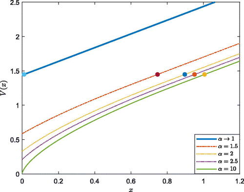
We are mostly concerned with the effects of the ambiguity aversion coefficient $\gamma$ and the transaction cost factor $\alpha .$ Figure 1 illustrates the evolution of the value function under different $\gamma .$ In Figure 2, we present the value function under different $\alpha .$ The x-coordinate of the marked point represents the smooth-pasting boundary of each curve. Figures 1 and 2 show the positive relationship between the value function and initial capital. The value function is a concave function of x. In addition, we observe that when x is larger than the smooth-pasting boundary, the value function is a linear function of x. Figure 1 reveals that when the AAI is more averse to model uncertainty, the value function becomes small. When the AAI is ambiguity neutral––that is, $\gamma =0$––the value function is the largest. In addition, when $\alpha$ increases, the cost of equity issuance increases, and the AAI has a smaller value function, which is depicted in Figure 2. Figure 2 also shows that when there is no transaction cost ($\alpha =1$), the value function increases linearly with the initial capital.

FIGURE 1. Effect of $\gamma$ on $V(x).$

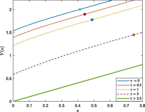
FIGURE 2. Effect of $\alpha$ on $V(x).$

6.2. Smooth-Pasting Boundary $x^{*}$

We are also interested in the effects of transaction costs and ambiguity attitude on the smooth-pasting boundary. In Figure 3 we show the curve of smooth-pasting boundary for $\alpha$ under different $\gamma .$ When $\alpha \to 1,$ the smooth-pasting boundary will converge rapidly to 0. When there is no cost of equity issuance, the insurer can be financed at any time to avoid bankruptcy. Thus, there is no need to hold the reserves. 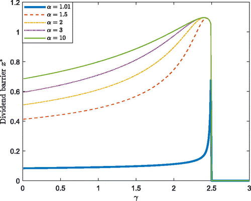In Figure 4 we show the curve of smooth-pasting boundary for $\gamma$ under different $\alpha .$ Figures 3 and 4 show the positive relationship between the smooth-pasting boundary and the transaction costs. When the cost of equity issuance increases, the AAI becomes conservative when paying out dividends. In Figure 4, we see that the smooth-pasting boundary increases with $\gamma$ first and then decreases to zero. When the risk aversion coefficient $\gamma$ becomes larger, the AAI should increase its smooth-pasting boundary to avoid premature bankruptcy in the worst case. However, when $\gamma$ is large enough, paying out all of the dividends and obtaining the deterministic bonus is the optimal choice. Using (5.5)(5.5) $$x_1=k\left(\frac{\mu }{2\delta }-C_2\right),x_2=x_1+\frac{1}{(u_1-u_2)(\gamma -1)}\mathrm{\text{ln}}\hspace{0.17em}\frac{(\frac{2\delta }{\mu }-u_2)(w_2-u_1)}{(\frac{2\delta }{\mu }-u_1)(w_2-u_2)},$$(5.5) , we can obtain that when $\gamma$ tends toward $\frac{{\mu }^2}{2\delta {\sigma }^2}=2.5$ from the left side, the smooth-pasting boundary will converge to $\frac{\mu }{2\delta }=1,$ and Case 3 indicates that for $\gamma ⩾2.5,$ the smooth-pasting boundary always equals 0. In addition, we can observe that the smooth-pasting boundary has a positive relationship with $\gamma$ in most cases. However, when $\gamma$ approaches $\frac{{\mu }^2}{2\delta {\sigma }^2},$ a negative relationship is observed in Figure 4.

FIGURE 3. Effect of $\gamma$ on $x^{*}.$

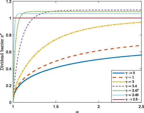
FIGURE 4. Effect of $\alpha$ on $x^{*}.$

6.3. Reinsurance Strategy

Figures 5 and 6 illustrate the effect of $\gamma$ on the robust reinsurance strategy. When $\gamma$ is higher than $\frac{{\mu }^2}{2\delta {\sigma }^2}=2.5,$ the AAI goes bankrupt immediately and takes no insurance risk, which belongs to Case 3 in Section 5. When $\gamma <2.5$ and $\gamma \ne 1,$ the robust strategies follow Case 1 in Section 5. Further, $\gamma =1$ shows the results of Case 2 in Section 5. In Figures 5 and 6, we observe that when the AAI has a higher ambiguity aversion attitude, it becomes more conservative and takes less insurance risk by itself. Furthermore, the reinsurance strategy increases linearly with x first and then remains at 1 in Case 1 and Case 2. The AAI diversifies all of the insurance risk in Case 3, which is shown in Figures 5 and 6. We also note that when $\gamma =0,$ in the case with a small cost $\alpha =1.5,$ the AAI always takes the whole insurance risk by itself, which belongs to situation 2 of Case 1. When $\gamma =0$ and $\alpha =3,$ the solution belongs to situation 1 of Case 1. When the cost of equity issuance increases, the AAI diversifies part of the insurance risk to avoid the large financing cost. 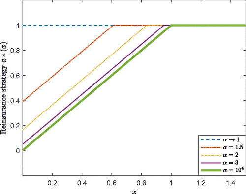As such, there is a difference in Figures 5 and 6 with different $\alpha .$ Briefly, the reinsurance policy is more conservative when the financing cost is larger. The effect of $\alpha$ on the robust reinsurance strategy is plotted in Figure 7. When $\alpha$ increases, the cost of equity issuance is more expensive. Then the AAI has less available surplus and will take smaller insurance risks by itself. When $\alpha$ approaches 1, the reinsurance strategy is 1 and the AAI does not purchase the proportional reinsurance. Interestingly, no matter how large the financing cost is, the AAI will undertake all of the insurance risk when the reserves are large enough.

FIGURE 5. Effect of $\gamma$ on the Robust Reinsurance Strategy When $\alpha =1.5.$

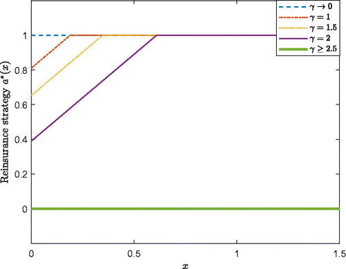
FIGURE 6. Effect of $\gamma$ on the Robust Reinsurance Strategy When $\alpha =3.$

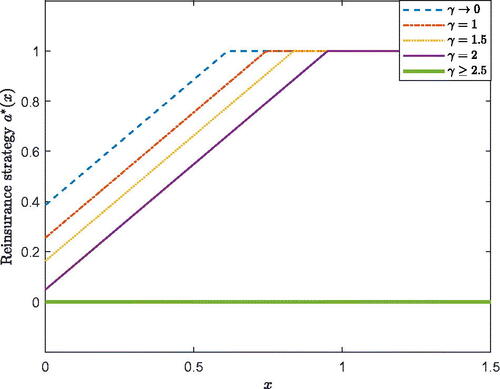
FIGURE 7. Effect of $\alpha$ on the Robust Reinsurance Strategy.

7. CONCLUSION

In this article, we study the robust optimal triple control on dividend, financing, and reinsurance for an AAI. The reserves process is modeled by a drifted Brownian motion. The AAI is ambiguous about the drift term of the reserves process and searches the robust strategies, which are formulated by the max–min optimization problem. The AAI aims to maximize the expected discounted dividend payments minus the expected discounted costs of issuing new equity before bankruptcy under the worst-case scenario. The verification theorem of the robust singular-regular optimization problem is shown and proved in our work. We see that different from He and Liang (2008), ambiguity aversion leads to a nonlinear form in the verification theorem, which causes great difficulties. Based on the verification theorem, three cases of results are obtained, corresponding to small ambiguity aversion, specific ambiguity aversion, and high ambiguity aversion.

As far as we know, the combination of model uncertainty and financing policy has not been studied yet. In the first two cases, equity issuance reflects the reserves process at 0 and prevents the bankruptcy of the AAI. In addition, the cost of the equity issuance and ambiguity attitude make the robust reinsurance and dividend strategies more conservative. The negative effects of transaction costs and ambiguity attitude on the value function are also presented in the numerical results.

ACKNOWLEDGMENTS

The authors are grateful to the members of the group of Actuarial Science and Mathematical Finance in the Department of Mathematical Sciences, Tsinghua University for their feedback and useful conversations.

Additional information

Funding

The authors acknowledge support from the National Natural Science Foundation of China (Grant Nos. 11901574, 12271290, 11871036), the MOE Project of Key Research Institute of Humanities and Social Sciences (22JJD910003), and the National Social Science Fund of China (20AZD075). YL gratefully acknowledges financial support from the research startup fund at The Chinese University of Hong Kong, Shenzhen.

Notes

1 Chakraborty, Cohen, and Young (2021) proved the uniqueness of the solution in the optimal dividends problem under model uncertainty. The penalty term in Chakraborty, Cohen, and Young (2021) does not contain the value function, and the explicit solution is not derived. In our work, to obtain an explicit solution, we add the value function in the penalty term and the uniqueness is not proved. As such, we call the dividend barrier the smooth-pasting boundary instead.

APPENDIX A.

PROOF OF THEOREM 2

To prove Theorem 2, we first show ${\lambda }_1\in (0,1),$ and then we verify that $V(x)$ satisfies Conditions 1 to 4 in Theorem 1.

Lemma 2.

Under the conditions of Theorem 2, we have ${\lambda }_1\in (0,1).$

Proof of Lemma 2.

Recalling the definition (5.3)(5.3) $${\lambda }_1=\frac{\mu w_2}{2\delta }{\left(\frac{w_2-u_1}{\frac{2\delta }{\mu }-u_1}\right)}^{\frac{u_1}{(u_1-u_2)(\gamma -1)}}{\left(\frac{\frac{2\delta }{\mu }-u_2}{w_2-u_2}\right)}^{\frac{u_2}{(u_1-u_2)(\gamma -1)}}.$$(5.3) of ${\lambda }_1,$ it is equivalent to show $$m_1\hspace{0.17em}\mathrm{\text{ln}}\hspace{0.17em}|w_2-u_1|-m_2\hspace{0.17em}\mathrm{\text{ln}}\hspace{0.17em}|w_2-u_2|+\hspace{0.17em}\mathrm{\text{ln}}\hspace{0.17em}{w}_2<m_1\hspace{0.17em}\mathrm{\text{ln}}\hspace{0.17em}\left|\frac{2\delta }{\mu }-u_1\right|-m_2\hspace{0.17em}\mathrm{\text{ln}}\hspace{0.17em}\left|\frac{2\delta }{\mu }-u_2\right|+\hspace{0.17em}\mathrm{\text{ln}}\hspace{0.17em}\frac{2\delta }{\mu },$$ where $m_1=\frac{u_1}{(u_1-u_2)(\gamma -1)},m_2=\frac{u_2}{(u_1-u_2)(\gamma -1)}.$ Define $f(x)=m_1\hspace{0.17em}\mathrm{\text{ln}}\hspace{0.17em}|x-u_1|-m_2\hspace{0.17em}\mathrm{\text{ln}}\hspace{0.17em}|x-u_2|+\hspace{0.17em}\mathrm{\text{ln}}\hspace{0.17em}x;$ it suffices to prove $f(w_2)<f\left(\frac{2\delta }{\mu }\right).$ Using Lemma 1, we know that both $u_1$ and $u_2$ do not belong to the interval $[w_2,\hspace{0.17em}\frac{2\delta }{\mu }],$ and we have, for $x\in (w_2,\hspace{0.17em}\frac{2\delta }{\mu }],$ $$f^{\prime }(x)=\frac{1}{(u_1-u_2)(\gamma -1)}\left(\frac{u_1}{x-u_1}-\frac{u_2}{x-u_2}\right)+\frac{1}{x}=\frac{\gamma (x-w_1)(x-w_2)}{(\gamma -1)x(x-u_1)(x-u_2)}>0.$$

Therefore, we obtain $f(w_2)<f\left(\frac{2\delta }{\mu }\right).$ ▪

In the following, we prove the two parts of Theorem 2.

Proof of Theorem 2:

when $\alpha >\frac{1}{{\lambda }_1}.$

In this case, we have $C_2<\frac{\mu }{2\delta },$ and hence $x_1>0.$ In addition, Lemma 1 and (5.5)(5.5) $$x_1=k\left(\frac{\mu }{2\delta }-C_2\right),x_2=x_1+\frac{1}{(u_1-u_2)(\gamma -1)}\mathrm{\text{ln}}\hspace{0.17em}\frac{(\frac{2\delta }{\mu }-u_2)(w_2-u_1)}{(\frac{2\delta }{\mu }-u_1)(w_2-u_2)},$$(5.5) show that $x_2>x_1.$ Therefore, $V(x)$ in Theorem 2 is well-defined. We note that $$w(x)={\int }_{x_1}^x\left(\frac{u_2-u_1}{C_4{e}^{(u_1-u_2)(\gamma -1)t}-1}+u_2\right)\mathrm{d}t={\int }_{x_1}^x\mathrm{d}\left(u_{1}t+\frac{1}{1-\gamma }\mathrm{\text{ln}}\hspace{0.17em}\left|C_4{e}^{(u_1-u_2)(\gamma -1)t}-1\right|\right);$$ thus, (5.9)(5.9) $$V(x)=C_3{e}^{u_1(x-x_1)}{\left(\frac{C_4{e}^{(u_1-u_2)(\gamma -1)x}-1}{C_4{e}^{(u_1-u_2)(\gamma -1)x_1}-1}\right)}^{\frac{1}{1-\gamma }}.$$(5.9) holds. Moreover, one can verify that $u(x)$ defined in (5.8)(5.8) $$u(t)=\frac{V^{\prime }(t)}{V(t)}\triangleq \frac{u_2-u_1}{C_4{e}^{(u_1-u_2)(\gamma -1)t}-1}+u_2,$$(5.8) satisfies the following ordinary differential equation (ODE): (A.1) $$u^{\prime }(x)=(\gamma -1)u{(x)}^2-\frac{2\mu }{{\sigma }^2}u(x)+\frac{2\delta }{{\sigma }^2}.$$(A.1)

In this light, for $x\in (x_1,x_2],$ we have (A.2) $$\begin{array}{c}{V}^{″}(x)=V(x)\left(u^{\prime }(x)+u{(x)}^2\right)=V(x)\left[\gamma u{(x)}^2-\frac{2\mu }{{\sigma }^2}u(x)+\frac{2\delta }{{\sigma }^2}\right].\hfill \end{array}$$(A.2)

Recalling the definition of $C_4,$ $x_1,$ and $x_2$ in (5.5)(5.5) $$x_1=k\left(\frac{\mu }{2\delta }-C_2\right),x_2=x_1+\frac{1}{(u_1-u_2)(\gamma -1)}\mathrm{\text{ln}}\hspace{0.17em}\frac{(\frac{2\delta }{\mu }-u_2)(w_2-u_1)}{(\frac{2\delta }{\mu }-u_1)(w_2-u_2)},$$(5.5) and (5.6)(5.6) $$C_1=\alpha C_2^{1-k},C_3=C_1{\left(\frac{\mu }{2\delta }\right)}^k,C_4=\frac{\frac{2\delta }{\mu }-u_1}{\frac{2\delta }{\mu }-u_2}{e}^{-(u_1-u_2)(\gamma -1)x_1}.$$(5.6) , we have (A.3) $$C_4{e}^{(u_1-u_2)(\gamma -1)x_1}=\frac{\frac{2\delta }{\mu }-u_1}{\frac{2\delta }{\mu }-u_2}$$(A.3) and (A.4) $$C_4{e}^{(u_1-u_2)(\gamma -1)x_2}=\frac{\frac{2\delta }{\mu }-u_1}{\frac{2\delta }{\mu }-u_2}{e}^{(u_1-u_2)(\gamma -1)(x_2-x_1)}=\frac{w_2-u_1}{w_2-u_2},$$(A.4) which leads to (A.5) $$u(x_1)=\frac{2\delta }{\mu },u(x_2)=w_2.$$(A.5)

Based on the calculation above, we use the following Steps 1 to 4 to prove the theorem:

• Step 1. We verify that Condition 1 in Theorem 1 holds; that is, $V\in C^2[0,+\infty ),$ which is equivalent to show for $x\in \{x_1,x_2\}:$ $$V(x-)=V(x+),V^{\prime }(x-)=V^{\prime }(x+),V^{″}(x-)=V^{″}(x+).$$

(1.a) For $x=x_1,$ we have from (5.7)(5.7) $$V(x)=\{\begin{array}{lll}{C}_1{\left(\frac{1}{k}x+C_2\right)}^k,\hfill & \hfill & 0⩽x⩽x_1,\hfill \\ C_3{e}^{w(x)},\hfill & \hfill & x_1<x⩽x_2,\hfill \\ V(x_2)+x-x_2,\hfill & \hfill & x>x_2,\hfill \end{array}$$(5.7) and (A.2)(A.2) $$\begin{array}{c}{V}^{″}(x)=V(x)\left(u^{\prime }(x)+u{(x)}^2\right)=V(x)\left[\gamma u{(x)}^2-\frac{2\mu }{{\sigma }^2}u(x)+\frac{2\delta }{{\sigma }^2}\right].\hfill \end{array}$$(A.2) that $$\{\begin{array}{l}V(x_1-)=C_1{\left(\frac{x_1}{k}+C_2\right)}^k=C_1{\left(\frac{\mu }{2\delta }\right)}^k,?V(x_1+)=C_3{e}^{w(x_1)}=C_3=V(x_1-);\hfill \\ V^{\prime }(x_1-)=C_1{\left(\frac{\mu }{2\delta }\right)}^{k-1},V^{\prime }(x_1+)=C_3{e}^{w(x_1)}u(x_1)=\frac{2\delta }{\mu }{C}_3=V^{\prime }(x_1-);\hfill \\ V^{″}(x_1-)=\frac{k-1}{k}{C}_1{\left(\frac{\mu }{2\delta }\right)}^{k-2}=\frac{k-1}{k}\frac{4{\delta }^2}{{\mu }^2}V(x_1-)=V(x_1+)\left(\frac{4\gamma {\delta }^2}{{\mu }^2}-\frac{2\delta }{{\sigma }^2}\right);\hfill \\ V^{″}(x_1+)=V(x_1+)\left[\gamma u{(x_1)}^2-\frac{2\mu }{{\sigma }^2}u(x_1)+\frac{2\delta }{{\sigma }^2}\right]=V(x_1+)\left(\frac{4\gamma {\delta }^2}{{\mu }^2}-\frac{2\delta }{{\sigma }^2}\right)=V^{″}(x_1-).\hfill \end{array}$$

(1.b) For $x=x_2,$ it is obvious that $V(x_2-)=V(x_2+).$ Recalling that definition of $w_2$ in (5.2)(5.2) $$w_1=\frac{\mu +\sqrt{{\mu }^2-2\delta {\sigma }^2\gamma }}{\gamma {\sigma }^2},w_2=\frac{\mu -\sqrt{{\mu }^2-2\delta {\sigma }^2\gamma }}{\gamma {\sigma }^2}.$$(5.2) , we have $$V^{″}(x_2-)=V(x_2-)\left(\gamma w_2^2-\frac{2\mu }{{\sigma }^2}{w}_2+\frac{2\delta }{{\sigma }^2}\right)=0=V^{″}(x_2+),$$ and it remains to show $V^{\prime }(x_2-)=1=V^{\prime }(x_2+).$ In fact, using (5.9)(5.9) $$V(x)=C_3{e}^{u_1(x-x_1)}{\left(\frac{C_4{e}^{(u_1-u_2)(\gamma -1)x}-1}{C_4{e}^{(u_1-u_2)(\gamma -1)x_1}-1}\right)}^{\frac{1}{1-\gamma }}.$$(5.9) , (A.3)(A.3) $$C_4{e}^{(u_1-u_2)(\gamma -1)x_1}=\frac{\frac{2\delta }{\mu }-u_1}{\frac{2\delta }{\mu }-u_2}$$(A.3) , and (A.4)(A.4) $$C_4{e}^{(u_1-u_2)(\gamma -1)x_2}=\frac{\frac{2\delta }{\mu }-u_1}{\frac{2\delta }{\mu }-u_2}{e}^{(u_1-u_2)(\gamma -1)(x_2-x_1)}=\frac{w_2-u_1}{w_2-u_2},$$(A.4) , we have $$\begin{array}{cc}{V}^{\prime }(x_2-)\hfill & =V(x_2)u(x_2)\hfill \\ \hfill & =w_2{C}_3{e}^{u_1(x_2-x_1)}{\left(\frac{C_4{e}^{(u_1-u_2)(\gamma -1)x_2}-1}{C_4{e}^{(u_1-u_2)(\gamma -1)x_1}-1}\right)}^{\frac{1}{1-\gamma }}\hfill \\ \hfill & =w_2{C}_1{\left(\frac{\mu }{2\delta }\right)}^k{\left(\frac{(\frac{2\delta }{\mu }-u_2)(w_2-u_1)}{(\frac{2\delta }{\mu }-u_1)(w_2-u_2)}\right)}^{\frac{u_1}{(u_1-u_2)(\gamma -1)}}{\left(\frac{\frac{2\delta }{\mu }-u_2}{w_2-u_2}\right)}^{\frac{1}{1-\gamma }}\hfill \\ \hfill & =\alpha w_2{C}_2^{1-k}{\left(\frac{\mu }{2\delta }\right)}^k{\left(\frac{w_2-u_1}{\frac{2\delta }{\mu }-u_1}\right)}^{\frac{u_1}{(u_1-u_2)(\gamma -1)}}{\left(\frac{\frac{2\delta }{\mu }-u_2}{w_2-u_2}\right)}^{\frac{u_2}{(u_1-u_2)(\gamma -1)}}\hfill \\ \hfill & =1,\hfill \end{array}$$ where the last “=” comes from the definition of $C_2$ in (5.4)(5.4) $$C_2^{k-1}=\alpha {\lambda }_1{\left(\frac{\mu }{2\delta }\right)}^{k-1}.$$(5.4) .

Concluding the results above, we have proved $V\in C^2[0,+\infty ).$

• Step 2. We prove for $x\in [0,x_2]:$ $$\underset{a\in [0,1]}{\mathrm{\text{sup}}}\left[\frac{{\sigma }^2}{2}(V^{″}(x)-\gamma \frac{V^{\prime }{(x)}^2}{V(x)})a^2+\mu V^{\prime }(x)a-\delta V(x)\right]=0.$$

1. For $0⩽x⩽x_1,$ we have $$-\frac{\mu V^{\prime }(x)}{{\sigma }^2\left(V^{″}(x)-\gamma \frac{V^{\prime }{(x)}^2}{V(x)}\right)}=\frac{2\delta }{\mu }\left(\frac{x}{k}+C_2\right)\in [0,1].$$

As such, we know $$\begin{array}{c}\underset{a\in [0,1]}{\text{arg\hspace{0.17em}sup}}\left[\frac{{\sigma }^2}{2}(V^{″}(x)-\gamma \frac{V^{\prime }{(x)}^2}{V(x)})a^2+\mu V^{\prime }(x)a-\delta V(x)\right]\\ =-\frac{\mu V^{\prime }(x)}{{\sigma }^2\left(V^{″}(x)-\gamma \frac{V^{\prime }{(x)}^2}{V(x)}\right)}\\ =\frac{2\delta }{\mu }\left(\frac{x}{k}+C_2\right),\end{array}$$ and hence one can obtain (A.6) $$\begin{array}{cc}\hfill & \underset{a\in [0,1]}{\mathrm{\text{sup}}}\left[\frac{{\sigma }^2}{2}(V^{″}(x)-\gamma \frac{V^{\prime }{(x)}^2}{V(x)})a^2+\mu V^{\prime }(x)a-\delta V(x)\right]=0\hfill \\ \hfill & \iff \frac{{\mu }^2}{2\delta {\sigma }^2}{V}^{\prime }{(x)}^2+V(x)V^{″}(x)-\gamma V^{\prime }{(x)}^2=0.\hfill \end{array}$$(A.6)

This is a homogeneous ODE and can be solved by applying transformation $u(x)=\frac{V^{\prime }(x)}{V(x)},$ which leads to $$\left(\frac{{\mu }^2}{2\delta {\sigma }^2}-\gamma +1\right)u{(x)}^2+u^{\prime }(x)=0.$$

It is easy to verify that $u(x)={(\frac{x}{k}+C_2)}^{-1}$ satisfies the above ODE, and we have proved for $0⩽x⩽x_1$ that $$\underset{a\in [0,1]}{\mathrm{\text{sup}}}\left[\frac{{\sigma }^2}{2}(V^{″}(x)-\gamma \frac{V^{\prime }{(x)}^2}{V(x)})a^2+\mu V^{\prime }(x)a-\delta V(x)\right]=0.$$

• b. For $x_1⩽x⩽x_2,$ we first prove (A.7) $$\frac{{\sigma }^2}{2}\left(V^{″}(x)-\gamma \frac{V^{\prime }{(x)}^2}{V(x)}\right)+\mu V^{\prime }(x)-\delta V(x)=0.$$(A.7)

In fact, applying $u(x)=\frac{V^{\prime }(x)}{V(x)}$ and recalling (5.1)(5.1) $$u_1=\frac{\mu +\sqrt{{\mu }^2-2\delta {\sigma }^2(\gamma -1)}}{(\gamma -1){\sigma }^2},u_2=\frac{\mu -\sqrt{{\mu }^2-2\delta {\sigma }^2(\gamma -1)}}{(\gamma -1){\sigma }^2}.$$(5.1) , the above ODE is equivalent to (A.8) $$u^{\prime }(x)=(\gamma -1)u{(x)}^2-\frac{2\mu }{{\sigma }^2}u(x)+\frac{2\delta }{{\sigma }^2}=(\gamma -1)\left[u(x)-u_1\right]\left[u(x)-u_2\right],$$(A.8) which is exactly (A.1)(A.1) $$u^{\prime }(x)=(\gamma -1)u{(x)}^2-\frac{2\mu }{{\sigma }^2}u(x)+\frac{2\delta }{{\sigma }^2}.$$(A.1) , and hence (A.7)(A.7) $$\frac{{\sigma }^2}{2}\left(V^{″}(x)-\gamma \frac{V^{\prime }{(x)}^2}{V(x)}\right)+\mu V^{\prime }(x)-\delta V(x)=0.$$(A.7) holds. In addition, we can write (A.2)(A.2) $$\begin{array}{c}{V}^{″}(x)=V(x)\left(u^{\prime }(x)+u{(x)}^2\right)=V(x)\left[\gamma u{(x)}^2-\frac{2\mu }{{\sigma }^2}u(x)+\frac{2\delta }{{\sigma }^2}\right].\hfill \end{array}$$(A.2) as follows: (A.9) $$\begin{array}{c}{V}^{″}(x)=\gamma V(x)\left[u(x)-w_1\right]\left[u(x)-w_2\right].\hfill \end{array}$$(A.9)

Using (A.5)(A.5) $$u(x_1)=\frac{2\delta }{\mu },u(x_2)=w_2.$$(A.5) and Lemma 1, when $\gamma >1,$ it holds that $u_1>u(x_1)>u(x_2)>u_2,$ and then (A.8)(A.8) $$u^{\prime }(x)=(\gamma -1)u{(x)}^2-\frac{2\mu }{{\sigma }^2}u(x)+\frac{2\delta }{{\sigma }^2}=(\gamma -1)\left[u(x)-u_1\right]\left[u(x)-u_2\right],$$(A.8) yields $u^{\prime }(x)<0$ on $[x_1,x_2].$ As such, for $x\in [x_1,x_2],$ we have $\frac{\delta }{\mu }<w_2⩽u(x)⩽\frac{2\delta }{\mu }<w_1.$

For $\gamma <1,$ we have $u(x_1)>u(x_2)>\frac{\delta }{\mu }>u_2>u_1,$ which also leads to $u^{\prime }(x)<0$ on $[x_1,x_2].$ In this light, for $x\in [x_1,x_2],$ we still have $\frac{\delta }{\mu }<w_2⩽u(x)⩽\frac{2\delta }{\mu }<w_1.$

To conclude, for $\gamma \cancel{=}1$ and $x\in [x_1,x_2],$ we have (A.10) $$\frac{\delta }{\mu }<w_2⩽u(x)⩽\frac{2\delta }{\mu }<w_1,u^{\prime }(x)<0.$$(A.10)

Based on the discussion above, we have $$-\frac{\mu V^{\prime }(x)}{{\sigma }^2\left(V^{″}(x)-\gamma \frac{V^{\prime }{(x)}^2}{V(x)}\right)}=\frac{1}{2}\frac{\mu V^{\prime }(x)}{\mu V^{\prime }(x)-\delta V(x)}=\frac{1}{2}\frac{u(x)}{u(x)-\frac{\delta }{\mu }}⩾1,$$ and hence, for $x\in [x_1,x_2],$ it holds that $$\underset{a\in [0,1]}{\text{arg\hspace{0.17em}sup}}\left[\frac{{\sigma }^2}{2}(V^{″}(x)-\gamma \frac{V^{\prime }{(x)}^2}{V(x)})a^2+\mu V^{\prime }(x)a-\delta V(x)\right]=1.$$

Therefore, (A.7)(A.7) $$\frac{{\sigma }^2}{2}\left(V^{″}(x)-\gamma \frac{V^{\prime }{(x)}^2}{V(x)}\right)+\mu V^{\prime }(x)-\delta V(x)=0.$$(A.7) shows $$\begin{array}{cc}\underset{a\in [0,1]}{\mathrm{\text{sup}}}\hfill & \left[\frac{{\sigma }^2}{2}(V^{″}(x)-\gamma \frac{V^{\prime }{(x)}^2}{V(x)})a^2+\mu V^{\prime }(x)a-\delta V(x)\right]\hfill \\ \hfill & =\frac{{\sigma }^2}{2}\left(V^{″}(x)-\gamma \frac{V^{\prime }{(x)}^2}{V(x)}\right)+\mu V^{\prime }(x)-\delta V(x)=0.\hfill \end{array}$$

• Step 3. We prove for $x⩾x_2,$ $$\underset{a\in [0,1]}{\mathrm{\text{sup}}}\left[\frac{{\sigma }^2}{2}(V^{″}(x)-\gamma \frac{V^{\prime }{(x)}^2}{V(x)})a^2+\mu V^{\prime }(x)a-\delta V(x)\right]⩽0.$$

In fact, for $x⩾x_2,$ we know that $V^{\prime }(x)=1$ and $V^{″}(x)=0;$ thus, it suffices to verify (A.11) $$\underset{a\in [0,1]}{\mathrm{\text{sup}}}\left[-\frac{\gamma {\sigma }^2}{2V(x)}{a}^2+\mu a-\delta V(x)\right]⩽0.$$(A.11)

As $V(x)⩾V(x_2)=\frac{V^{\prime }(x_2)}{u(x_2)}=\frac{1}{w_2},$ using (5.2)(5.2) $$w_1=\frac{\mu +\sqrt{{\mu }^2-2\delta {\sigma }^2\gamma }}{\gamma {\sigma }^2},w_2=\frac{\mu -\sqrt{{\mu }^2-2\delta {\sigma }^2\gamma }}{\gamma {\sigma }^2}.$$(5.2) , we have $\frac{\mu V(x)}{\gamma {\sigma }^2}⩾\frac{1}{w_2}\frac{\mu }{\gamma {\sigma }^2}>1.$ As such, $$\underset{a\in [0,1]}{\text{arg\hspace{0.17em}sup}}\left[-\frac{\gamma {\sigma }^2}{2V(x)}{a}^2+\mu a-\delta V(x)\right]=1.$$

Therefore, (A.11)(A.11) $$\underset{a\in [0,1]}{\mathrm{\text{sup}}}\left[-\frac{\gamma {\sigma }^2}{2V(x)}{a}^2+\mu a-\delta V(x)\right]⩽0.$$(A.11) is equivalent to (A.12) $$\begin{array}{cc}0\hfill & ⩾-\frac{\gamma {\sigma }^2}{2V(x)}+\mu -\delta V(x)\hfill \\ \hfill & =-\frac{{\sigma }^{2}V(x)}{2}\left[\frac{\gamma }{V{(x)}^2}-\frac{2\mu }{{\sigma }^2}\frac{1}{V(x)}+\frac{2\delta }{{\sigma }^2}\right]\hfill \\ \hfill & =-\frac{{\sigma }^{2}V(x)}{2}\left[\frac{1}{V(x)}-w_1\right]\left[\frac{1}{V(x)}-w_2\right],x⩾x_2.\hfill \end{array}$$(A.12)

As for $x⩾x_2,$ we have $V(x)⩾V(x_2)⩾\frac{1}{w_2}>\frac{1}{w_1};$ thus, (A.12)(A.12) $$\begin{array}{cc}0\hfill & ⩾-\frac{\gamma {\sigma }^2}{2V(x)}+\mu -\delta V(x)\hfill \\ \hfill & =-\frac{{\sigma }^{2}V(x)}{2}\left[\frac{\gamma }{V{(x)}^2}-\frac{2\mu }{{\sigma }^2}\frac{1}{V(x)}+\frac{2\delta }{{\sigma }^2}\right]\hfill \\ \hfill & =-\frac{{\sigma }^{2}V(x)}{2}\left[\frac{1}{V(x)}-w_1\right]\left[\frac{1}{V(x)}-w_2\right],x⩾x_2.\hfill \end{array}$$(A.12) holds.

• Step 4. We verify Conditions 2, 3, and 4 in Theorem 1.

Using (A.9)(A.9) $$\begin{array}{c}{V}^{″}(x)=\gamma V(x)\left[u(x)-w_1\right]\left[u(x)-w_2\right].\hfill \end{array}$$(A.9) and (A.10)(A.10) $$\frac{\delta }{\mu }<w_2⩽u(x)⩽\frac{2\delta }{\mu }<w_1,u^{\prime }(x)<0.$$(A.10) , we know that $V^{″}(x)<0$ on $[x_1,x_2)$ and $V^{″}(x_2)=0.$ In addition, as in Case 1, we have $k<1,$ (5.7)(5.7) $$V(x)=\{\begin{array}{lll}{C}_1{\left(\frac{1}{k}x+C_2\right)}^k,\hfill & \hfill & 0⩽x⩽x_1,\hfill \\ C_3{e}^{w(x)},\hfill & \hfill & x_1<x⩽x_2,\hfill \\ V(x_2)+x-x_2,\hfill & \hfill & x>x_2,\hfill \end{array}$$(5.7) indicates that $V^{″}(x)<0$ also holds on $[0,x_1].$ As $V^{\prime }(x)=1$ for $x⩾x_2$ and $V^{\prime }(0)=C_1{C}_2^{k-1}=\alpha ,$ we obtain Condition 2 by taking $x^{*}=x_2.$

As for Condition 3, the results of Step 2 and Step 3 indicate that for $x\in [0,x_2],$ we have $$\underset{a\in [0,1]}{\mathrm{\text{sup}}}\left[\frac{{\sigma }^2}{2}(V^{″}(x)-\gamma \frac{V^{\prime }{(x)}^2}{V(x)})a^2+\mu V^{\prime }(x)a-\delta V(x)\right]=0,V^{\prime }(x)\in [1,\alpha ],$$ and for $x⩾x_2,$ we have $$\underset{a\in [0,1]}{\mathrm{\text{sup}}}\left[\frac{{\sigma }^2}{2}(V^{″}(x)-\gamma \frac{V^{\prime }{(x)}^2}{V(x)})a^2+\mu V^{\prime }(x)a-\delta V(x)\right]⩽0,V^{\prime }(x)-\alpha <0=V^{\prime }(x)-1.$$

Therefore, Condition 3 is also satisfied by V.

Finally, for Condition 4, we have from Step 2 that $$a^{*}(x)=\{\begin{array}{ccc}\frac{2\delta }{\mu }\left(\frac{x}{k}+C_2\right),\hfill & \hfill & 0⩽x⩽x_1,\hfill \\ 1,\hfill & \hfill & x_1⩽x⩽x_2,\hfill \end{array}$$ which is obviously a Lipschitz function. ▪

Proof of Theorem 2:

when $\alpha ⩽\frac{1}{{\lambda }_1}.$

Consider the following equation: $$g(x)\triangleq \alpha w_2{e}^{u_{1}x}{\left|\frac{1}{C_6(x)-1}\frac{u_2-u_1}{w_2-u_2}\right|}^{\frac{1}{1-\gamma }}\left|\frac{C_6(x)-1}{u_2{C}_6(x)-u_1}\right|=1.$$

Recalling that $C_6(x)=\frac{w_2-u_1}{w_2-u_2}{e}^{-(u_1-u_2)(\gamma -1)x},$ using Lemma 1, there exists $x_3^{*}>0$ such that $$e^{(u_1-u_2)(\gamma -1)x_3^{*}}=\frac{w_2-u_1}{\frac{2\delta }{\mu }-u_1}\frac{\frac{2\delta }{\mu }-u_2}{w_2-u_2}>1,$$ and we have $$C_6(x_3^{*})=\frac{\frac{2\delta }{\mu }-u_1}{\frac{2\delta }{\mu }-u_2},g(x_3^{*})=\alpha {\lambda }_1⩽1,g(0)=\alpha >1.$$

In addition, for $x\in [0,x_3^{*}],$ if $\gamma >1,$ then $C_6(x)<0<u_2<u_1$ and hence $u_2{C}_6(x)-u_1<0,$ which means that g is continuous. If $\gamma <1,$ then $C_6(x)⩾C_6(x_3^{*})>1$ and $u_2>0>u_1,$ and hence $u_2{C}_6(x)-u_1>0,$ which also implies that g is continuous.

Therefore, the intermediate value theorem tells that there exists $x_3\in (0,x_3^{*}]$ such that $g(x_3)=1.$ Noting that similar to the case when $\alpha >\frac{1}{\lambda },$ we have, for $x\in [0,x_3],$ $$v(x)\triangleq \frac{V^{\prime }(x)}{V(x)}=\frac{u_2-u_1}{C_6(x_3)e^{(u_1-u_2)(\gamma -1)x}-1}+u_2$$ and $$V^{″}(x)=\gamma V(x)\left[v(x)-w_1\right]\left[v(x)-w_2\right].$$

For this $x_3,$ recalling $C_5(x_3)=\frac{1}{w_2}{e}^{-u_1{x}_3}{(\frac{u_2-u_1}{u_2-w_2})}^{\frac{1}{\gamma -1}},$ we have $$V^{\prime }(0)=V(0)\frac{u_2{C}_6(x_3)-u_1}{C_6(x_3)-1}=C_5(x_3){\left|C_6(x_3)-1\right|}^{\frac{1}{1-\gamma }}\frac{u_2{C}_6(x_3)-u_1}{C_6(x_3)-1}=\frac{\alpha }{g(x_3)}=\alpha .$$

In addition, as $C_6(x_3)e^{(u_1-u_2)(\gamma -1)x_3}=\frac{w_2-u_1}{w_2-u_2},$ we know that $v(x_3)=w_2,$ $V^{″}(x_3)=0,$ and $$V^{\prime }(x_3)=V(x_3)v(x_3)=C_5(x_3)w_2{e}^{u_1{x}_3}{\left|\frac{u_2-u_1}{w_2-u_2}\right|}^{\frac{1}{1-\gamma }}=1.$$

Based on the discussion above, one can verify that V satisfies Conditions 1 to 4 in Theorem 1 by the same steps as in the proof of the first part. ▪

APPENDIX B.

PROOF OF THEOREM 4

Proof of Theorem 4.

On the one hand, if we take ${\pi }^{*}=(a^{*},L^{*},G^{*})$ by $a_s^{*}\equiv G_s^{*}\equiv 0$ and $L_s^{*}\equiv x,$ then $X_s^{*}\equiv 0,$ and for $\varphi \in \Phi ,$ we have $J_V({\pi }^{*},\varphi )={\mathbb{E}}^{{\mathbb{Q}}^{\varphi }}\left[L_0\right]=x,$ which yields $$\underset{\pi \in \Pi (x)}{\mathrm{\text{sup}}}\underset{\varphi \in \Phi }{\mathrm{\text{inf}}}{J}_V(\pi ,\varphi )⩾\underset{\varphi \in \Phi }{\mathrm{\text{inf}}}{J}_V({\pi }^{*},\varphi )=x.$$

On the other hand, for $V(x)=x,$ it is easy to verify that Conditions 1 and 2 in Theorem 1 hold for $x>0.$ Following the proof of Theorem 1, we obtain $V(x)⩾\underset{\pi \in \Pi (x)}{\mathrm{\text{sup}}}\underset{\varphi \in \Phi }{\mathrm{\text{inf}}}{J}_V(\pi ,\varphi ).$ Therefore, we have $V(x)=\underset{\pi \in \Pi (x)}{\mathrm{\text{sup}}}\underset{\varphi \in \Phi }{\mathrm{\text{inf}}}{J}_V(\pi ,\varphi ),$ with ${\pi }^{*}$ defined above being the optimal control. ▪

References

- Baltas, I., A. Xepapadeas, and A. N. Yannacopoulos. 2018. Robust portfolio decisions for financial institutions. Journal of Dynamics and Games 5 (2):61. doi:10.3934/jdg.2018006
- Bäuerle, N., and G. Leimcke. 2021. Robust optimal investment and reinsurance problems with learning. Scandinavian Actuarial Journal 2021 (2):82–109. doi:10.1080/03461238.2020.1806917
- Bayraktar, E., A. Cosso, and H. Pham. 2016. Robust feedback switching control: Dynamic programming and viscosity solutions. SIAM Journal on Control and Optimization 54 (5):2594–628. doi:10.1137/15M1046903
- Blanchard, O. J., R. Shiller, and J. J. Siegel. 1993. Movements in the equity premium. Brookings Papers on Economic Activity 1993 (2):75–138. doi:10.2307/2534565
- Branger, N., L. S. Larsen, and C. Munk. 2013. Robust portfolio choice with ambiguity and learning about return predictability. Journal of Banking and Finance 37 (5):1397–411. doi:10.1016/j.jbankfin.2012.05.009
- Chakraborty, P., A. Cohen, and V. R. Young. 2021. Optimal dividends under model uncertainty. arXiv preprint arXiv:2109.09137.
- Chen, Z., and P. Yang. 2020. Robust optimal reinsurance-investment strategy with price jumps and correlated claims. Insurance: Mathematics and Economics 92:27–46. doi:10.1016/j.insmatheco.2020.03.001
- Dai, H., Z. Liu, and N. Luan. 2010. Optimal dividend strategies in a dual model with capital injections. Mathematical Methods of Operations Research 72 (1):129–43. doi:10.1007/s00186-010-0312-7
- Dickson, D. C. M., and H. R. Waters. 2004. Some optimal dividends problems. ASTIN Bulletin 34:49–74. doi:10.2143/AST.34.1.504954
- Ellsberg, D. 1961. Risk, ambiguity, and the Savage axioms. The Quarterly Journal of Economics 75 (4):643–69. doi:10.2307/1884324
- Feng, Y., J. Zhu, and T. K. Siu. 2021. Optimal risk exposure and dividend payout policies under model uncertainty. Insurance: Mathematics and Economics 100:1–29. doi:10.1016/j.insmatheco.2021.03.029
- Gerber, H. U. 1972. Games of economic survival with discrete and continuous income processes. Operations Research 20:37–45. doi:10.1287/opre.20.1.37
- Gerber, H. U., and E. S. Shiu. 2006. On optimal dividend strategies in the compound Poisson model. North American Actuarial Journal 10 (2):76–93. doi:10.1080/10920277.2006.10596249
- Gilboa, I., and D. Schmeidler. 1989. Maxmin expected utility with non-unique prior. Journal of Mathematical Economics 18:141–53. doi:10.1016/0304-4068(89)90018-9
- Guan, G., and Z. Liang. 2019. Robust optimal reinsurance and investment strategies for an AAI with multiple risks. Insurance: Mathematics and Economics 89:63–78. doi:10.1016/j.insmatheco.2019.09.004
- Hansen, L. P., and T. J. Sargent. 2001. Robust control and model uncertainty. American Economic Review 91 (2):60–66. doi:10.1257/aer.91.2.60
- Hansen, L. P., T. J. Sargent, G. Turmuhambetova, and N. Williams. 2006. Robust control and model misspecification. Journal of Economic Theory 128:45–90. doi:10.1016/j.jet.2004.12.006
- He, L., and Z. Liang. 2008. Optimal financing and dividend control of the insurance company with proportional reinsurance policy. Insurance: Mathematics and Economics 42:976–83. doi:10.1016/j.insmatheco.2007.11.003
- He, L., and Z. Liang. 2009. Optimal financing and dividend control of the insurance company with fixed and proportional transaction costs. Insurance: Mathematics and Economics 44:88–94. doi:10.1016/j.insmatheco.2008.10.001
- Jørgensen, B., and M. C. Paes de Souza. 1994. Fitting Tweedie’s compound Poisson model to insurance claims data. Scandinavian Actuarial Journal 1994 (1):69–93. doi:10.1080/03461238.1994.10413930
- Li, D., Y. Zeng, and H. Yang. 2018. Robust optimal excess-of-loss reinsurance and investment strategy for an insurer in a model with jumps. Scandinavian Actuarial Journal 2018 (2):145–71. doi:10.1080/03461238.2017.1309679
- Liang, Z., and M. Ma. 2020. Robust consumption‐investment problem under CRRA and CARA utilities with time‐varying confidence sets. Mathematical Finance 30 (3):1035–72. doi:10.1111/mafi.12217
- Lions, P.-L., and A. S. Sznitman. 1984. Stochastic differential equations with reflecting boundary conditions. Communications on Pure and Applied Mathematics 37:511–37. doi:10.1002/cpa.3160370408
- Liu, W., and Y. Hu. 2014. Optimal financing and dividend control of the insurance company with excess-of-loss reinsurance policy. Statistics and Probability Letters 84:121–30. doi:10.1016/j.spl.2013.09.034
- Løkka, A., and M. Zervos. 2008. Optimal dividend and issuance of equity policies in the presence of proportional costs. Insurance: Mathematics and Economics 42 (3):954–61. doi:10.1016/j.insmatheco.2007.10.013
- Luo, P., and Y. Tian. 2022. Investment, payout, and cash management under risk and ambiguity. Journal of Banking and Finance 141:106551. doi:10.1016/j.jbankfin.2022.106551
- Maenhout, P. J. 2004. Robust portfolio rules and asset pricing. The Review of Financial Studies 17:951–83. doi:10.1093/rfs/hhh003
- Mataramvura, S., and B. Øksendal. 2008. Risk minimizing portfolios and HJBI equations for stochastic differential games. Stochastics 80 (4):317–37. doi:10.1080/17442500701655408
- Meng, H., and T. K. Siu. 2011. Optimal mixed impulse-equity insurance control problem with reinsurance. SIAM Journal on Control and Optimization 49 (1):254–79. doi:10.1137/090773167
- Meraou, M. A., N. M. AI-Kandari, M. Z. Raqab, and D. Kundu. 2022. Analysis of skewed data by using compound Poisson exponential distribution with applications to insurance claims. Journal of Statistical Computation and Simulation 92 (5):928–56. doi:10.1080/00949655.2021.1981324
- Merton, R. C. 1980. On estimating the expected return on the market: An exploratory investigation. Journal of Financial Economics 8 (4):323–61. doi:10.1016/0304-405X(80)90007-0
- Perninge, M. 2021. Finite horizon robust impulse control in a non-Markovian framework and related systems of reflected BSDEs. arXiv preprint arXiv:2103.16272.
- Pu, J., and Q. Zhang. 2021. Robust consumption portfolio optimization with stochastic differential utility. Automatica 133:109835. doi:10.1016/j.automatica.2021.109835
- Pun, C. S. 2021. Robust classical-impulse stochastic control problems in an infinite horizon. doi:http://dx.doi.org/10.2139/ssrn.3925923.
- Schied, A. 2008. Robust optimal control for a consumption-investment problem. Mathematical Methods of Operations Research 67 (1):1–20. doi:10.1007/s00186-007-0172-y
- Sethi, S. P., and M. I. Taksar. 2002. Optimal financing of a corporation subject to random returns. Mathematical Finance 12 (2):155–72. doi:10.1111/1467-9965.t01-2-02002
- Yao, D., H. Yang, and R. Wang. 2010. Optimal financing and dividend strategies in a dual model with proportional costs. Journal of Industrial and Management Optimization 6 (4):761. doi:10.3934/jimo.2010.6.761
- Yi, B., Z. Li, F. G. Viens, and Y. Zeng. 2013. Robust optimal control for an insurer with reinsurance and investment under Heston’s stochastic volatility model. Insurance: Mathematics and Economics 53 (3):601–14. doi:10.1016/j.insmatheco.2013.08.011
- Yin, C., and Y. Wen. 2013. Optimal dividend problem with a terminal value for spectrally positive Lèvy processes. Insurance: Mathematics and Economics 53 (3):769–73. doi:10.1016/j.insmatheco.2013.09.019
- Yin, C., Y. Wen, and Y. Zhao. 2014. On the optimal dividend problem for a spectrally positive Lèvy process. ASTIN Bulletin 44 (3):635–51. doi:10.1017/asb.2014.12
- Yip, K. C., and K. K. Yau. 2005. On modeling claim frequency data in general insurance with extra zeros. Insurance: Mathematics and Economics 36 (2):153–63. doi:10.1016/j.insmatheco.2004.11.002
- Zhang, X., and T. K. Siu. 2009. Optimal investment and reinsurance of an insurer with model uncertainty. Insurance: Mathematics and Economics 45 (1):81–88. doi:10.1016/j.insmatheco.2009.04.001
- Zhu, J. 2017. Optimal financing and dividend distribution with transaction costs in the case of restricted dividend rates. ASTIN Bulletin 47 (1):239–68. doi:10.1017/asb.2016.29
- Zou, Z. 2020. Optimal dividend-distribution strategy under ambiguity aversion. Operations Research Letters 48 (4):435–40. doi:10.1016/j.orl.2020.05.004