Antidiscrimination Insurance Pricing: Regulations, Fairness Criteria, and Models

Abstract

On the issue of insurance discrimination, a grey area in regulation has resulted from the growing use of big data analytics by insurance companies: direct discrimination is prohibited, but indirect discrimination using proxies or more complex and opaque algorithms is not clearly specified or assessed. This phenomenon has recently attracted the attention of insurance regulators all over the world. Meanwhile, various fairness criteria have been proposed and flourished in the machine learning literature with the rapid growth of artificial intelligence (AI) in the past decade and have mostly focused on classification decisions. In this article, we introduce some fairness criteria that are potentially applicable to insurance pricing as a regression problem to the actuarial field, match them with different levels of potential and existing antidiscrimination regulations, and implement them into a series of existing and newly proposed antidiscrimination insurance pricing models, using both generalized linear models (GLMs) and Extreme Gradient Boosting (XGBoost). Our empirical analysis compares the outcome of different models via the fairness–accuracy trade-off and shows their impact on adverse selection and solidarity.

1. INTRODUCTION

In many other fields, the term “discrimination” carries a negative connotation implying that the treatment is unfair or prejudicial, whereas in the insurance field, it often retains its original neutral meaning as “the act of distinguishing” (Merriam-Webster 2022). Following Frees and Huang (2021), we use the word “discrimination” in an entirely neutral way, taking it to mean the act of treating different groups differently, where the groups are distinguished by salient features such as hair color, age, gender, heritage, religion, and so forth, whether such discrimination is justifiable or not.

The nature of insurance is risk pooling, and the essence of pooling is discrimination, which is a business necessity for insurance companies to discriminate among insureds by classifying them into different risk pools and each pool with a similar likelihood of losses. Risk classification benefits insurers because it reduces adverse selection and moral hazard and promotes economic efficiency; high-risk consumers worry about being unfairly discriminated against by insurance companies with more frequent use of Big Data and more advanced analytics tools.

Traditionally, insurance companies are not allowed to use certain protected characteristics (using these characteristics to discriminate is socially unacceptable) to directly discriminate against policyholders in underwriting or rating, such as race, religion, or national origin. Some recognized proxies for protected attributes of insureds are also restricted or even prohibited for their use in insurance practices, such as ZIP code, occupation, or credit-based insurance score. With the rapid development of artificial intelligence (AI) technologies and insurers’ extensive use of Big Data, a growing concern is that insurance companies can use proxies or develop more complex and opaque algorithms to discriminate against policyholders. A grey area has resulted from this phenomenon; direct discrimination is prohibited by forbidding the use of certain factors, but indirect discrimination using proxies or more complex and opaque algorithms is not clearly specified or assessed.¹ This phenomenon has recently attracted the attention of insurance regulators all over the world.

Under the current antidiscrimination legal framework, some jurisdictions have defined indirect discrimination (e.g., the European Union [EU] and Australia) or developed a similar concept (e.g., disparate impact standard in the United States), but the extent to which indirect discrimination or disparate impact discrimination can be restricted is still vague and undefined. In reality, a common practice is that insurance companies simply avoid using or even collecting sensitive (or discriminatory) features and argue that the output produced by analytics algorithms without using discriminatory variables is unbiased and based only on statistical evidence (European Insurance and Occupational Pensions Authority [EIOPA] 2019). However, indirect discrimination may still occur when proxy variables (i.e., identifiable proxy) or opaque algorithms (i.e., unidentifiable proxy) are used. Therefore, there is an urgent need globally for insurance regulators to propose standards to identify and address the issues of indirect discrimination, including algorithmic discrimination.

Machine learning experts are devoted to the discussion of algorithmic bias and fairness by introducing various fairness criteria, and most of these criteria broadly fall into two main categories: individual fairness criteria and group fairness criteria. These fairness criteria aim to achieve fairness at either the individual or group level. An inevitable conflict may exist between group fairness and individual fairness; see also Binns (2020). In general, most of the previous fairness literature focuses on a classification problem or decision and its application in employment, education, lending, criminal justice, etc. However, there is little research on insurance applications, particularly on insurance pricing as a regression problem; see Lindholm et al. (2022a), Araiza Iturria, Hardy, and Marriott (2022), and Grari et al. (2022) as examples of recent research in this area.

Although insurance discrimination has drawn increasing attention in recent years (see, e.g., Frees and Huang [2021] and Dolman and Semenovich [2019]), there is little research on the relationship between different insurance regulations, fairness criteria, and pricing models. Understanding their inter relationship, however, is important both for practicing actuaries to implement appropriate models in practice and for governments to understand the impact of different regulations and design auditing tools. To this end, this article aims to establish the linkage among insurance regulations, fairness criteria, and insurance pricing models. In particular, this article reviews antidiscrimination laws and regulations of different jurisdictions with a special focus on indirect discrimination in the general insurance industry. We introduce some fairness criteria that are potentially applicable to insurance pricing as a regression problem to the actuarial field, match them with different levels of potential and existing antidiscrimination regulations, and implement them into a series of existing and newly proposed antidiscrimination insurance pricing models, using both generalized linear models (GLMs) and Extreme Gradient Boosting (XGBoost). Our empirical analysis compares the outcome of different models via the fairness–accuracy trade-off and shows the impact on customer behavior and solidarity. In particular, we demonstrate the appealing potential of antidiscrimination pricing models for rate-making compared to common industry practice (fairness through unawareness; Dwork et al. 2012).

The rest of the article is organized as follows. In Section 2, we examine and compare anti-discrimination laws and regulations in the insurance industry, focusing on general insurance, by reviewing several major insurance markets, such as the United States, the European Union, and Australia. We also summarize the current efforts to deal with algorithmic discrimination and various reasons for supporting or opposing insurance discrimination. In particular, we summarize different regulations to mitigate indirect discrimination and match them with individual or group fairness criteria and representative models that directly satisfy the regulations. In Section 3, we summarize different fairness criteria originating from the machine learning area and establish a connection with the legal and regulatory frameworks examined in Section 2. In Section 4, we summarize existing and newly proposed antidiscrimination insurance pricing models and match them with the fairness criteria in Section 3. In Section 5, we evaluate and compare different antidiscrimination insurance pricing methods to remove (or reduce) indirect discrimination based on a general insurance dataset from the perspectives of both group fairness and individual fairness. In Section 6, we conclude the article with future directions.

2. LAWS AND REGULATIONS ON INSURANCE DISCRIMINATION

In this section, we will examine and compare antidiscrimination laws and regulations in the insurance industry with a focus on general insurance (auto insurance and home insurance) by reviewing existing laws and regulations in several major jurisdictions. Because not all jurisdictions have antidiscrimination regulations on insurance discrimination, we mainly review regulations in the United States, the European Union, and Australia. We also summarize the trends of current efforts on future laws and regulations to deal with algorithmic discrimination in the era of big data and various reasons why insurance companies discriminate in practice. In addition, we summarize different regulations with other restrictions or regulatory requirements to mitigate indirect discrimination and match them with individual or group fairness criteria and representative models that directly satisfy the regulations.

2.1. Prohibited Features and Direct Discrimination

• Direct Discrimination. Direct discrimination occurs when a person is treated less favorably than another person simply because one of their protected characteristics is not the same as the characteristic of the other person. If the person’s corresponding risk factor is not used by insurers, such discrimination can be completely avoided. See, for example, Directive 2004/113/EC (“Gender Directive”) (Council of the European Union 2004) and the Australian Human Rights Commission’s definition (AHRC n.d.a).

Direct discrimination refers to the direct use of a protected attribute that is determined by the law and prohibited from being used as a risk factor, also known as disparate treatment.² Common protected attributes include race, national or ethnic origin, religion or belief, gender, sexual orientation, age, and disability, which usually vary by jurisdiction, line of business, and even different insurance stages.

In the United States, insurance antidiscrimination laws and regulations vary greatly by state; a comprehensive comparison was provided by Avraham, Logue, and Schwarcz (2014b) for 51 jurisdictions by focusing on five lines of insurance, each comparing nine different characteristics as of 2012. Commonly, the issue of insurance discrimination may be covered in a broader antidiscrimination legal framework. In the European Union, Directive 2004/113/EC (“Gender Directive”; Council of the European Union 2004) and Directive 2000/43/EC (“Racial Equality Directive”; Council of the European Union 2000) prohibit direct insurance discrimination on the grounds of gender and racial or ethnic origin. Both directives as EU law only set a Union-wide minimum level of standard for the protection against discrimination, and most member states offer broader protection under national law (European Commission 2014). In Australia, federal antidiscrimination laws cover a wide range of grounds broadly including race, sex, disability, and age, and insurers are given exemptions and allowed to discriminate in certain circumstances (Australian Law Reform Commission 2003).

2.2. Indirect Discrimination

• Indirect Discrimination. Different from direct discrimination,³ indirect discrimination occurs when a person is still treated disproportionate to another person by virtue of implicit inference from their protected characteristics based on an apparently neutral practice such as using proxy variables from the nonprotected characteristics of policyholders (i.e., identifiable proxy) or opaque algorithms (i.e., unidentifiable proxy). See, for example, Directive 2004/113/EC (“Gender Directive”; Council of the European Union 2004) and the AHRC's (n.d.b) definition and the definitions in Lindholm et al. (2022a) and Frees & Huang (2021).

Regulators and other stakeholders often reach a common understanding of indirect discrimination. Indirect discrimination is expressly defined in the antidiscrimination laws of various jurisdictions (e.g., the EU and Australia), which usually include the following essential elements: (1) caused by a facially neutral practice, policy, or rule that applies to everyone in the same way; (2) related to a protected characteristic specified in law; (3) individuals with a certain protected characteristic are treated unfairly or disproportionately compared with those who do not share it. A parallel definition is disparate impact discrimination, which originated in the United States and was originally proposed in the field of employment. Its definition is considered to include all the basic elements of indirect discrimination. We believe that disparate impact is a subset of indirect discrimination and only intends to cover unintentional discrimination.⁴

However, in the insurance field, current regulation on indirect discrimination mainly prohibits or restricts the use of certain proxies for protected features. Some traditionally or recently recognized proxy variables, such as ZIP code, credit information, education level, and occupation, are regulated mainly because of their negative impact on (racial) minorities and low-income individuals. In the United States, insurers are prohibited or severely restricted from using drivers’ education and occupation in automobile insurance rating in at least four states (Consumer Reports 2021). To the extent of our knowledge, with the exception of some prohibitions on proxy variables, there is no existing legal framework in any jurisdiction to explicitly assess indirect discrimination in the insurance sector. Miller (2009, p. 277) commented, “Thus far no court has actually applied the disparate impact (or adverse impact) standard to insurance rates, but it is only a matter of time before some court does so.” However, the applicability of disparate impact standards to state insurance matters has not been fully resolved and is a legal issue that remains controversial (e.g., see the Ojo case). In the United States, some states explicitly reject the application of ordinary disparate impact analysis to insurance discrimination, whereas some states are more open to the idea that particular subsets of disparate impact may be actionable in the AI context. We refer interested readers to Appendix A for a detailed discussion on the evolvement of U.S. insurance discrimination regulations, including the disparate impact standard and its applicability in the insurance industry.

2.3. Algorithmic Discrimination and Responses to Big Data

Algorithmic discrimination refers to the biased outcomes or decisions produced by algorithms and is usually considered a subset of indirect discrimination. EIOPA (2019) conducted a thematic review on the use of Big Data analytics (BDA) based on 222 participating motor or health insurers from 28 European jurisdictions. The thematic review revealed that 31% of insurance firms already actively used BDA tools and another 24% of firms planed to use them within the next 3 years. These new data analytics tools are generally used in pricing and underwriting, claims management, and sales and distribution; insurers have only taken limited approaches to ensure fair and ethical outcomes in the use of BDA in underwriting and pricing.⁵ Xenidis and Senden (2019) reviewed how the current EU legal framework covers algorithmic discrimination and found that the current system has a number of limitations and hurdles that require more in-depth analysis.

Insurance regulators are publicly seeking advice on algorithmic discrimination issues. In the United States, the National Association of Insurance Commissioners (NAIC, 2020b) published guiding principles on AI in August 2020, including a key principle “encouraging industry participants to take proactive steps to avoid proxy discrimination against protected classes when using AI platforms” (NAIC, 2020a) developed by the NAIC’s Big Data and Artificial Intelligence Working Group.⁶ However, the term “proxy discrimination” has not yet been defined by the NAIC (see Prince and Schwarcz [2019] for an exploration of the definition of proxy discrimination in the age of Big Data), and it is unclear to insurers how to comply with the guiding principles to avoid proxy discrimination in practice. In the EU EIOPA established a Consultative Expert Group on Digital Ethics in Insurance as a follow-up to the thematic review and assisted in developing digital responsibility principles in insurance regarding fairness and ethical issues that arise with the use of digital technologies in practice. In Australia, the AHRC published a technical paper on addressing the issue of algorithmic bias when using AI in decision making (AHRC 2020).

2.4. Why Do Insurance Companies Discriminate?

There is no simple answer to this question, and different factors are taken into consideration. Frees and Huang (2021) focused on discrimination in the insurance context and assessed the appropriateness of insurance discrimination by reviewing social and economic principles. Avraham, Logue, and Schwarcz (2014a) explained variations in insurance antidiscrimination laws in the United States among states, characteristics, and lines of coverage by considering three efficiency or fairness properties that U.S. state legislatures seek to balance: predictive capacity, adverse selection, and illicit discrimination (see also Wortham [1986b] and Gaulding [1994]). Loi and Christen (2021) provided an ethical analysis of insurance discrimination in private insurance by relating philosophical moral arguments to the discussion of fair predictive algorithms in the machine learning field.

Insurers can usually be exempted from using certain protected factors if they can show that the use of these factors is actuarially justified. However, some factors like race or ethnicity are completely prohibited, even if they can often be actuarially justified. Insurance premiums should reflect the expected losses of the insured risk based on the principle of actuarial fairness. For more details about actuarial fairness, Landes (2015) reviewed how the principle of actuarial fairness is formulated within the insurance industry. Meyers and van Hoyweghen (2018) analyzes how actuarial fairness has been enacted in different ways in insurance practice over time, from traditional fair discrimination to contemporary behavioral-based fairness; the latter is based on the support of personalized data, such as personal driving style or lifestyle.

An opposite and somewhat ambiguous concept is solidarity, which is commonly related to social insurance, and the principle of solidarity emphasizes the sharing of risks across groups, even if the use of the risk rating factor can be actuarially justified; see Lehtonen and Liukko (2011) for a summary of different forms of insurance solidarity. A well-known example is the unisex rule in the European Union, which prohibits gender-specific premium differentiation and covers private insurance contracts: in the Test-Achats ruling, the European Court of Justice (2011) ruled that Article 5(2) of Directive 2004/113/EC was invalid: the controversial clause “permits proportionate differences in individuals’ premiums and benefits where the use of sex is a determining factor in the assessment of risk based on relevant and accurate actuarial and statistical data”; consequently, since December 21, 2012, insurers are no longer able to use gender as a risk factor (i.e., no exemption is permitted) to determine premiums or benefits of insurance services, and individual insurance policies should be issued at gender-neutral rates.

In general, there is an inevitable conflict between insurance companies and high-risk consumers on the degree of strictness of insurance discrimination regulation. Insurers statistically discriminate between policyholders according to individual risk profiles in order to treat similar policyholders similarly, focusing on personalization or individualization of insurance products based on the principle of actuarial fairness. On the contrary, high-risk consumers, with the support of consumer advocates and some regulators, welcome strict regulation (e.g., promoting the application of disparate impact standards in the U.S insurance industry) to better protect their interests and avoid discrimination, with a focus on standardization of insurance products based on the principle of solidarity.

2.5. Insurance Discrimination Regulations

In this subsection, we compare different regulations on indirect discrimination, and the order of the various existing or potential regulations on insurance discrimination is roughly based on the strictness of regulations, from the least restrictive “no regulation” to the most restrictive “community rating.” Although our discussion from the perspective of insurers or insurance regulations, the practical examples of regulations discussed are not limited to the field of insurance. As discussed in Frees and Huang (2021), the extent of insurance rate regulation varies by jurisdiction and by line of business, which reflects different views of insurance; that is, whether it is regarded as economic commodity or social good. Some other more specific or broad regulations or regulatory requirements that cannot be classified into the regulations discussed in this section are listed in Appendix A.

2.5.1. No Regulation

At one extreme, insurance companies are free to adjust premiums using any factors, without any restrictions or prohibitions and without prior approval from regulatory agencies. This situation can also refer specifically to a certain variable.

2.5.2. Restriction on the Use of a Protected Variable

Insurers can be restricted to the use of a protected variable. If this variable is an important rating factor and allowed to be used, regulators can limit its impact on compressing total premium ranges between the high-risk group and the low-risk group. For example, in the United States, under the Affordable Care Act (ACA), the age rating ratio shall not exceed 3:1 using a 21-year-old as the baseline, and the tobacco rating ratio for tobacco users shall not exceed 1.5:1. Each state can request a rating ratio lower than the federal standard.

2.5.3. Prohibition on the Use of a Protected Variable

By prohibiting the use of a certain variable, direct discrimination on that characteristic is not allowed by laws or regulations. Starting from this regulation, we shift our focus to the mitigation or elimination of indirect discrimination on a protected characteristic. In addition, the direct consequence of such prohibition is that individuals from different protected groups should be offered the same premiums and benefits on the same insurance policy given the same profile on other rating factors, and the prohibited protected variable is generally still allowed to be used in rating at the aggregate level (e.g., Model 5 in Section 4) if the individual-level data of such a variable are available to insurers.

As a well-known example of antidiscrimination legislation, insurance companies in the EU are not allowed to use gender as a risk rating factor in insurance products and should offer mandatory unisex premiums and benefits at the individual level. Long before, in the United States, the state of Montana implemented unisex insurance legislation on insurance premiums and benefits for all types of insurance in 1985, but several other states have failed to introduce similar anti-discrimination legislation (that is, for all types of insurance).

2.5.4. Restriction on the Use of a Proxy Variable

Assuming that direct discrimination on a protected variable is prohibited, insurers can be further restricted by regulators on the use of a certain proxy variable as a surrogate of the protected feature. Such restrictions can help prevent unfair or discriminatory practices by insurance companies to attract low-risk groups based on individuals’ protected characteristics by lowering their premiums (or raising premiums to exclude high-risk groups).

For example, if all insurers use the same rating regions allocated by the regulator, the impact of indirect discrimination caused by redlining can be partially resolved. In Australia, New South Wales is divided into five geographical zones or rating regions designated by the State Insurance Regulatory Authority. Insurers providing New South Wales Compulsory Third Party insurance are not allowed to differentiate further (e.g., via postcode) on the basis of locality within a designated geographical zone. Also, under the ACA, each state in the United States must divide up the areas of the state by establishing uniform geographic rating areas based on counties, three-digit ZIP codes, or metropolitan statistical areas for all health insurance issuers in the individual and small group markets (Centers for Medicare & Medicaid Services, 2022). However, insurers are not required to sell their products in all counties in a rating area but can selectively enter some of the counties in a rating area (Fang and Ko 2018).

2.5.5. Prohibition on the Use of a Proxy Variable

Insurers can be prohibited directly from using certain proxy variables to protect their negative impact on racial minorities or low-income individuals, such as ZIP code, credit information, occupation, education level, employment status, and so on.

2.5.6. Disparate Impact Standard

In the United States, disparate impact claims are cognizable under three federal statutes concerning employment or housing discrimination—Title VII of the Civil Rights Act of 1964 (Title VI), the Age Discrimination in Employment Act of 1967, and the Fair Housing Act of 1968 (FHA)—after three landmark U.S. Supreme Court rulings on disparate impact for each Act. In particular, on June 25, 2015, the U.S. Supreme Court held that disparate impact claims are cognizable under the Fair Housing Act in the landmark decision Texas Department of Housing and Community Affairs v. Inclusive Communities Project, Inc. (2015), and it is believed⁷ that the disparate impact rule can be applied to prove unfair discrimination allegations with respect to home insurance.

In the college admission context, a classic question is whether it is fair to use standardized test scores (e.g., SAT or ACT) for students from different ethnic groups. As recipients of federal funds, some U.S. colleges and universities should avoid disparate impact discrimination based on race or sex in the admissions or scholarship process under Title VI of the Civil Rights Act of 1964 (i.e., discrimination on the basis of race, color, or national origin) and Title IX of the Education Amendments of 1972 (i.e., discrimination on the basis of sex); see the report produced by the University of California (2008). Similarly, in the employment context, race norming (i.e., “the practice of converting individual test scores to percentile or standard scores within one’s racial group”; Rogelberg 2007), promoted by the U.S. Department of Labor, has been used since 1981 given the assumption (or observation) that raw test scores may overpredict future performance that for racial majorities and underpredict for racial minorities. In 1991, the practice of race norming became illegal in employment-related tests after the passage of the Civil Rights Act of 1991. Eighteen years later, in 2009, a similar decision made by the U.S. Supreme Court in Ricci v. DeStefano (2009), set a landmark precedent on disparate impact liability. See Appendix A for more discussion on the disparate impact standard.

As discussed in Section 2.2, disparate impact discrimination is the U.S. version of indirect discrimination and intends to cover unintentional discrimination only. In Section 3.1, we will illustrate that this standard is considered to achieve group-level parity based on a protected attribute; demographic parity (DP) in Section 3 and Model 3 (MDP) in Sections 4 and 5 all can satisfy this standard. Broadly speaking, we can think of this standard as a stricter regulation than prohibiting indirect discrimination by prohibiting proxy variables.

2.5.7. Community Rating

At the other extreme, community rating contrasts with risk rating, aiming to ensure group fairness on all variables as protected features—everyone pays the same premium on the same insurance product—whereas most of the regulations discussed earlier in this section still allow insurance products to be risk rated (to a different extent).

For example, health care is often viewed as a social good; therefore, in some jurisdictions health insurance (or health system) is based on a system of community rating. In Australia, since the introduction of the National Health Act 1953 and the Private Health Insurance Act 2007 by the Australian government, private health insurance has been community rated regardless of factors such as health status, age, claims history, or pre existing medical conditions (i.e., medical factors for underwriting).

2.5.8. Affirmative Action

An affirmative action practice or policy seeks to improve the representation of historically excluded groups that were underrepresented and unfairly discriminated against in the past, most commonly in the fields of employment and education. In particular, the practice of affirmative action aims not only to eliminate discrimination or achieve fairness but also to redress past discrimination and remediate its effects. Hence, its practice may give preferential treatment to historically disadvantaged groups, also known as (intentional) positive discrimination, as the opposite of intentional unfair discrimination (under the scenario of no regulation).

In general, we believe it is difficult to envisage affirmative action applied to insurance products. However, motivated by Rawls’ difference principle (Rawls 2001), Araiza Iturria, Hardy, and Marriott (2022) proposed that “when the discrimination-free premium results in the fulfillment of a solidarity mechanism or it benefits a historically disadvantaged group, then it should be used.”

2.6. From the Current Regulations to the Discussion of Future Regulations

Insurance discrimination definitions can be referred to by different names. Chibanda (2022) summarized various terms that are used in defining discrimination by different stakeholders in the U.S. insurance industry (including unfair discrimination, proxy discrimination, disparate treatment, and disparate impact) and found that these terms focus on either inputs or effects. In fact, most existing regulations focus on inputs by prohibiting or restricting the use of certain attributes. The most popular effects-oriented regulatory example is the unisex regulation in the EU as described in Section 2.4: it is compulsory for EU insurers to provide the same premium or benefit for men and women given the same profile of individuals, whereas gender is still allowed to be used as long as it does not result in individual differences in premiums or benefits. Another recent example is Colorado Senate Bill 21-169 (Colorado Division of Insurance (2021) in the United States, which was passed and signed into law in July 2021, whose definition of unfair discrimination has a “disparate impact” component, which could be the first insurance regulation to focus on the effects of discrimination at the group level, as is common in other areas such as lending, housing, and college admissions. Please refer to Appendix A for a detailed explanation of this Colorado Senate Bill. The “price optimization ban” is another significant insurance regulation that has been in place in around 20 U.S. states since 2015 (Casualty Actuarial and Statistical (C) Task Force 2015), regulating non-risk-based price discrimination. Under this rule, insurers are prohibited from utilizing sophisticated demand models for rate making purposes. In the United Kingdom, the regulator has banned price walking; that is, insurers cannot charge a higher price for renewals than for risk-identical new customers, effective from January 1, 2022.

2.7. Comparison between Different Regulations

In Section 2.5, all of the regulations are sorted according to their strictness, from the least restrictive “no regulation” to the most restrictive “community rating.” In Table 1, we match these regulations with individual fairness or group fairness (which will be discussed in Section 3). We also list the corresponding model(s), which will be discussed in Sections 4 and 5, that directly satisfy these regulations (note that models not listed in the last column of Table 1 may also satisfy these regulations).

TABLE 1 Comparison between Different Regulations

Regulation	Fairness criteria	Representative model
No regulation	Neither	M0
Restriction on a protected variable	Neither	M0*
Prohibition on a protected variable	Individual	MU or MC
Restriction on a proxy variable	Individual	MU*
Prohibition on a proxy variable	Individual	MU*
Disparate impact standard	Group	MDP or MCDP
Community rating	Group	MDP or MCDP
Affirmative action	Neither	None

Note: M0, MU, MC, MDP, and MCDP are acronyms for the five models introduced in Section 4. M0 denotes the full model, MU denotes the unawareness model that is fit using only non-protected variables, MDP denotes the model satisfying demographic parity by fitting with unbiased data, MCDP denotes the model satisfying conditional demographic parity by fitting with legitimate and debiased nonlegitimate variables, and MC denotes the model satisfying Definition 4 (Controlling for the Protected Variable) in Section 3. For representative models, M0 denotes the original M0 discussed in Sections 4 and 5, and M0* denotes M0 or M0 with some adjustments; for example, if insurers are restricted from charging extremely high premiums for policyholders from a high-risk category that exceeds a certain threshold compared to the reference category, we may need to adjust the model coefficients for the high-risk category to meet regulatory requirements. As a further extension of MU, the proxies of a protected variable are also prohibited from being used and therefore are removed from modeling.

From another point of view, “no regulation” is our baseline scenario where insurers can adopt risk-based pricing without restrictions, whereas all other regulations deviate more or less from risk-based pricing involving subsidies from low-risk individuals to high-risk individuals according to each individual’s group membership based on a protected characteristic. Because direct discrimination is allowed under the scenarios of “no regulation” and “restriction on a protected variable,” neither regulation belongs to individual fairness or group fairness. “Prohibition on a protected variable” is equivalent to requiring same premiums and benefits regardless of group membership provided that all other rating factors remain the same, and insurers will face less restrictive regulations and only need to ensure fairness at the individual level, whereas the “disparate impact standard” aims to achieve fairness at the group level; that is, individuals in the high-risk group pay roughly the same average premium as those in the low-risk group. At the other extreme, “affirmative action” may intentionally give preferential treatment to historically disadvantaged groups, and if they are also high-risk groups for insurers, the largest subsidies between groups of all of the regulations discussed will be achieved; that is, positive discrimination occurs.

3. FAIRNESS CRITERIA FOR INSURANCE PRICING

Extensive research has been conducted in the field of machine learning to combat discrimination in Big Data and AI. For various reasons, most researchers tend to define the notion of fairness and propose measures to achieve fairness accordingly rather than define the notion of discrimination (or unfairness) and develop methods to prevent or mitigate discrimination. It is important to note that it is impossible to satisfy all purported fairness criteria via one algorithm unless it has strong constraints. In this section, we will examine and discuss some fairness criteria that are potentially applicable in the context of insurance pricing.

Most of the existing fair machine learning literature is related to employment or housing discrimination due to the disparate impact provisions (i.e., see Section 2.2) contained in several U.S. federal laws and hence focuses on binary classification decisions, such as hiring or lending. Barocas and Selbst (2016) analyzed the instances of discriminatory data mining under Title VII jurisprudence for employment discrimination taking into account both disparate treatment and disparate impact theories of liability and provided a bridge between computer science literature and existing antidiscrimination laws and regulations in employment decisions. Hutchinson and Mitchell (2019) studied fairness and unfairness definitions from the 1960s in the fields of education and employment and connected them to machine learning fairness criteria. Binns (2018) linked fair machine learning with extant literature in moral and political philosophy. Berk et al. (2018) integrated existing research in criminology, computer science, and statistics to address both fairness and accuracy for risk assessments in criminal justice settings. However, there has been little research linking fairness criteria proposed in the machine learning literature to actuarial pricing applications, and this section will fill this gap.

We provide a list of notation below that will be used for fairness definitions in the insurance pricing context:

• Let an ordered triple $(\Omega ,\mathcal{F},\mathbb{P})$ denote a probability space, where $\mathbb{P}$ represents the real-world measure.

• Let X_P denote the protected attribute; for simplicity, we let X_P be a categorical variable that has only two groups $X_P=\{a,b\},\text{where\hspace{0.17em}}{X}_P=a$ is the advantaged group and $X_P=b$ is the disadvantaged group.

• Let X_NP denote other available (nonprotected) attributes, and hence the feature space is $X=\{X_P,X_{\mathit{\text{NP}}}\}.$

• Let $\widehat{Y}$ denote an estimator of the target variable Y, $\widehat{Y}\in \mathbb{R}.$ In this article, we assume that $\widehat{Y}$ is the estimated pure premium, which is approximately equal to the actual premium charged by the insurer, ignoring any expenses or profit loading. However, in practice, the pure premium for policyholders with the same risk profile may deviate significantly, especially when price optimization is allowed; see Shimao and Huang (2022) for further discussion.

3.1. Individual Fairness and Group Fairness

As early as the 1970s, research in other fields noted the conflict between individual fairness and group fairness; see Thorndike (1971) and Sawyer, Cole, and Cole (1976). In particular, Sawyer, Cole, and Cole (1976, p. 69) distinguished individual parity and group parity as follows:

“a conflict arises because the success maximization procedures based on individual parity do not produce equal opportunity (equal selection for equal success) based on group parity and the opportunity procedures do not produce success maximization (equal treatment for equal prediction) based on individual parity”.

In the insurance field, individual fairness is analogous to the idea of treating similar people similarly group fairness “partitions a population into groups defined by protected attributes (such as gender, caste, or religion) and seeks for some statistical measure to be equal across groups” (Lohia et al. 2019, p. 1). In this article, here we adopt the broader meaning of group fairness, although the term is sometimes used interchangeably with demographic parity (see Section 3.3) in the field of machine learning.

This classical trade-off is reflected in the views of insurance companies and high-risk consumers (or regulators) on insurance discrimination regulations. Insurers support risk-based pricing based on statistical discrimination, which is close to the principle of individual fairness to treat similar people similarly. Conversely, consumer representatives for high-risk individuals (i.e., consumer advocates and regulators) seek to protect the interests of low-income or racial minority individuals who support the use of group-level fairness criteria to avoid disparate impact against the protected class. This can also reflect the different views of insurance (whether it is an economic commodity or social good), which depends on jurisdiction and line of business (Frees and Huang 2021).

In terms of insurance regulations, the current insurance regulation pays more attention to individual fairness rather than group fairness; in practice, prohibiting the use of a protected characteristic as the most common antidiscrimination regulatory method corresponds to the fairness notion of fairness through unawareness. Moreover, the actuarial principle that defines unfair discriminatory insurance rates is similar to the concept of individual fairness: treating similar risks similarly and not treating similar risks differently. Based on a different motivation, the movement to introduce disparate impact standards into the insurance industry aims to achieve parity across groups based on a protected feature (e.g., race or gender) to protect minority groups in insurance practices. An extreme case in practice is community rating in health insurance, which ensures group fairness on all features and everyone pays the same premium. See Sections 2.5 and 2.7 for a summary of regulations and the matching between different regulations and fairness criteria.

In the following subsections, we will introduce fairness criteria by individual fairness and group fairness, respectively. Although it is generally difficult to impose both individual and group fairness criteria at the same time (Lindholm et al. 2022b), targeting to meet an individual fairness criterion does not mean that group fairness criteria cannot be moderately satisfied under certain conditions (constraints or assumptions) and vice versa (Dwork et al. 2012; Kusner et al. 2017).

3.2. Individual Fairness Criteria

Definition 1.

Fairness through Unawareness (FTU): Fairness is achieved if the protected attribute X_P is not explicitly used in calculating the insurance premium $\widehat{Y}.$

Satisfying FTU is a sufficient condition to avoid direct discrimination on the basis of the protected attribute X_P by prohibiting the use of X_P in rating, and the same premium will be offered across different groups of $X_P$ if nonprotected attributes X_NP are the same. FTU assumes that the premiums will be fair if insurers are unaware of protected attributes in ratemaking, whereas this assumption is generally unrealistic because protected attributes are often correlated with other nonprotected attributes in the insurance data, and indirect discrimination may still persist via other attributes that are proxies of the protected attribute and therefore produce unfair outcomes to protected groups.

FTU is commonly used as a baseline approach because of its apparent simplicity in machine learning, and it is also the default scenario for insurers in practice because they are often not allowed to collect certain sensitive variables. For example, EU insurers usually choose not to collect sensitive protected variables such as race, ethnic origin, and region (EIOPA 2019). Similarly, U.S. insurers generally do not know the race, religion, or national origin of the insureds (National Association of Mutual Insurance Companies [NAMIC], 2020).

Definition 2.

Fairness through Awareness (FTA): A predictor $\widehat{Y}$ satisfies fairness through awareness if it gives similar predictions to similar individuals (Dwork et al. 2012; Kusner et al. 2017).

FTA was originally proposed by Dwork et al. (2012) as a concept of individual fairness in classification and aimed to overcome the unfairness to individuals under group fairness criteria. It is a notion based on the idea that similar people should be treated similarly. Importantly, a task-specific distance metric is required to measure the similarity between individuals considering human insight and domain information (Dwork et al. 2012), and similar individuals should receive a similar distribution over outcomes; hence, the difficulty or the limitation in applying this definition is finding a proper similarity metric in a given context (Kim, Reingold, and Rothblum 2018). In subsequent research based on the idea of FTA, Zemel et al. (2013) introduced a fair classification algorithm aiming to achieve both group fairness and individual fairness (i.e., statistical parity and fairness through awareness). Berk et al. (2017) encoded fairness as a family of flexible regularizers spanning from group fairness to individual fairness covering intermediate or hybrid fairness notions for regression problems.

Hardt (2013) pointed out that insurance risk metrics are practical examples of their work (Dwork et al. 2012) on fairness through awareness. For example, insurance scores or credit-based insurance scores are used to help insurers in underwriting or pricing, typically in automobile and homeowners insurance. These numerical ratings are based on consumers’ credit information and approximate how an individual manages their financial affairs, which is are often regarded as a good indicator of insurance claims (Insurance Information Institute 2019).

Definition 3.

Counterfactual Fairness (CF): A predictor $\widehat{Y}$ is counterfactually fair for an individual if “its prediction in the real world is the same as that in the counterfactual world where the individual had belonged to a different demographic group” (Kusner et al. 2017; Wu, Zhang, and Wu 2019, p. 1) or, mathematically, given that X = x and $X_P=a,$ for all y and for simplicity, X_P has only two groups {a, b}, a predictor $\widehat{Y}$ is counterfactually fair if $$\mathbb{P}({\widehat{Y}}_{X_P\leftarrow b}\hspace{0.17em}(U)=y\hspace{0.17em}|\hspace{0.17em}{X}_{\mathit{\text{NP}}}=x,X_P=b)=\mathbb{P}({\widehat{Y}}_{X_P\leftarrow a}\hspace{0.17em}(U)=y\hspace{0.17em}|\hspace{0.17em}{X}_{\mathit{\text{NP}}}=x,X_P=b).$$

Following Kusner et al. (2017), let U denote relevant unobserved latent or exogenous variables (e.g., driving habits data can be potentially collected by insurance telematics), and ${\widehat{Y}}_{X_P\leftarrow b}$ is interpreted as the value of $\widehat{Y}$ if X_P had taken value b (Pearl 2000). The notion of counterfactual fairness was introduced by Kusner et al. (2017) based on causal methods and it is an individual-level definition, and they also contrasted their fairness criteria with individual fairness or group fairness (i.e., FTA and DP). Counterfactual fairness was referred to as counterfactual demographic parity by Barocas, Hardt, and Narayanan (2019) because of its close similarity to relaxed demographic parity (RDP, Definition 6 in Section 3.3).

At about the same time, a similar work based on causal reasoning was proposed independently by Kilbertus et al. (2017). Two causal discrimination criteria were defined after introducing the concepts of resolving variables and proxy variables. In the subsequent development, Chiappa (2019) introduced a novel notion of path-specific counterfactual fairness for complicated scenarios by only correcting the causal effect of the protected attribute on the decision along the unfair pathways (not fair pathways). Di Stefano, Hickey, and Vasileiou (2020) indicated the lack of research on incorporating causality into popular discriminative machine learning models. For more details about causality and discrimination, we refer readers to chapter 4 of Barocas, Hardt, and Narayanan (2019). Despite the popularity of counterfactual fairness as a promising technique since its proposal Kasirzadeh and Smart (2021, p. 228) argued that “even though counterfactuals play an essential part in some causal inferences, their use for questions of algorithmic fairness and social explanations can create more problems than they resolve.”

The advantage of these causal fairness criteria is the focus on the role of causality in fairness reasoning. To interpret this definition in the insurance pricing scenario, a predictive model is used to decide the premium $\widehat{Y},$ where the premium charged for an individual from the disadvantaged group $X_P=b$ remains the same if this person had been from the advantaged group $X_P=a.$ We can ascertain that this person has been treated fairly under the concept of counterfactual fairness. Kusner et al. (2017) provided three ways of achieving counterfactual fairness, and the simplest way to make $\widehat{Y}$ counterfactually fair is to use only the observable non descendants of X_P.

Definition 4.

Controlling for the Protected Variable (CPV): As defined in definition 6 in Lindholm et al. (2022a), a discrimination-free price for Y with respect to X_NP is defined by $$h^{*}(X_{\mathit{\text{NP}}}):={\int }_{x_P}\mathbb{E}\left[Y\right|X_{\mathit{\text{NP}}},x_P]d{\mathbb{P}}^{*}(x_P),$$ where ${\mathbb{P}}^{\ast }(x_P)$ is defined on the same range as $\mathbb{P}(x_P).$

Driven by concerns over the proxy effects of X_NP on X_P, CPV (or the procedure based on CPV) aims to decouple the protected attribute X_P from nonprotected attributes X_NP; see Pope and Sydnor (2011) and Lindholm et al. (2022a). This is consistent with removing the proxy discrimination⁸ defined in Prince and Schwarcz (2019). The discrimination-free price based on CPV is acquired by averaging best-estimate prices $\mathbb{E}[Y|X_{\mathit{\text{NP}}},x_P]$ (or M0’s prediction outputs as labeled in Section 4) over protected attributes using ${\mathbb{P}}^{\ast }(d),$ and a simple choice ${\mathbb{P}}^{\ast }(x_P)=\mathbb{P}(x_P)$ was recommended in Lindholm et al. (2022a), which they justified using causal inference arguments.

3.3. Group Fairness Criteria

Barocas, Hardt, and Narayanan (2019) classified most of the group fairness criteria in the classification setting into three categories: independence ($\widehat{Y}\perp X_P$), separation ($\widehat{Y}\perp X_P\hspace{0.17em}|\hspace{0.17em}Y$), and sufficiency ($Y\perp X_P\hspace{0.17em}|\hspace{0.17em}\widehat{Y}$), where the symbol $\perp$ in this article refers to statistical independence. Barocas, Hardt, and Narayanan (2019) commented that these fairness criteria are all observational because they are properties of the joint distribution of $\{X_{\mathit{\text{NP}}},X_P,\widehat{Y},Y\}$ compared with the nonobservational fairness criteria discussed earlier (e.g., causal fairness criteria). Although observational fairness criteria have inherent limitations (Kilbertus et al. 2017; Barocas, Hardt, and Narayanan 2019) such as indistinguishability, these criteria are appealing because of their ease of use.

In this subsection, we focus on fairness criteria in the independence category; in other words, demographic parity and its variants. For future research, an interesting question to consider is whether insurance fairness criteria would benefit from considering the observed outcome of interest or actual losses. A major improvement in demographic parity is equalized odds proposed by Hardt, Price, and Srebro (2016; or separation criterion in Barocas, Hardt, and Narayanan 2019) requiring the predictor $\widehat{Y}$ and the protected attribute X_P to be statistically independent conditional on Y. For a binary classification decision, this criterion is equivalent to ensuring the same true positive rates and false positive rates across the demographic groups a and b. The use of Y is critical in equalized odds and can be regarded as the outcome observed at a later point in time after the corresponding decision $\widehat{Y}$ is made (Hardt, Price, and Srebro 2016) . However, Y may not reflect the “true type,” particularly where Y contains a significant element of chance, as in the case of insurance claims; see Dolman and Semenovich (2019).

Definition 5.

Demographic Parity (DP): A predictor $\widehat{Y}$ satisfies demographic parity if $$\mathbb{P}(\widehat{Y}|X_P=a)=\mathbb{P}(\widehat{Y}|X_P=b).$$

Demographic parity, also known as statistical parity or group fairness, is the most basic fairness criterion to achieve group fairness (i.e., the broader meaning of group fairness, as defined in Section 3.1). The criterion requires that the predictor $\widehat{Y}$ and the protected attribute X_P be statistically independent ($\widehat{Y}\perp X_P$) and ensure that fairness is achieved at the group level across groups a and b. For regression, a similar definition of statistical parity was defined based on the cumulative distribution function in Agarwal, Dudik, and Wu (2019).

In the insurance environment, satisfying demographic parity implies that the average premium will be approximately the same across groups a and b ($\mathbb{E}(\widehat{Y}|X_P=a)=\mathbb{E}(\widehat{Y}|X_P=b)$), and cross-subsidy usually exists between insureds under demographic parity. Because the disadvantaged demographic group ($X_P=b$) generally corresponds to the group of high-risk insureds, this criterion implies that low-risk insureds will cross-subsidize high-risk insureds and, inevitably, the insureds will be treated differently based on their protected attribute X_P. Therefore, a disadvantage of this criterion is that we treat all groups similarly without considering the potential differences across groups (Caton and Haas 2020). In Australia, private health insurance and Compulsory Third Party insurance in the Australian Capital Territory apply community rating (no rating factors allowed) rules that satisfy this fairness criterion.

Definition 6.

Relaxed Demographic Parity (RDP): A predictor $\widehat{Y}$ satisfies relaxed demographic parity or has no disparate impact if the following ratio is above certain threshold τ (Feldman et al. 2015): $$\frac{\mathbb{P}(\widehat{Y}=\widehat{y}|X_P=b)}{\mathbb{P}(\widehat{Y}=\widehat{y}|X_P=a)}>\tau .$$

There are approximate versions of demographic parity (Barocas, Hardt, and Narayanan 2019), and RDP can be seen as a more flexible approximate version of demographic parity. The expression of this definition focuses on the concerns of severe disparate impact on the disadvantaged group ($X_P=b$), which represents a socially protected group or a minority group that is often unfairly discriminated against. As a relaxation of the demographic parity criterion, we accept the deviation of the two conditional probabilities within a predetermined threshold. In the United States, the well-known “80 percent” rule (or the four-fifths rule) regarding employment discrimination in the hiring process is obtained if τ is set to 0.8, and $\widehat{Y}$ is the positive outcome; that is, the applicant is accepted. The “80 percent” rule was codified in the 1978 Uniform Guidelines for Employee Selection Procedures (U.S. Government Publishing Office 2017), advocated by the U.S. Equal Employment Opportunity Commission (1979), and is intended to detect adverse impact (i.e., disparate impact) on a protected group in employee selection procedures. Currently, the four-fifths rule is often used along with more sophisticated statistical methods, such as Fisher’s exact test or a chi-square test; see Roth, Bobko, and Switzer (2006).

In insurance rate-making, because a higher $\widehat{Y}$ indicates a worse outcome for policyholders and, presumably, premiums of the disadvantaged groups (X_P = b) are higher than those of the advantaged group (X_P = a), we need to adjust the above inequality as follows: $$\frac{\mathbb{P}(\widehat{Y}=\widehat{y}|X_P=a)}{\mathbb{P}(\widehat{Y}=\widehat{y}|X_P=b)}>\tau .$$

When $\tau =0.8,$ we will get the corresponding four-fifths rule on insurance pricing. Compared with DP, variations from demographic parity are allowed in RDP, which takes into account the potential differences between groups in X_P and sets allowable premium differentiation through τ to limit the influence of severe disparate impact against the disadvantaged class $X_P=b.$ In practice, this definition implicitly assumes that insurance companies are allowed to use the protected attribute X_P but the impact of X_P is restricted within a predetermined range. For example, under the ACA, the age rating ratio shall not exceed 3:1 using a 21-year-old as the baseline and the tobacco rating ratio for tobacco users shall not exceed 1.5:1, and each state can request a rating ratio lower than the federal standard.

Definition 7.

Conditional Demographic Parity (CDP): A predictor $\widehat{Y}$ satisfies conditional demographic parity if $$\mathbb{P}(\widehat{Y}|X_{N{P}_{\mathit{\text{legit}}}}=x_{N{P}_{\mathit{\text{legit}}}},X_P=a)=\mathbb{P}(\widehat{Y}|X_{N{P}_{\mathit{\text{legit}}}}=x_{N{P}_{\mathit{\text{legit}}}},X_P=b),$$ where $X_{N{P}_{\mathit{\text{legit}}}}$ denotes a subset of “legitimate” attributes within unprotected attributes in the feature space ($X_{N{P}_{\mathit{\text{legit}}}}\subseteq X_{\mathit{\text{NP}}}\subset X$) that are permitted to affect the outcome of interest (Corbett-Davies et al. 2017; Verma and Rubin 2018).

Fairness is achieved at the group level across groups a and b after controlling for a set of “legitimate” attributes $X_{N{P}_{\mathit{\text{legit}}}}.$ Legitimate attributes are predictors that are explicitly approved by the regulator and can be used freely without restriction, and the corresponding illegitimate attributes are predictors that are allowed to be used with restrictions (e.g., after debiasing). For example, for auto insurance pricing, the number of auto thefts in the area where the car is located is a legitimate attribute, whereas the number of speeding tickets a person receives is an illegitimate attribute; see Quintanar (2017) and Dunn (2009). Moreover, this definition does not strictly reduce disparities across groups in X_P after permitting a set of legitimate attributes. Corbett-Davies et al. (2017, p. 798) stated that conditional demographic parity “mitigates these limitations of the blindness approach while preserving its intuitive appeal” and therefore is a better alternative to FTU. Similarly, the idea of legitimate variables was used in Kilbertus et al. (2017) by introducing the concepts of nonresolving and resolving variables within the context of causal reasoning.

Under conditional demographic parity, while aiming to maintain group fairness to avoid disparate impact against minority individuals, insurance regulators are more flexible in approving some rating factors that are allowed to cause disparities among groups in X_P or restricting other rating factors that may act as proxies of X_P. In general, the criterion of conditional demographic parity provides more flexibility to insurance companies as a compromise between fairness through awareness and demographic parity.

Note that FTU is a special case of CDP if all attributes are legitimate and DP is a special case of CDP if all attributes are nonlegitimate. Therefore, the EU unisex rule can be formulated using the CDP formula when all nonprotected rating factors are legitimate variables. CDP is also similar to the actuarial group fairness definition proposed by Dolman and Semenovich (2019). They are equivalent when the legitimate variable is the “true” expected cost of risk and Y denotes the market premium. This is also consistent with the unfair discrimination definition provided in the recent Colorado Senate Bill 21-169 (Colorado Division of Insurance 2021) see Appendix A for more discussion on this bill.

The expression of CDP can be extended to a more flexible version similar to that of RDP to DP, which we call conditional disparate impact, and is written as follows: $$\frac{\mathbb{P}(\widehat{Y}=\widehat{y}|X_{N{P}_{\mathit{\text{legit}}}}=x_{N{P}_{\mathit{\text{legit}}}},X_P=b)}{\mathbb{P}(\widehat{Y}=\widehat{y}|X_{N{P}_{\mathit{\text{legit}}}}=x_{N{P}_{\mathit{\text{legit}}}},X_P=a)}>\tau .$$

Insurance regulators allow group-level premium differences caused by legitimate predictors and limit those caused by non legitimate predictors within a predetermined range.

4. Antidiscrimination Insurance Pricing Models

In this section, we propose several antidiscrimination pricing strategies to eliminate or reduce indirect discrimination based on the insurance fairness criteria discussed in Section 3, and we also explore how these strategies correspond to existing or potential antidiscrimination statutes as discussed in Section 2. For each antidiscrimination pricing strategy, we can further categorize them into preprocessing (on the training data prior to modeling), in-processing (during model training), and postprocessing (on the outputs after modeling) methods based on the implementation time of each fairness criterion at different modeling stages. In addition, we only consider cost modeling (technical pricing) in this article. Shimao and Huang (2022) extended this study by covering the entire insurance pricing process and associated existing and potential regulations on both cost modeling and pricing.

For this study, we show each model in its simplest form as a linear model for illustration purposes and use the same notation as in Section 3: the rating variables X can be split into protected variables (X_P) and nonprotected variables (X_NP), Y represents our response variable, which can also be interpreted as claim counts or claim amounts in addition to pure premiums in Section 3, and $\widehat{Y}$ represents the predicted value of Y. An empirical analysis using both GLM and XGBoost is conducted in Section 5, and all model labels in this section (M0, MU, MDP, MCDP, and MC) correspond to the same model labels in Section 5. The models we considered in this section are linked to the different fairness criteria defined in Section 3, which are summarized in Table 2.

TABLE 2 The Linkage between Fair Pricing Models and Fairness Criteria

Model	Definition
M0	—
MU	FTU
MDP	DP
MCDP	CDP
MC	CPV

In this section, we assume that the insurer has data about policyholder membership in protected classes, which is required by all models except for the unawareness model (MU). However, insurers may face barriers to accessing such information in practice, as well as potential concerns from policyholders. To overcome this practical difficulty, proxy methods have been proposed in other fields to impute the unobserved protected class information, such as the Bayesian Improved Surname Geocoding method (Elliott et al. 2009). In the case where partial information on protected attributes is observable, Lindholm et al. (2022c) used a multi task neural network architecture to address this issue that can mitigate proxy discrimination based on partially protected information. Furthermore, it is worth noticing that M0, MDP, and MCDP require knowledge of protected variables in both the training and prediction phases, whereas MC requires such knowledge only in the training phase.

4.1. Model 1 (M0): Full Model

In the full model, all attributes can be used, and M0 allows for both direct and indirect discrimination on the grounds of all protected characteristics in our dataset, which can be expressed as $${\widehat{Y}}_{M0}=f_{M0}(X_{\mathit{\text{NP}}},X_P).$$

Here $f_{M0}$ is some fixed but unknown function of X. The baseline model or the full model’s linear representation is ${\widehat{Y}}_{M0}=\mathbf{1} b_{0,M0}+X_P b_{1,M0}+X_{\mathit{\text{NP}}} b_{2,M0},$ where $\mathbf{1}$ is a vector with all entries being 1. For the indices of the coefficients, the first index is always attached to the covariates (0: intercept, 1: protected variable, 2: nonprotected variables) and the second index indicates the model.

4.2. Model 2 (MU): Unawareness Model

Extending from M0, the unawareness model is fit using only non-protected variables to avoid direct discrimination and can be expressed as $${\widehat{Y}}_{\mathit{\text{MU}}}=f_{\mathit{\text{MU}}}(X_{\mathit{\text{NP}}}).$$

MU’s linear representation is ${\widehat{Y}}_{\mathit{\text{MU}}}=\mathbf{1} b_{0,\mathit{\text{MU}}}+X_{\mathit{\text{NP}}} b_{2,\mathit{\text{MU}}}.$

MU corresponds to the notion of; FTU; see the discussion in Section 3. MU avoids direct discrimination and it avoids indirect discrimination if $X_{\mathit{\text{NP}}}\perp X_P.$

4.3. Model 3 (MDP): Fitting with Debiased Variables

In this article, we apply preprocessing methods to achieve demographic parity by fitting with unbiased data that aim to remove the dependence between X_NP and X_P, because $X_{\mathit{\text{NP}}}\perp X_P$ is a sufficient condition for $\widehat{Y}\perp X_P.$ Let $X_{\mathit{\text{NP}}}^{\star }$ denote the debiased version of non-protected predictors after removing their dependence with X_P. MDP can be expressed as $${\widehat{Y}}_{\mathit{\text{MDP}}}=f_{\mathit{\text{MDP}}}(X_{\mathit{\text{NP}}}^{\star }).$$

Its linear representation is ${\widehat{Y}}_{\mathit{\text{MDP}}}=\mathbf{1} b_{0,\mathit{\text{MDP}}}+X_{\mathit{\text{NP}}}^{\star } b_{2,\mathit{\text{MDP}}}.$

4.3.1. Method 1: Using Disparate Impact Remover

For the first method, we use the disparate impact (DI) remover as detailed in Feldman et al. (2015). Given a protected variable X_P and a single continuous or ordinal non-protected variable X_NP, the conditional distribution of X_NP given $X_P=x_P$ is defined as $X_{\mathit{\text{NP}}}{}_{X_P}=\mathit{\text{Pr}}(X_{\mathit{\text{NP}}}|X_P=x_P).$ The cumulative distribution function of $X_{\mathit{\text{NP}}}{}_{X_P}$ is denoted as $F_{X_P}$ and the corresponding quantile function is denoted as $F_{X_P}^{-1}.$

Define A as a “median” distribution of its quantile function, which is expressed as follows: $$F_A^{-1}:F_A^{-1}(u)={\text{median}}_{x_P\in X_P}{F}_{X_P}^{-1}(u)$$ and, therefore, the adjusted nonprotected predictor $X_{\mathit{\text{NP}}}^{\star }$ is found by $$x_{\mathit{\text{NP}}}^{\star }=F_A^{-1}(F_{X_P}(x_{\mathit{\text{NP}}})),$$ where the resulting $X_{\mathit{\text{NP}}}^{\star }$ is fair and strongly preserves rank within groups. In general, the DI remover works by changing the values of X_NP, so that X_NP from group a and X_NP from group b have roughly the same probability distribution. As for the limitations, MDP using the first method is not feasible when the nonprotected variable is categorical (e.g., postcode and occupation).

4.3.2. Method 2: Using Orthogonal Predictors

For the second method, we use orthogonal predictors by preadjusting each nonprotected attribute in X_NP to be uncorrelated with the protected attribute (X_P) as first proposed in Frees and Huang (2021) for insurance applications. We regress each of the nonprotected variables in X_NP onto all protected variables X_P: $$X_{\mathit{\text{NP}}}=\mathbf{1} b_{0,\mathit{\text{OP}}}+X_P{b}_{1,\mathit{\text{OP}}}$$ and let ${\widehat{X}}_{\mathit{\text{NP}}}$ denote the predicted value of X_NP, and $X_{\mathit{\text{NP}}}^{\star }$ is $X_{\mathit{\text{NP}}}^{\star }=X_{\mathit{\text{NP}}}-{\widehat{X}}_{\mathit{\text{NP}}}.$

The second method only removes all linear correlation between X_P and X_NP and does not guarantee that X_NP after transformation is mutually independent of X_P. Therefore, this method satisfies the demographic parity criterion (DP in Section 3) when assuming that there is only linear dependence between X_P and X_NP. Interestingly, if the protected attribute X_P as a subset of X is also the parent (or direct cause) of random variables X_j in X in a causal model and strong level 3 assumption in Kusner et al. (2017) is met, MDP further satisfies the counterfactual fairness criterion in Section 3.

4.3.3. MDP in Practice

In general, direct discrimination is avoided like the unawareness model and indirect discrimination is reduced or removed by making each nonprotected attribute neutral on the protected attribute. MDP will ensure that the average premium charged is approximately the same across demographic groups by satisfying DP. In insurance applications, MDP can avoid disparate impact on members of a protected class that may constitute discrimination within the U.S. legal framework and guarantee that insurers will not be subject to disparate impact liability, as discussed in Section 2.5.6. However, members of the previously advantaged group may find themselves disadvantaged, which coincides with the classic trade-off between group fairness and individual fairness, as discussed in Section 3.1.

The limitations of this approach include the inevitable loss of information when adjusting X and the failure to remove (potentially discriminatory) interaction effects in X_P when considering multiple protected attributes (Berk 2009; Berk et al. 2018). A more complicated alternative that seeks to minimize information loss in X is proposed in Johndrow and Lum (2019).

4.4. Model 4 (MCDP)—Fitting with Legitimate and Debiased Nonlegitimate Variables

We propose a new model, labeled MCDP, which is a compromise between MU and MDP and will satisfy conditional demographic parity (i.e., CDP). X_NP is further split into legitimate variables $X_{N{P}_{\mathit{\text{legit}}}}$ and nonlegitimate variables $X_{N{P}_{\mathit{\text{not}}}}.$ MCDP allows disparities in insurance premiums across protected groups through predetermined legitimate variables ($X_{N{P}_{\mathit{\text{legit}}}}$) in X_NP, whereas other attributes in X_NP are transferred ($X_{N{P}_{\mathit{\text{not}}}}^{\star }$) using bias mitigation methods as described in MDP. Because $X_{N{P}_{\mathit{\text{not}}}}\perp X_P$ is a sufficient condition for $\widehat{Y}\perp X_P\hspace{0.17em}|\hspace{0.17em}{X}_{N{P}_{\mathit{\text{legit}}}},$ conditional demographic parity criterion in Section 3 is achieved under MCDP, which is expressed as $${\widehat{Y}}_{\mathit{\text{MCDP}}}=f_{\mathit{\text{MCDP}}}(X_{N{P}_{\mathit{\text{not}}}}^{\star },X_{N{P}_{\mathit{\text{legit}}}}).$$

Its linear representation is ${\widehat{Y}}_{\mathit{\text{MCDP}}}=\mathbf{1} b_{0,\mathit{\text{MCDP}}}+X_{N{P}_{\mathit{\text{not}}}}^{\star } b_{2,\mathit{\text{MCDP}}}+X_{N{P}_{\mathit{\text{legit}}}} b_{3,\mathit{\text{MCDP}}}.$

MCDP is proposed as a more flexible alternative to MDP, and this approach also achieves group fairness but allows flexibility through legitimate attributes compared with MDP. In the insurance field, determining that an attribute is legitimate (or illegitimate; this means that its use in pricing will be somewhat limited) requires some level of consensus among insurers, consumers, and insurance regulators. Frees and Huang (2021) summarized considerations about whether a predictor is fair for insurance purposes, including control, mutability, causality, etc. We believe that the main concern here is to determine which variables are legitimate; that is whose use is legitimate even if it results in differences in the protected groups. Insurance regulators can determine that certain attributes are legitimate (e.g., past claims history and vehicle characteristics in auto insurance) and then allow group-level premium differences between protected demographic groups to come from these legitimate variables. In practice, therefore, MCDP can play a more important role compared to MDP for insurance practice.

4.5. Model 5 (MC)—Controlling for the Protected Variable

MC is consistent with the methods provided in Pope and Sydnor (2011) and Lindholm et al. (2022a) and will satisfy CPV. As a postprocessing approach, this method was originally proposed in Pope and Sydnor (2011), where it was formally presented and thoroughly evaluated in a linear regression setting, though this approach can be seamlessly integrated into models with more complex structures. This model begins by estimating the full model (M0) to obtain the coefficient estimates and then averages across the values of the protected variable in the population for predictions. MC is expressed as $${\widehat{Y}}_{M5}=\frac{1}{N}\sum _{j=1}^N{\widehat{f}}_{M0}(X_{\mathit{\text{NP}}},X_P=x_{\mathit{\text{pj}}}),$$ where N denotes the number of policyholders, x_pj denotes the value (vector) of the protected variables for the j^th policyholder, and $\widehat{f}$ denotes the estimated M0. MC’s linear representation is ${\widehat{Y}}_{\mathit{\text{MC}}}=\mathbf{1} b_{0,M0}+{\overline{X}}_P b_{1,M0}+X_{\mathit{\text{NP}}} b_{2,M0},$ where the coefficients $b_{0,M0},\hspace{0.17em}{b}_{1,M0},$ and $b_{2,M0}$ are from the full model (M0) and ${\overline{X}}_P$ is the average value (vector) of the protected variables for the population. Protected attributes X_P are only used in the training phase, whereas in the prediction phase, we average out X_P using population-average statistics or sample-average estimates (${\overline{X}}_P$) in determining individual pure premiums.

Pope and Sydnor (2011) believed that this approach will allocate the appropriate relative weight to each fitted predictor reflecting its true predictive power by sacrificing part of the model’s accuracy and will potentially produce more economically efficient outcomes for society. Lindholm et al. (2022a) extended Pope and Sydnor’s research and provided a rigorous probabilistic justification of this discrimination-free pricing procedure; and additionally, they proposed several ways to mitigate potential pricing bias at the portfolio level. A similar approach was discussed by Birnbaum (2020a).

In MU, the protected characteristics of policyholders X_P are omitted and proxy variables in X_NP will have increased predictive power driven by their ability to proxy for X_P. As a better alternative to MU, MC also achieves fairness at the individual level and tends to address the issue of potential proxy predictors in X_NP by fitting both X_P and X_NP in the model to restrict the inference of X_NP from X_P. As described in Section 3.2, the inference of X_NP from X_P is consistent with the concept of proxy discrimination defined in Prince and Schwarcz (2019).

5. EMPIRICAL ANALYSIS

5.1. French Dataset and Its Background

In this section, we analyze a dataset from French private motor insurance drawn from the R package CASdatasets (pg15training; Dutang, Charpentier, and Dutang 2015), which was used for the first pricing game organized by the French institute of Actuaries in 2015. The training dataset (pg15training) contains 100,000 third-party liability (TPL or civil liability) policies⁹ observed from 2009 to 2010 including the guarantee for two types of compensation—material damage (e.g., damage to a building or another vehicle) and bodily injury—that could be caused to a third party when the driver is held responsible for an accident, and this simple guarantee is the mandatory minimum guarantee as required by law (Directorate of Legal and Administrative Information 2022). In the following analysis, we narrow the scope of our work to focus on third-party material claims, where such claims were filed more frequently than third-party bodily injury claims in our dataset.

We adopt the frequency–severity approach, and two methods are used for a comparison of different method types: one is the standard frequency–severity GLM approach using Poisson regression and gamma regression, and the other is built on Extreme Gradient Boosting (XGBoost) models using Poisson deviance loss for claims frequency and gamma deviance loss for claims severity. XGBoost was proposed by Chen and Guestrin (2016) as a novel gradient tree boosting method and has rapidly gained popularity because of its high efficiency in computational speed and predictive performance in applications in many fields. In terms of insurance claim prediction, XGBoost outperforms other methods at handling large training data and many missing values (Fauzan and Murfi 2018). For all XGBoost models, we perform a grid search for tuning hyperparameters by steps using five fold cross-validation; and we refer interested readers to Fauzan and Murfi (2018) for a detailed grid search scheme. For details on the GLM and XGBoost models, please refer to Appendix B.

We consider the antidiscrimination pricing models introduced in Section 4 to address indirect gender discrimination, using the same labels (M0, MU, MDP, MCDP, and MC). Gender is the protected variable in our empirical analysis, and we use the following nonprotected explanatory variables X_NP: Age (i.e., fit in a continuous function form in GLMs using the approach in Schelldorfer and Wuthrich 2019), Bonus,¹⁰ Group1 (car group), Density (the density of inhabitants), and Value (car value). We also create an Insurance Score for each policyholder using Type (car type), Category (car category), Occupation, Group2 (region of the driver’s home), and Age. Our response variable is pure premium ($\text{Frequency}\times \text{Severity}$), and each individual’s predicted pure premium is adjusted to correct for portfolio-level bias for GLM MDP, MCDP, and MC and all XGBoost models on the basis of GLM MU by proportionally adjusting each individual’s premium according to its preadjusted predicted value (Lindholm et al. 2022a).

5.2. Disparate Impact Remover and How It Works on Age?

The DI remover is applied to all predictors in MDP and all nonlegitimate predictors in MCDP using the fairmodels package in R (Wiśniewski and Biecek 2021). To smooth the training of the DI remover, we add a small random noise for ordinal nonprotected variables to expand the sample space of the training set. After training the DI remover, we use the original X_NP to obtain the adjusted $X_{\mathit{\text{NP}}}^{\star }$ to fit MDP and MCDP. Among all predictors, we note that its effect on age stands out compared to other predictors. By subgrouping individuals by gender and age, we find that younger people are at greater risk than older people and men are at greater risk than women at each age, and when excluding Gender in modeling, women in aggregate are at greater risk than men because the proportion of women is relatively higher at younger ages.

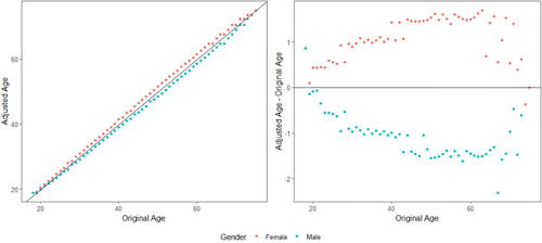
As shown on the left side of Figure 1, before adjusting with the DI remover, the driver population has a higher proportion of young women than young men and, correspondingly, a relatively larger proportion of the older driver population are male drivers. The DI remover aims to remove the effect of gender on age, and, in general, men’s ages are adjusted downward and women’s ages are adjusted upward as displayed in Figure 2. One important property of the DI remover is that it strongly preserves rank among male or female policyholders. However, there is a question of legitimacy here; that is, whether adjusting the age of policyholders is a reasonable action. Alternative methods to remove disparate impact include reweighting and resampling (Kamiran and Calders 2012).

Figure 1. Probability Density Plots of Age by Gender Before and after Adjusting for Age Using the DI Remover.

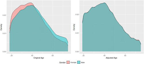
Figure 2. The Effect of DI Remover by Age and Gender.

5.3. Model Comparison

5.3.1. Model Comparison with the Effects of Gender Proxy

Following Frees and Huang (2021), we develop an artificial gender proxy¹¹ for the probability of being female for each driver that takes into account 10 moderately efficient gender proxy variables¹² that are simulated independently using the gender information of each observation. This gender proxy is created based on the idea that the accumulation of some medium proxy variables will form a strong gender proxy. Although it may constitute indirect discrimination in the EU under the Gender Directive or intentional discrimination in the United States, this artificial proxy predictor is added to MU, MDP, and MCDP, leading to MU’, MDP’ and, MCDP’, respectively.

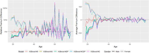
Table 3 displays the means of fitted pure premiums by gender for each pair of model and method, which helps us understand the model performance in terms of group fairness; see Section 3.3. In general, the GLM and XGBoost methods provide similar results in means for each model. M0 as the baseline model displays the biggest discrepancy between male and female distributions. After excluding the use of gender, MU is the only fitting procedure that does not require collecting gender in both training and prediction phases, and, interestingly, women pay higher premiums than men on average as they are on average younger than men in the dataset. MDP achieves the demographic parity criterion and group fairness is ensured, whereas the difference in means almost disappears after removing the influence of gender in all other predictors, as we expected. MCDP is a promising insurance antidiscrimination model as a compromise between MU and MDP, and by introducing legitimate variables, we allow for deviations of group fairness from these predictors. As a better alternative to MU that also focuses on individual fairness, MC performs similar to MU when there is no strong gender proxy in the training data. In general, MU, MU’, and MC meet the EU unisex premium standard; that is, the same auto insurance premium will be charged to male and female drivers given the same driver profile.

TABLE 3 Comparison of Means of Predicted Pure Premiums by Model, Method, and Gender after Portfolio-Level Adjustment

	M0	MU	MU’	MDP	MDP’	MCDP	MCDP’	MC
GLM male	130.47	114.03	118.53	117.38	120.78	115.26	119.40	113.95
GLM female	95.66	124.05	116.25	118.23	112.34	121.90	114.73	124.18
XGBoost male	131.06	114.41	118.45	117.74	120.63	116.59	119.97	114.24
XGB female	94.50	123.39	116.37	117.61	112.60	119.61	113.74	123.68

5.3.2. Scenario Analysis: Group Fairness and Prediction Accuracy

To compare the performance of different methods and models, we use root mean square error (RMSE) and normalized Gini index as our model evaluation metrics. Let ${\widehat{y}}_i$ denote the predicted pure premium for observation i; then the RMSE is defined as $$\text{RMSE}=\sqrt{\frac{1}{n}\sum _{i=1}^n{(y_i-{\widehat{y}}_i)}^2}.$$

For a sequence of numbers $\{s_i,\dots ,s_n\},$ we denote $r(s_i)\in \{1,\dots ,n\}$ as the rank of s_i in the sequence in an increasing order, and the normalized Gini index (Ye et al. 2018) is defined as $$\text{Normalized}\mathrm{ }\text{Gini}\mathrm{ }\text{Index}=\frac{\frac{\sum _{i=1}^n{y}_i r({\widehat{y}}_i)}{\sum _{i=1}^n{y}_i}-\sum _{i=1}^n\frac{n-i+1}{n}}{\frac{\sum _{i=1}^n{y}_i r(y_i)}{\sum _{i=1}^n{y}_i}-\sum _{i=1}^n\frac{n-i+1}{n}}.$$

Therefore, the normalized Gini index utilizes pure premium predictions (${\widehat{y}}_i$) only through their relative orders, and a larger normalized Gini index indicates better model predictions.

In parallel, we also introduce a model fairness measure to indicate how well each model performs on group fairness inspired by RDP, and we call this the disparate impact ratio, which is defined as follows: $$\text{Disparate}\mathrm{ }\text{Impact}\mathrm{ }\text{Ratio}=\frac{\mathbb{E}(\widehat{Y}=\widehat{y}|X_P=b)}{\mathbb{E}(\widehat{Y}=\widehat{y}|X_P=a)}.$$

To approximate the insurance version of the four-fifths rule, we expect this fairness score to be in the range of 0.8 to 1.25. In other words, we hope the difference in premiums on average between groups a and b does not deviate too much.

In total, we consider four different scenarios to show the effects of antidiscrimination pricing models with respect to group fairness (demographic parity) and prediction accuracy. Three scenarios (Scenarios 1–3) are created by choosing different legitimate predictors in MCDP, and an extra scenario (Scenario 4) is created by adding an additional gender proxy to all five models to make MC more differentiable compared to MU.

• Scenario 1: let Insurance Score be the only nonlegitimate predictor in MCDP, and we consider Scenario 1 as our baseline scenario;

• Scenario 2: let both Insurance Score and Density be nonlegitimate in MCDP;

• Scenario 3: let Age be the only non-legitimate variable in MCDP;

• Scenario 4: an artificially created Gender Proxy is added in all models, and let the Gender Proxy be the only nonlegitimate predictor in MCDP.

The fairness–accuracy plots are shown in Figures 3 to 6. In each left-hand side plot, a larger value of RMSE represents a more accurate model, whereas for each right-hand side plot, a smaller value of the normalized Gini index represents a more accurate model. In MDP and MCDP, we preadjust all or some of the nonprotected predictors using the DI remover to make them gender-neutral by removing their dependence on Gender, and we note that adjusting an individual predictor may either improve or reduce the accuracy and fairness of the model. Overall, the effect of adjusting for Age or Insurance Score is positive due to improved fairness and accuracy, whereas the effect is negative for Density due to decreased accuracy¹³.

In Scenarios 1 to 3, MU and MC perform similarly and their model performance is different only when there is at least one moderate gender proxy in the training data, so we add an artificially created gender proxy in all models in Scenario 4. It can be noticed that the effect of this gender proxy is different when using the GLM and XGBoost methods. Our empirical analysis shows that the XGBoost method is generally more sensitive to small gender-related differences, and we suggest that insurance regulators or practitioners need to be aware that different pricing methods may have different degrees of sensitivity to the protected variable. This finding echoes the recommendation given in the EIOPA (2019) report that EU regulators consider the option of introducing specific governance requirements for specific BDA tools and algorithms.

In Scenario 4, MCDP and MC perform similarly in terms of fairness, whereas MCDP outperforms MC (especially for XGBoost) slightly in terms of accuracy when the gender proxy is introduced in the data. We also notice that MCDP and MC perform similarly in terms of both accuracy and fairness when there is a strong gender proxy in the training set.

Overall, M0 has the best prediction accuracy and worst group fairness in all scenarios. XGBoost has better prediction accuracy compared to GLM. Because MU, MDP, MCDP, and MC all satisfy the four-fifths rule according to RDP in all scenarios (within the dotted lines in Figures 3–6), we could select the best model based on their prediction accuracy. In particular, XGBoost MCDP achieves the best trade-off in Scenarios 1 and 3. XGBoost MU and MC (MDP comes the third) achieve the best trade-off in Scenario 2. XGBoost MU (MCDP comes second) achieves the best trade-off in Scenario 4.

Figure 3. Fairness–Accuracy Plot (Scenario 1).

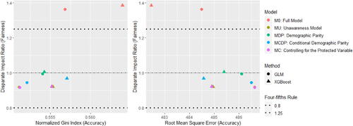
Figure 4. Fairness–Accuracy Plot (Scenario 2).

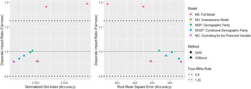
Figure 5. Fairness–Accuracy Plot (Scenario 3).

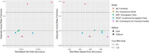
Figure 6. Fairness–Accuracy Plot (Scenario 4).

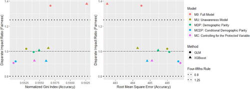
5.3.3. Adverse Selection and Solidarity

Insurance practitioners may be concerned that the use of fair models will harm the principle of actuarial (individual) fairness and lead to adverse selection as a result of implementing antidiscrimination pricing models. Following Goldburd et al. (2016), double lift charts are drawn to compare the relative performance of the two models. Although the implementation of a fair model can be either nonmandatory or mandatory in regulations, the following analysis assumes a nonmandatory implementation of a fair model. We analyze adverse selection and consumer behavior by comparing fair models with the common unawareness practice, and the competitor (benchmark) model is assumed to be GLM MU. We use Scenario 1 as an example for illustration purposes throughout this section. The steps for creating a double lift chart are as follows:

1. We find the pure premium ratio for each individual based on a pair of benchmark and fair models and sort the ratios from lowest to highest. The pure premium ratio is defined as a comparison of predicted pure premiums of one model to another model for the same policyholder. $$\text{Pure}\mathrm{ }\text{Premium}\mathrm{ }\text{Ratio}=\frac{\text{Predicted}\mathrm{ }\text{Premium}\mathrm{ }\text{of}\mathrm{ }\text{Benchmark}\mathrm{ }\text{Model}}{\text{Predicted}\mathrm{ }\text{Premium}\mathrm{ }\text{of}\mathrm{ }\text{Fair}\mathrm{ }\text{Model}}.$$

2. We create bins of equal volume exposure based on the pure premium ratios calculated.

3. For each bin, we calculate the average predicted premium for each model and the average actual experience based on actual claims.

Double lift charts are created separately by gender to compare the rating plans of the benchmark model to a fair model. The first and last bins from each double lift chart represent the two models that disagree with each other the most, and when an insurance company switches from an unawareness model to a fair model, it is most likely to lose customers from the first bin and gain customers from the last bin. In general, the effects of adverse selection using fair models compared to using the benchmark model are limited and the benefit of fairness may occur. For example, comparing GLM MDP with GLM MU in Figure 7, insurers implementing a fair model will lose relatively high-risk male customers and gain low-risk male customers. And this pattern reverses for females. In Figure 8, we see that the overall pattern is closer to the male one; that is, insurers implementing a fair model will lose relatively high-risk customers and gain low-risk customers. The difference between GLM MCDP and GLM MU is relatively small, see Figures c.1. and C.2 in Appendix C.

Figure 7. Double Lift Charts by Gender (GLM MDP versus GLM MU).

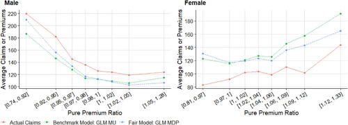
Figure 8. Double Lift Chart (GLM MDP versus GLM MU).

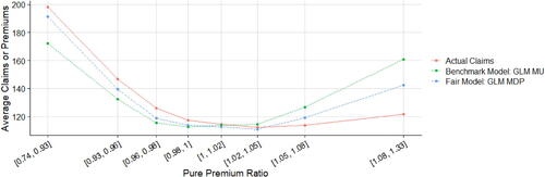
In addition, if the fair model is based on XGBoost (see Figures C.3–C.6 in Appendix C), we notice that insurers implementing XGBoost MDP and XGBoost MCDP will always lose relatively high-risk male customers and gain low-risk customers from both genders. Also, the premium difference from the benchmark GLM MU is larger using XGBoost fair models than using GLM fair models. This is consistent with our findings earlier that XGBoost models have better forecasting performance than GLM models.

Considering adverse selection is from the perspective of the insurance company; in contrast, the concept of solidarity views insurance products from the perspective of the shared responsibility in a community. Insurance products may seek an effective balance between customer segmentation and risk pooling (Henckaerts et al., 2021). Following Henckaerts et al. (2021), we assess the principle of solidarity by comparing the relative and average premium difference of each model by age and gender with respect to the benchmark models, including GLM MU, GLM M0, and actual claims costs; see Figures 9 and10 and Figures C.7 to C.10 in Appendix C. Let ${\overline{Y}}_{\mathit{\text{fair}},i}$ and ${\overline{Y}}_{\mathit{\text{bench}},i}$ denote the average predicted premium of the fair model and benchmark model for age i, respectively. We define relative premium difference and average premium difference for age i below: $$\begin{array}{c}\text{Relative}\mathrm{ }\text{Premium}\mathrm{ }\text{Difference}\mathrm{ }\text{for}\mathrm{ }\text{age\hspace{0.17em}}i=\frac{{\overline{Y}}_{\mathit{\text{fair}},i}-{\overline{Y}}_{\mathit{\text{bench}},i}}{{\overline{Y}}_{\mathit{\text{bench}},i}},\\ \text{Average}\mathrm{ }\text{Premium}\mathrm{ }\text{Difference}\mathrm{ }\text{for}\mathrm{ }\text{age\hspace{0.17em}}i={\overline{Y}}_{\mathit{\text{fair}},i}-{\overline{Y}}_{\mathit{\text{bench}},i}.\end{array}$$

Figure 9. Relative and Average Premium Difference (GLM Models versus GLM MU).

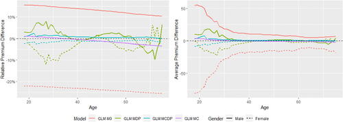
Figure 10. Relative and Average Premium Difference (GLM Models versus GLM M0).

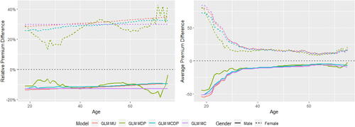
MDP, which focuses on group fairness, is theoretically the best model for the solidarity principle. It is clear from Figure 9 that, compared to GLM MU, the main subsidy of GLM MDP is from males to females (except for older ages) to ensure group fairness among genders and mostly between young people in terms of dollar amount (see the right-hand side of Figure 9). However, compared to GLM M0 (see Figure 10), all other GLM fair models have the subsidy from females to males. Similar patterns can be observed when using XGBoost as fair models; see Figures C.7 and C.8 in Appendix C. When using the actual claims cost as the benchmark, we see that the patterns are more volatile across ages (see Figures C.9 and C.10 in Appendix C) than the other plots using a fitted model as the benchmark. The reason is that age is fitted as a continuous variable, so the effect of age on predicted premiums has been smoothed out using fitted models. We also notice that young females subsidize young males for most models when using actual claims cost as the benchmark. It is also interesting to see that XGBoost M0 has the smallest average premium difference compared to the actual claims cost over all ages, showing that it is the model that provides the most accurate risk estimates.

6. CONCLUSION

Insurers benefit from the collection of more granular data and the use of more advanced analytics techniques in an age of Big Data, but they are also capable of discriminating against protected classes more efficiently in underwriting or pricing decisions. In this article, we have established a connection between various insurance regulations, fairness criteria, and antidiscrimination insurance pricing models; in particular, we have matched the traditional conflict between individual and group fairness with the opposing views on antidiscrimination regulations between high-risk consumers (or regulators) and insurers, which also reflects the different views of insurance in different contexts: economic commodity or social good (Frees and Huang, 2021).

Our empirical analysis using both GLM and XGBoost compares the outcome of different models and analyzes their impact from the perspectives of fairness–accuracy trade-off, adverse selection, and solidarity. Overall, M0 has the best prediction accuracy and worst group fairness in all scenarios and XGBoost has better prediction accuracy compared to GLM. We also find that MU, MDP, MCDP, and MC all satisfy the four-fifths rule in all scenarios considered in this article and different models can achieve the best trade-off under different scenarios. We also find that GLM and XGBoost may have different sensitivity to protected variables. For example, the XGBoost method is generally more sensitive to small gender-related differences, and we suggest that insurance regulators or practitioners need to be aware that different pricing methods may have different degrees of sensitivity to the protected variable. We find that in certain scenarios analyzed in the article, insurers implementing a fair model will lose relatively high-risk customers and gain low-risk customers for both GLM and XGBoost models. Fairness is achieved mostly via the subsidy from young females to young males considering the actual claims cost as the benchmark.

This research contributes to the understanding and mitigation of indirect discrimination in the insurance industry and we propose some research directions for future work. First, antidiscrimination regulations vary across different lines of business and jurisdictions, whereas our research primarily focuses on general insurance. Other lines of business are worthy of further study. Second, one practical difficulty is how to collect protected policyholder information (such as race or ethnicity), and Lindholm et al. (2022a) indicated that indirect insurance discrimination can be caused by incomplete discriminatory information. Recently, several methods in the machine learning field have been proposed to deal with this issue; see Kallus, Mao, and Zhou (2021) and Wang et al. (2020). More research in the insurance domain is needed. Third, future studies may further investigate the impacts of new technologies and innovations on insurance discrimination issues, such as telematics on auto insurance (i.e., more positive impacts) or genetic testing on life and health insurance (i.e., potential negative impacts). Fourth, the existing literature on fair insurance pricing that has emerged in recent years focuses predominantly on cost modeling (or pure premium). However, the final market prices may deviate significantly for policyholders with the same estimated pure premium, especially when non-risk-based price discrimination is allowed (Thomas 2012). Another interesting area is to understand the implications of different fairness criteria and regulations for stakeholders considering the entire pricing process; for example, see Shimao and Huang (2022).

ACKNOWLEDGMENTS

The authors are grateful to the anonymous reviewers and editor for their constructive comments. The authors thank Chris Dolman, Edward (Jed) Frees, and Michael Powers for valuable comments and suggestions and various seminar participants for helpful comments.

Notes

1 Birnbaum (2020b) made a similar point in his presentation to the National Association of Insurance Commissioners Consumer Liaison Committee, and asked, "If discriminating intentionally on the basis of prohibited classes is prohibited—e.g., insurers are prohibited from using race, religion or national origin as underwriting, tier placement or rating factors—why would practices that have the same effect be permitted?”

2 We believe this is a legal term derived from U.S. employment discrimination laws and is synonymous with intentional discrimination.

3 Note that we use a narrow definition of indirect discrimination assuming that the law has prohibited or will prohibit direct discrimination on protected characteristics, and we limit the scope of our research on indirect discrimination to this situation. We recognize that direct discrimination and indirect discrimination on the same protected characteristic may occur simultaneously, but if direct discrimination is allowed, then the provisions on indirect discrimination will be meaningless.

4 Although it may cover intentional indirect discrimination, it is too difficult to prove discriminatory intent under a disparate treatment case.

5 EIOPA (2019) noted that “some insurance firms declared that they ‘smoothed’ the output of such algorithms, for instance by not using machine learning without human intervention or by establishing caps to the outputs of these tools in order to ensure ethical outcomes (e.g. not charging vulnerable customers excessively).⋯ Regarding the potential difficulties to access insurance for high-risk consumers,⋯ motor insurance firms also referred to already existing mechanisms in some jurisdictions such as insurability schemes or the obligation of insurance firms to not reject motor third-party liability insurance (MTPL) consumers (albeit there is no limit in maximum premium).”

6 In December 2021, a new Innovation, Cybersecurity, and Technology (H) Committee was formed to address the insurance implications of emerging technologies and cybersecurity. The Big Data and Artificial Intelligence (H) Working Group is part of the H committee; see NAIC (2021).

7 Previously that, on February 8, 2013, the U.S. Department of Housing and Urban Development (HUD) issued a final rule titled “Implementation of the Fair Housing Act’s Discriminatory Effects Standard” (“the 2013 rule”) that authorizes disparate impact claims under the FHA as a formal interpretation of the Act, consistent with HUD’s long-held view. In particular, HUD restated its position that the FHA applies to homeowners insurance, and hence the disparate impact standard is applicable to prohibit discriminatory insurance practices with regards to homeowners insurance.

8 “Proxy discrimination occurs when insurers discriminate based on facially-neutral traits that (i) are correlated with membership in a protected groups, and (ii) are predictive of losses for precisely that reason”. This definition of “proxy discrimination” was submitted by Professor Daniel Schwarcz to the NAIC during the NAIC’s deliberations regarding its Principles on Artificial Intelligence, based on work in Prince and Schwarcz (2019), available at https://33afce.p3cdn2.secureserver.net/wp-content/uploads/2020/11/Prof.-Dan-Schwarcz-Proxy-Discrimination-Definition.pdf.

9 In pg15training, the first 21 records have been removed because they are duplicate records, which have nonzero claim count (Numtppd) and zero claim amount (Indtppd). After removal, there are exactly 50,000 policies each year in 2009 and 2010.

10 In France, each policyholder is assigned a starting bonus–malus coefficient (a.k.a., coefficient de réduction-majoration in French, abbreviated as CRM) of 1.00 under the French bonus–malus system, and the range of the coefficients extends from 0.50 (i.e., the maximum no-claims bonus will be obtained after at least 13 consecutive claim-free years without a responsible accident) to 3.50. A bonus—malus coefficient is used to adjust the basic premium of the policyholder from the maximum reduction allowed of 50% to the maximum increase allowed of 350%. The French system rewards a claim-free year by a 5% reduction of the coefficient, which is applied to the coefficient for the previous year, and penalizes each fully responsible accident by a 25% increase of the coefficient and each partially responsible accident by half (i.e., 12.5%). More information about bonus-malus in automobile insurance in France can be found on the Directorate of Legal and Administrative Information (2020).

11 Alternatively, gender proxies can be constructed based on variables in the training sample only (Age is highly influential in the gender proxy in this example). However, in this case the developed proxy is ineffective for MU’, as there is no new information added to MU’ compared to MU.

12 We simulate five male binary proxy variables and five female binary proxy variables. For example, in order to simulate the male proxy variable, given the gender of a person, each male has a 60% chance of being in the positive class, while each female only has a 40% chance.

13 Insurance Score: In Scenario 1, we compare MU with MCDP; Density: we compare MCDP’s performance between Scenarios 1 and 2; Age: in Scenario 3, we compare MU with MCDP.

14 Disparate impact discrimination is also applicable under Title VI. According to the U.S. Department of Transportation (n.d.a, n.d.b), “Disparate impact (also called adverse impact) discrimination happens under Title VI when a recipient of federal funds from FHWA adopts a procedure or engages in a practice that has a disproportionate, adverse impact on individuals who are distinguishable based on their race, color, or national origin–even if the recipient did not intend to discriminate” (https://www.fhwa.dot.gov/civilrights/programs/docs/Title/%20VI/%20-/%20Types/%20of/%20Discrimination.pdf). Similarly, for more detail on the three-step approach regarding how to prove a violation of disparate impact standard under the Title VI, see the Title VI Legal Manual published by the U.S. Department of Justice (2021) (https://www.justice.gov/crt/fcs/T6Manual7/#:∼:text=To/%20establish/%20an/%20adverse/%20disparate,and/%20(4)/%20establish/%20causation).

15 Including Wards Cove Packing Co. v. Atonio, 490 U.S. 642 (1989); see also Civil Rights Act of 1991 (1991) §2(2): “The decision of the Supreme Court in Wards Cove Packing Co. v. Atonio, 490 U.S. 642 (1989) has weakened the scope and effectiveness of Federal civil rights protections”; the Wards Cove case’s precedent was nullified by the 1991 Act Because this precedent would make it extremely difficult for the plaintiff to prove disparate impact claims under Title VII.

16 In particular, in Alexander v. Sandoval, (2001), U.S. Supreme Court Held Title VI statute does not allow for private lawsuits based on disparate impact (https://www.fhwa.dot.gov/civilrights/programs/docs/Title%20VI%20-%20Intentional%20Discrimination%20and%20Disparate%20Impact.pdf).

17 See the 2013 rule, HUD responded to the concerns from the insurance industry that “HUD has long interpreted the Fair Housing Act to prohibit discriminatory practices in connection with homeowner’s insurance, and courts have agreed with HUD, including in Ojo v. Farmers Group (2011). Moreover, as discussed above, HUD has consistently interpreted the Act to permit violations to be established by proof of discriminatory effect. By formalizing the discriminatory effects standard, the rule will not, as one commenter suggested, ‘undermine the states’ regulation of insurance.’⋯ McCarran-Ferguson does not preclude HUD from issuing regulations that may apply to insurance policies.”

18 Civil Case No. 13–00966 (RJL), United States District Court, District of Columbia, signed November 7, 2014 (see https://ecf.dcd.uscourts.gov/cgi-bin/show_public_doc?2013cv0966-47; see also The Lawyers' Committee for Civil Rights Under Law (2015) https://www.lawyerscommittee.org/project/aianamic/). “Judge Leon, accepting plaintiffs’ argument that the FHA only prohibits intentional discrimination and that the McCarran-Ferguson Act forecloses the application of disparate impact theory to the provision of homeowners’ insurance, held the FHA unambiguously forecloses the possibility of disparate impact claims.”

19 See a comprehensive summary for the differences in the HUD’s 2020 Rule and how the Inclusive Communities decision in 2015 is different from the HUD’s 2013 Rule (Friedman 2020) (https://www.jdsupra.com/legalnews/hud-issues-final-rule-on-the-fair-63161/).

20 See the Federal Reserve (2017) (https://www.federalreserve.gov/boarddocs/supmanual/cch/fair_lend_over.pdf): “Redlining is a form of illegal disparate treatment whereby a lender provides unequal access to credit, or unequal terms of credit, because of the race, color, national origin, or other prohibited characteristic(s) of the residents of the area in which the credit seeker resides or will reside or in which the residential property to be mortgaged is located. Redlining may violate both the FHAct and the ECOA [Equal Credit Opportunity Act].”

APPENDIX A.

THE EVOLVEMENT OF U.S. INSURANCE DISCRIMINATION REGULATIONS

On July 6, 2021, Colorado Senate Bill (SB) 21-169 (Colorado Division of Insurance, 2021) was signed into law, and this legislative reform is considered a breakthrough attempt on the issue of indirect insurance discrimination in insurance regulations. In this appendix, we summarize the evolvement of U.S. insurance discrimination regulations, including existing insurance discrimination definitions that have been widely used and some newly proposed definitions being considered by insurance regulators from various stakeholders.

A.1. Part 1. State-Based Insurance Regulation and Unfair Discrimination Statutes

The McCarran-Ferguson Act of 1945 formally delegated regulatory authority from Congress to the states (NAIC 2022) regarding regulation of the business of insurance, and therefore general insurers are regulated predominantly at the state level, including our focus: antidiscrimination laws and regulations in the insurance industry.

Wortham (1986b) reviewed the history of the development of state unfair discrimination statutes in relation to insurance discrimination, which often requires that insurance classification be supported by statistical evidence showing a correlation with loss (in all states in at least some personal lines of insurance). In particular, state insurance laws often require that insurance premiums be fair and not unfairly discriminatory—a general standard that is commonly contained in insurance regulations is that insurance rates shall not be excessive, inadequate, or unfairly discriminatory, usually defined as follows, derived from Section 5A (3) Unfairly Discriminatory Rates of the NAIC Property and Casualty Model Rating Law (GDL-1775; NAIC 2010):

Unfair discrimination exists if, after allowing for practical limitations, price differentials fail to reflect equitably the differences in expected losses and expenses. A rate is not unfairly discriminatory if it is averaged broadly among persons insured under a group, franchise or blanket policy or a mass marketed plan.

As another example, in 1988, p. 2, the CAS published the Statement of Principles Regarding Property and Casualty Insurance Ratemaking, which describes in Principle 4 that “a rate is reasonable and not excessive, inadequate, or unfairly discriminatory if it is an actuarially sound estimate of the expected value of all future costs associated with an individual risk transfer.”

The above principle also corresponds to the actuarial fairness principle, a guiding principle in the insurance industry; see Landes (2015) for more discussion.

A.2. Part 2. Disparate Impact Standard and Its Applicability in the Insurance Industry

Disparate impact, also known as adverse impact, refers to discrimination that is unintentional, and it is a legal term as a means of proving that indirect discrimination has occurred without the need to prove discriminatory intent or motive in a discrimination lawsuit.

In the landmark ruling of Griggs v. Duke Power Co. (1971), the first legal precedent was established for disparate impact claims under Title VII of the Civil Rights Act of 1964 in the employment context. In a disparate impact case for employment discrimination, a three-step burden-shifting approach is adopted¹⁴. First, the plaintiff must establish a prima facie case of adverse disparate impact. It is important to note that even where a disparate impact is shown by a plaintiff at step 1, the practice would not constitute discrimination (or impose liability) if the defendant (i.e., the employer) can demonstrate the practice causing a disparate impact is consistent with business necessity at step 2 (i.e., a business necessity test constitutes a defense to disparate impact claims). Finally, if the employer has successfully passed the business necessity test for their discriminatory practice, the employee then has the opportunity and may still succeed at step 3 if they can show that an alternative practice exists that is comparable and less discriminatory, which the employer refuses to adopt. On November 21, 1991, the disparate impact framework was codified into the Civil Rights Act of 1991 in response to several controversial and adverse U.S. Supreme Court decisions¹⁵ prior to the introduction of the Act. In Smith v. City of Jackson (2005), the U.S. Supreme Court confirmed that the Age Discrimination in Employment Act of 1967 (ADEA) also authorizes disparate impact claims, but “the scope of disparate-impact liability under ADEA is narrower than under Title VII.”

Since the disparate impact theory was proposed, it has generally been believed that the disparate impact standard is only applicable to the field of employment discrimination¹⁶. On February 8, 2013, HUD issued a final rule titled “Implementation of the Fair Housing Act’s Discriminatory Effects Standard” (“the 2013 rule”) that authorizes disparate impact claims under the FHA as a formal interpretation of the Act, consistent with HUD’s long-held view. In particular, HUD restated its position that the Fair Housing Act applies to homeowners insurance¹⁷, and hence the disparate impact standard is applicable to prohibit discriminatory insurance practices with regards to homeowners insurance.

However, the application of the disparate impact standard in the context of the insurance industry is strongly opposed by insurance companies. NAMIC (2017) claimed that the 2013 rule meant to insurers that “any factor used by insurers to assess risk could be challenged if it produced statistically disproportionate outcomes among demographic groups” and argued that “insurers do not even know the race, religion, or national origin of their insureds” (NAMIC 2020). Therefore, NAMIC and the American Insurance Association—two insurance industry trade associations—jointly challenged the validity of HUD’s disparate impact rule under the FHA in the U.S. District Court for the District of Columbia; see American Insurance Association, et al. v. United States Department of Housing and Urban Development, et al. (2014)¹⁸, and scored an initial victory on November 3, 2014.

On June 25, 2015, the U.S. Supreme Court held that disparate impact claims are cognizable under the FHA in the landmark decision of Texas Department of Housing and Community Affairs v. Inclusive Communities Project, Inc. (2015), and NAMIC’s victory at the district court level was overruled by the Supreme Court decision in Inclusive Communities. In April 2016, the plaintiffs filed an amended complaint to challenge the HUD’s disparate impact rule and a summary judgment motion was filed in June 2016 that seeks to “invalidate the 2013 Rule to the extent it applies to insurers’ ratemaking and underwriting decisions” (Willis, Andreano, and Sommerfield 2021) and the lawsuit has been pending in the D.C. federal district court since June 2018 for HUD’s revisions to the 2013 rule.

On September 24, 2020, HUD (2020) issued a final rule titled “HUD’s Implementation of the Fair Housing Act’s Disparate Impact Standard” (“the 2020 rule”) that amended the 2013 rule, including the “clarification regarding the application of the standard to state laws governing the business of insurance.” Since being proposed, the 2020 rule has been widely criticized by consumer advocates and Democratic lawmakers because it requires a heavy burden of proof on the plaintiff for a disparate impact claim under the Fair Housing Act¹⁹ and appears to favor the defendant, and therefore there are at least three lawsuits challenging the 2020 rule in federal district courts. On January 26, 2021, President Biden issued an executive order (White House 2021) to direct HUD to review the effects of the 2020 rule, including the effect of revising the 2013 rule. On June 25, 2021, HUD formally proposed to rescind the 2020 rule and restore the 2013 rule (HUD 2021).

In terms of the definition, the United States does not clearly define disparate impact (even indirect discrimination) in statute law. In short, disparate impact describes “when a facially neutral practice that has an unjustified adverse impact on members of a protected class” (Fick 1997, p. 21) In other fields—for example, with regard to fair lending—the Federal Reserve (2017) interprets disparate treatment and disparate impact with respect to lending discrimination under the Equal Credit Opportunity Act and the FHA as follows:

Disparate Treatment: The existence of illegal disparate treatment may be established either by statements revealing that a lender explicitly considered prohibited factors (overt evidence) or by differences in treatment that are not fully explained by legitimate nondiscriminatory factors (comparative evidence).

Disparate Impact: A disparate impact occurs when a lender applies a racially (or otherwise) neutral policy or practice equally to all credit applicants but the policy or practice disproportionately excludes or burdens certain persons on a prohibited basis.⋯ Although the law on disparate impact as it applies to lending discrimination continues to develop, it has been clearly established that a policy or practice that creates a disparity on a prohibited basis is not, by itself, proof of a violation.

To sum up, we believe the definition of disparate treatment includes direct discrimination and some intentional indirect discrimination. Disparate impact is a subset of indirect discrimination because it is a legal definition and only intends to cover unintentional discrimination (although it may cover intentional indirect discrimination, it is too difficult to prove discriminatory intent under a disparate treatment case). For example, redlining as a classic example of indirect discrimination (or proxy discrimination) is a form of (illegal) disparate treatment,²⁰ rather than disparate impact.

A.3. Part 3. Colorado Bill and Recent Regulatory Reform Discussion

On August 14, 2020, the NAIC (2020b) published guiding principles on AI, including a key principle “encouraging industry participants to take proactive steps to avoid proxy discrimination against protected classes when using AI platforms” (NAIC, 2020a) developed by the NAIC’s Big Data and Artificial Intelligence Working Group. Specifically, as part of the “fair and ethical” tenet, one key NAIC’s AI principle is outlined below:

Consistent with the risk-based foundation of insurance, AI actors should proactively engage in responsible stewardship of trustworthy AI in pursuit of beneficial outcomes for consumers and to avoid proxy discrimination against protected classes. AI systems should not be designed to harm or deceive people and should be implemented in a manner that avoids harmful or unintended consequences and corrects and remediates for such consequences when they occur.

However, the term “proxy discrimination” has not yet been defined by the NAIC, and it is unclear to insurers how to comply with the guiding principles to avoid proxy discrimination in practice. In addition, the guiding principle covers “unintended consequences,” which could upend the industry’s understanding of indirect discrimination, whereas insurance antidiscrimination laws were previously thought to have generally focused on direct discrimination and intentional indirect discrimination.

A recent example is the Colorado Senate Bill 21-169 (Colorado Division of Insurance 2021) in the United States, which was passed and signed into law in July 2021, and its definition of unfair discrimination, which has a “disparate impact” component, outlined as follows:

“Unfairly discriminate” and “unfair discrimination” include the use of one or more external consumer data and information sources, as well as algorithms or predictive models using external consumer data and information sources, that have a correlation to race, color, national or ethnic origin, religion, sex, sexual orientation, disability, gender identity, or gender expression, and that use results in a disproportionately negative outcome for such classification or classifications, which negative outcome exceeds the reasonable correlation to the underlying insurance practice, including losses and costs for underwriting.

The above definition could be the first insurance regulation to focus on the effects of discrimination at the group level, which is common in other areas such as lending, housing, and college admissions.

A.4. Part 4. Other Restrictions or Regulatory Requirements

Some other more specific or broad regulations or regulatory requirements that cannot be classified into the regulations discussed in Section 2.5 are listed below:

1. Regulatory Prior Approval. Compared with no regulation, a more realistic minimum standard for insurance companies is that the variables they use need to be approved in advance by regulators. In the United States, a general standard is that insurance rates shall not be excessive, inadequate, or unfairly discriminatory (NAIC, 2010), and state regulators usually require insurance companies to prove that all rating factors are actuarially sound by their predicted value of future losses; exceptions are made for certain protected variables that require (special) social protection, even if these variables are actuarially justified.

2. Regulatory Prior Approval Factors. A more comprehensive approach to prohibiting the use of protected or proxy variables is to provide insurance companies with a list of acceptable factors to choose from. In California, according to Proposition 103, automobile insurers should consider three mandatory rating factors more heavily than other factors in decreasing order of importance: (1) the insured’s driving safety record, (2) the number of miles he or she drives annually, and (3) the number of years of driving experience the insured has; in addition, insurers are allowed to use 15 optional rating factors including the type of vehicle, type of use of vehicle, vehicle characteristics, academic standing, and marital status of the rated driver; see California Code of Regulations (2023) (Title 10, Section 2632.5). As for another more restrictive example, under the ACA, insurers are only allowed to consider the insureds’ family size, rating area, age, and smoking status, and this practice in the health care system is also known as adjusted community rating because the use of health status, claims experience, or gender is not allowed.

3. Prohibition as a Sole Factor. Insurers can be prohibited from using a certain factor as the sole basis in underwriting or rating decisions, such as ZIP code or credit score, and this regulation can be regarded as a special way of restricting protected or proxy variables.

4. Disparate Impact Standard with Flexibility (e.g., the Four-Fifths Rule). Corresponding to CDP in Section 3 and MCDP in Sections 4 and 5, this regulation is a relaxation of the disparate impact standard because it is less rigorous, and if applied to the insurance field, insurance companies will be allowed to legally deviate from group fairness criterion to a certain extent. As a classic example in the employment context, the Four-Fifths Rule is codified in the 1978 Uniform Guidelines for Employee Selection Procedures (U.S. Government Publishing Office 2017) as follows:

   a selection rate for any race, sex, or ethnic group which is less than four-fifths (4/5) (or eighty percent) of the rate for the group with the highest rate will generally be regarded by the Federal enforcement agencies as evidence of adverse impact, while a greater than four-fifths rate will generally not be regarded by Federal enforcement agencies as evidence of adverse impact.

   Currently, this method is often used along with more rigorous statistical tests and has been applied in many other fields as a reference dividing line of disparate impact.

5. Restriction on the Influence of Protected (or Proxy) Variables. For example, as discussed above, California’s Proposition 103 requires insurance companies to base automobile insurance premiums primarily upon three mandatory rating factors within the driver’s control (specifically, insurers should perform a sequential analysis; see Hunstad [1996] and California Department of Insurance [2020]).

6. Effective Prohibition through Insurance Companies. For various reasons, some insurance companies may voluntarily not use certain protected variables (e.g., occupation and educational level), and if major insurers do not use or collect a specific protected (or proxy) variable, this variable is effectively prohibited, although it is not regulated by laws or regulations.

APPENDIX B.

IMPLEMENTATION DETAILS OF GENERALIZED LINEAR MODELS AND EXTREME GRADIENT BOOSTING

B.1. Generalized Linear Models

Generalized linear models have been widely used by actuaries in general insurance pricing. In this article, we adopt the classical frequency–severity approach by building two separate frequency and severity models. Following De Jong and Heller (2008) and Frees, Derrig, and Meyers (2014), the structure of GLMs is as follows: $$\hspace{1em}g(\mu )=x\prime \beta .$$

Let Y denote the response variable, x the explanatory variables, and μ the expectation of Y, where its distribution is a member of the exponential family of distributions, and let $g(·)$ denote the monotonic link function. To illustrate frequency and severity models, let N denote the number of claims, E the exposures, and S the (aggregate) claim amount. For a claim frequency model, we adopt the Poisson regression model, which is typically applied for count data, with an offset term for exposures: $$N\sim \text{Poisson}(\lambda ),\hspace{1em}\mathit{\text{ln}}(\lambda )=\mathit{\text{ln}}(E)+x{\prime }_F{\beta }_F,$$ where x_F is the set of covariates used in modeling frequency and β_F is the corresponding set of regression coefficients. The claim count N follows a Poisson distribution, and the log link is chosen as $g(·)=\mathit{\text{ln}}(·),$ and logarithmic exposure is added as an offset variable accounting for the premium is proportional to the exposures. For a claim severity model, we apply the gamma regression model for claim size conditional on the event that there is at least one claim filed by policyholders (i.e., N > 0): $$S/N\sim \text{Gamma}(\alpha ,\gamma ),\hspace{1em}\mathit{\text{ln}}(\alpha )=x{\prime }_S{\beta }_S,$$ where x_S is the set of covariates used in modeling severity and β_S is the corresponding set of regression coefficients, and the sets of covariates are not necessarily the same for the frequency and severity models. The claim size S/N follows a gamma distribution, also with a logarithmic link function $g(·)=\mathit{\text{ln}}(·).$

B.2. Extreme Gradient Boosting

XGBoost was proposed by Chen and Guestrin (2016) as a novel gradient tree boosting method and has rapidly gained popularity due to its high efficiency in computational speed and predictive performance in applications in many fields, including its superior performance in machine learning competitions on Kaggle.

XGBoost requires building classification and regression trees iteratively, where each subsequent tree (also known as a weaker learner) is trained to predict the residuals of the previous tree so that by building more weak learners sequentially, the training continues and each new tree corrects errors in the previous tree until a stopping criterion is reached. In XGBoost, assuming we have K additive functions (or trees), a tree ensemble model using K trees is expressed as $$\widehat{Y_i}=\sum _{k=1}^K{f}_k(x_i),\hspace{1em}{f}_k\in \mathcal{F},$$ where $\mathcal{F}$ is the space of functions containing all regression trees and each f_k represents an independent tree structure. The XGBoost method minimizes a regularized objective function as follows (Chen and Guestrin 2016): $$\begin{array}{c}\mathcal{L}=\sum _{i=1}^{n}l(Y_i,\widehat{Y_i})+\sum _{k=1}^K\Omega (f_k)\\ \text{where\hspace{0.17em}}\Omega (f)=\gamma T+\frac{1}{2}\lambda \left|\right|w|{|}^2\end{array}$$ where l is a differentiable convex loss function that measures the difference between the observed outcome Y_i and predicted outcome $\widehat{Y_i},$ and $\Omega (f)$ is the regularization term that penalizes the complexity of the model, where T is the number of leaves in the tree and w is the sum of leaf weights, and γ and λ are the regularization hyperparameters. In addition, the training of the XGBoost model is additive (Chen and Guestrin 2016) and at the $t-\text{th}$ iteration, the objective we aim to minimize is expressed as follows: $${\mathcal{L}}^{(t)}=\sum _{i=1}^{n}l(Y_i,{\widehat{Y_i}}^{(t-1)}+f_t(x_i))+\Omega (f_t),$$ where ${\widehat{Y_i}}^{(t-1)}$ is the prediction at the $(t-1)\text{th}$ iteration. For more mathematical details on implementing the XGBoost method, we refer interested readers to Chen and Guestrin (2016). We fit XGBoost models using the Xgboost package (Chen et al. 2015) in R. To apply XGBoost to insurance pricing, the loss functions for claim frequency and severity models need to be appropriately specified. In fact, the choice of learning objective function in XGBoost is similar to the choice of the distributions of Y in GLMs, and we set the learning objective to count:poisson (Poisson regression) for claim count and reg:gamma (gamma regression with log-link) for claim size. For all XGBoost models, we perform a grid search for tuning hyperparameters by steps using fivefold cross-validation; we refer interested readers to Fauzan and Murfi (2018) for detailed grid search scheme.

APPENDIX C.

SUPPLEMENTARY FIGURES TO SECTION 5

Figure C.1. Double Lift Charts by Gender (GLM MCDP versus GLM MU).

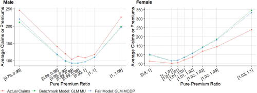
Figure C.2. Double Lift Chart (GLM MCDP versus GLM MU).

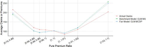
Figure C.3. Double Lift Charts by Gender (XGBoost MDP versus GLM MU).

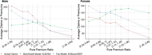
Figure C.4. Double Lift Chart (XGBoost MDP versus GLM MU).

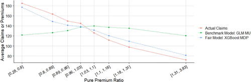
Figure C.5. Double Lift Charts by Gender (XGBoost MCDP versus GLM MU).

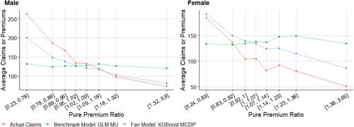
Figure C.6. Double Lift Chart (XGBoost MCDP versus GLM MU).

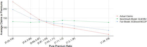
Figure C.7. Relative and Average Premium Difference (XGBoost Models versus GLM MU).

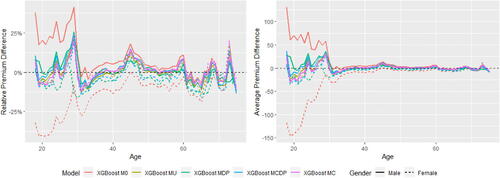
Figure C.8. Relative and Average Premium Difference (XGBoost Models versus GLM M0).

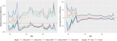
Figure C.9. Relative and Average Premium Difference (GLM Models vs. Actual Claim Costs).

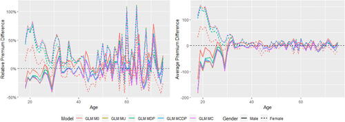
Figure C.10. Relative and Average Premium Difference (XGBoost Models versus Actual Claim Costs).

REFERENCES

- Agarwal, A., M. Dudik, and Z. S. Wu. 2019. Fair regression: Quantitative definitions and reduction-based algorithms. Proceedings of the International Conference on Machine Learning 97:120–29.
- Alexander v. sandoval (No. 99-1908; Vol. 532, p. 275). (2001). (Vol. 532). Supreme Court. https://www.supremecourt.gov/opinions/boundvolumes/532bv.pdf
- AMERICAN INS. V. US DEPT. OF HOUSING AND URBAN (Civil Case No. 13-00966 (RJL); Vol. 74, p. 30). (2014). (Vol. 74). Dist. Court, Dist. of Columbia. https://ecf.dcd.uscourts.gov/cgi-bin/show_public_doc?2013cv0966-47
- Araiza Iturria, C. A., M. Hardy, and P. Marriott. 2022. A discrimination-free premium under a causal framework. 10.2139/ssrn.4079068
- Australian Human Rights Commission. 2020. Using artificial intelligence to make decisions: Addressing the problem of algorithmic bias. https://humanrights.gov.au/sites/default/files/document/publication/ahrc_technical_paper_algorithmic_bias_2020.pdf.
- Australian Human Rights Commission. n.d.a. Direct discrimination. https://humanrights.gov.au/quick-guide/12026.
- Australian Human Rights Commission. n.d.b. Indirect discrimination. https://humanrights.gov.au/quick-guide/12049.
- Australian Law Reform Commission. 2003. Essentially yours—The protection of human genetic information in Australia. Vols. 1 and 2. Report 96. https://www.alrc.gov.au/publication/essentially-yours-the-protectionof-human-genetic-information-in-australia-alrc-report-96/%7D.
- Avraham, R., K. D. Logue, and D. Schwarcz. 2014a. Towards a universal framework for insurance anti-discrimination laws. Connecticut Insurance Law Journal 21:1.
- Avraham, R., K. D. Logue, and D. Schwarcz. 2014b. Understanding insurance antidiscrimination laws. Southern California Law Review 87 (2):195–274.
- Barocas, S., M. Hardt, and A. Narayanan. 2019. Fairness and machine learning. fairmlbook.org.
- Barocas, S., and A. D. Selbst. 2016. Big data’s disparate impact. California Law Review 104:671.
- Berk, R. 2009. The role of race in forecasts of violent crime. Race and Social Problems 1 (4):231–42. 10.1007/s12552-009-9017-z
- Berk, R., H. Heidari, S. Jabbari, M. Joseph, M. Kearns, J. Morgenstern, S. Neel, and A. Roth. 2017. A convex framework for fair regression. arXiv Preprint arXiv:1706.02409.
- Berk, R., H. Heidari, S. Jabbari, M. Kearns, and A. Roth. 2018. Fairness in criminal justice risk assessments: The state of the art. Sociological Methods & Research 50 (1):3–44.
- Binns, R. 2018. Fairness in machine learning: Lessons from political philosophy. Proceedings of Machine Learning Research 81:149–59.
- Binns, R. 2020. On the apparent conflict between individual and group fairness. In Proceedings of the 2020 Conference on Fairness, Accountability, and Transparency, 514–24. New York, NY: Association for Computing Machinery.
- Birnbaum, B. 2020a. Addressing systemic racism in insurance: Presentation to the NAIC committee on race and insurance workstream 4: Life insurance and annuities. https://content.naic.org/sites/default/files/call_materials/cej_presentation_naic_race_life_201210.pdf.
- Birnbaum, B. 2020b. Insurance consumer protection issues resulting from, or heightened by COVID-19: Presentation to NAIC Consumer Liaison Committee. https://content.naic.org/sites/default/files/call_materials/Slideshow_Consumer%5B1%5D.pdf.
- California Department of Insurance. 2020. Private passenger auto class plan filing instructions. http://www.insurance.ca.gov/0250-insurers/0800-rate-filings/upload/Class-Plan-Instructions-02_10_2020.pdf.
- California Office of Administrative Law. (2023). California code of regulations. https://govt.westlaw.com/calregs/Document/IDE21D4235C2F11EC9C68000D3A7C4BC3?viewType=FullText&originationContext=documenttoc&transitionType=CategoryPageItem&contextData=(sc.Default)
- Casualty Actuarial Society. (1988). Statement of principles regarding property and casualty insurance ratemaking. https://www.casact.org/sites/default/files/2021-05/Statement-Of-Principles-Ratemaking.pdf
- Casualty Actuarial and Statistical (C) Task Force. 2015. Casualty Actuarial and Statistical (C) Task Force price optimization white paper. https://content.naic.org/sites/default/files/inline-files/committees_c_catf_related_price_optimization_white_paper.pdf.
- Caton, S., and C. Haas. 2020. Fairness in machine learning: A survey. arXiv Preprint arXiv:2010.04053.
- Centers for Medicare & Medicaid Services. 2022. Market rating reforms—State specific geographic rating areas. https://www.cms.gov/CCIIO/Programs-and-Initiatives/Health-Insurance-Market-Reforms/state-gra.
- Chen, T., and C. Guestrin. 2016. XGBoost: A scalable tree boosting system. In Proceedings of the 22nd ACM SIGKDD International Conference on Knowledge Discovery and Data Mining, 785–94. New York, NY: Association for Computing Machinery.
- Chen, T., T. He, M. Benesty, V. Khotilovich, Y. Tang, H. Cho, K. Chen, R. Mitchell, I. Cano, T. Zhou, et al. 2015. XGBoost: Extreme gradient boosting. R Package v0.4-2. https://cran.microsoft.com/snapshot/2022-01-01/web/packages/xgboost/xgboost.pdf.
- Chiappa, S. 2019. Path-specific counterfactual fairness. Proceedings of the AAAI Conference on Artificial Intelligence 33:7801–8. 10.1609/aaai.v33i01.33017801
- Chibanda, K. F. 2022. SB21-169—Protecting consumers from unfair discrimination in insurance practices. https://doi.colorado.gov/for-consumers/sb21-169-protecting-consumers-from-unfair-discrimination-in-insurance-practices.
- Civil rights act of 1991. (1991). Public Law 102-166. https://www.eeoc.gov/civil-rightsact-1991-original-text#:∼:text=To%20amend%20the%20Civil%20Rights,actions%2C%20and%20for%20other%20purposes.
- Consumer Reports. 2021. Effects of varying education level and job status on online auto insurance price quotes. https://advocacy.consumerreports.org/wp-content/uploads/2021/01/Auto-Insurance-White-Paper-Report-FINAL1.26C.pdf.
- Corbett-Davies, S., E. Pierson, A. Feller, S. Goel, and A. Huq. 2017. Algorithmic decision making and the cost of fairness. In Proceedings of the 23rd ACM SIGKDD International Conference on Knowledge Discovery and Data Mining, 797–806. New York, NY: Association for Computing Machinery.
- Council of the European Union. (2000). Council directive 2000/43/EC of 29 june 2000 implementing the principle of equal treatment between persons irrespective of racial or ethnic origin. https://eur-lex.europa.eu/legal-content/EN/TXT/?uri=celex%3A32000L0043
- Council of the European Union. 2004. Council Directive 2004/113/EC of 13 December 2004 implementing the principle of equal treatment between men and women in the access to and supply of goods and services. https://eur-lex.europa.eu/legal-content/EN/TXT/?uri=celex%3A32004L0113.
- Court of Justice. 2011. Judgment of the Court (Grand Chamber) of 1 March 2011. https://eurlex.europa.eu/legal-content/EN/ALL/?uri=CELEX%3A62009CJ0236, Judgement of the Court, Case C-236/09.
- De Jong, P., and G. Z. Heller. 2008. Generalized linear models for insurance data. New York, NY: Association for Computing Machinery. Cambridge Books.
- Department of Housing and Urban Development. 2013. Implementation of the Fair Housing Act’s discriminatory effects standard. https://www.hud.gov/sites/documents/DISCRIMINATORYEFFECTRULE.PDF.
- Department of Housing and Urban Development. 2020. HUD’s implementation of the Fair Housing Act’s disparate impact standard. https://www.govinfo.gov/content/pkg/FR-2020-09-24/pdf/2020-19887.pdf.
- Department of Housing and Urban Development. 2021. Reinstatement of HUD’s discriminatory effects standard. https://www.federalregister.gov/documents/2021/06/25/2021-13240/reinstatement-of-huds-discriminatory-effects-standard.
- Department of Justice. (2021). Title VI legal manual. https://www.justice.gov/crt/fcs/T6Manual7#:%20:text=To/%20establish/%20an/%20adverse/%20disparate,and/%%20Q201%2020(4)/%20establish/%20causation
- Department of Transportation. (n.d.a). Title VI - intentional discrimination and disparate impact. https://www.fhwa.dot.gov/civilrights/programs/docs/Title%20VI%20-%20Intentional%20Discrimination%20and%20Disparate%20Impact.pdf
- Department of Transportation. (n.d.b). What types of discrimination are prohibited by title VI? https://www.fhwa.dot.gov/civilrights/programs/docs/Title%20VI%20-%20Types%20of%20Discrimination.pdf
- Directorate of Legal and Administrative Information. (2020). Bonus-malus in car insurance. https://www.service-public.fr/particuliers/vosdroits/F2655.
- Di Stefano, P. G., J. M. Hickey, and V. Vasileiou. 2020. Counterfactual fairness: Removing direct effects through regularization. arXiv Preprint arXiv:2002.10774.
- Directorate of Legal and Administrative Information. 2022. Assurance auto obligatoire ou “au tiers” [Compulsory or "third party" car insurance]. https://www.service-public.fr/particuliers/vosdroits/F2628.
- Dolman, C., and D. Semenovich. 2019. Algorithmic fairness: Some practical considerations for actuaries. Paper presented at Actuaries Summit 2019, Sydney, New South Wales, Australia, June 3–4.
- Dunn, R. A. 2009. Measuring racial disparities in traffic ticketing within large urban jurisdictions. Public Performance & Management Review 32 (4):537–61. 10.2753/PMR1530-9576320403
- Dutang, C., A. Charpentier, and M. C. Dutang. 2015. Package “CASdatasets.” http://dutangc.perso.math.cnrs.fr/RRepository/pub/web/CASdatasets-manual.pdf.
- Dwork, C., M. Hardt, T. Pitassi, O. Reingold, and R. Zemel. 2012. Fairness through awareness. In Proceedings of the 3rd Innovations in Theoretical Computer Science Conference, 214–26. New York, NY: Association for Computing Machinery.
- Elliott, M. N., P. A. Morrison, A. Fremont, D. F. McCaffrey, P. Pantoja, and N. Lurie. 2009. Using the Census Bureau’s surname list to improve estimates of race/ethnicity and associated disparities. Health Services and Outcomes Research Methodology 9 (2):69–83. 10.1007/s10742-009-0047-1
- European Commission. 2014. Commission Staff working document Annexes to the joint report on the application of the racial equality directive (2000/43/EC) and the employment equality directive (2000/78/EC). https://eur-lex.europa.eu/legal-content/EN/TXT/?uri=celex:52014SC0005.
- European Insurance and Occupational Pensions Authority. 2019. Big data analytics in motor and health insurance: A thematic review. https://register.eiopa.europa.eu/Publications/EIOPA_BigDataAnalytics_ThematicReview_April2019.pdf.
- Fang, H., and A. Ko. 2018. Partial rating area offering in the ACA marketplaces: Facts, theory and evidence. Cambridge, MA: National Bureau of Economic Research.
- Fauzan, M. A., and H. Murfi. 2018. The accuracy of XGBoost for insurance claim prediction. International Journal of Advances in Soft Computing and Its Applications 10 (2):159–171.
- Federal Reserve. 2017. Fair lending regulations and statutes: Overview. https://www.federalreserve.gov/boarddocs/supmanual/cch/fair_lend_over.pdf.
- Feldman, M., S. A. Friedler, J. Moeller, C. Scheidegger, and S. Venkatasubramanian. 2015. Certifying and removing disparate impact. In Proceedings of the 21th ACM SIGKDD International Conference on Knowledge Discovery and Data Mining, 259–68. New York, NY: Association for Computing Machinery.
- Fick, B. (1997). American bar association guide to workplace law. Times Books, New York, United States.
- Frees, E. W., R. A. Derrig, and G. Meyers. 2014. Predictive modeling applications in actuarial science. Vol. 1. New York, NY: Cambridge University Press.
- Frees, E. W., and F. Huang. 2021. The discriminating (pricing) actuary. North American Actuarial Journal. 27 (1):2–24
- Friedman, C. (2020). HUD issues final rule on the fair housing act’s disparate impact standard. https://www.jdsupra.com/legalnews/hud-issues-final-rule-on-the-fair-63161/.
- Gaulding, J. 1994. Race sex and genetic discrimination in insurance: What’s fair. Cornell Law Review 80:1646.
- Goldburd, M., A. Khare, D. Tevet, and D. Guller. 2016. Generalized linear models for insurance rating. Arlington, VA: Casualty Actuarial Society, CAS Monographs Series, 5.
- Grari, V., C. Arthur, L. Sylvain, and D. Marcin. 2022. A fair pricing model via adversarial learning. arXiv Preprint arXiv:2202.12008.
- Griggs v. Duke Power Co. No. 124; Vol. 401, p. 424 (1971). Supreme Court. https://tile.loc.gov/storage-services/service/ll/usrep/usrep401/usrep401424/usrep401424.pdf.
- Hardt, M. 2013. Fairness through awareness. https://course.ece.cmu.edu/∼ece734/fall2013/lectures/cmu13-fairness.pdf.
- Hardt, M., E. Price, and N. Srebro. 2016. Equality of opportunity in supervised learning. arXiv Preprint arXiv:1610.02413.
- Hedden, B. 2021. On statistical criteria of algorithmic fairness. Philosophy and Public Affairs 49 (2):209–231. doi:10.1111/papa.12189.
- Henckaerts, R., M.-P. Côté, K. Antonio, and R. Verbelen. 2021. Boosting insights in insurance tariff plans with tree-based machine learning methods. North American Actuarial Journal 25 (2):255–85. 10.1080/10920277.2020.1745656
- Hunstad, L. 1996. Sequential analysis guidelines. https://www.insurance.ca.gov/0250-insurers/0800-rate-filings/upload/Sequential-Analysis.pdf.
- Hutchinson, B., and M. Mitchell. 2019. 50 Years of test (un) fairness: Lessons for machine learning. In Proceedings of the Conference on Fairness, Accountability, and Transparency, 49–58. New York, NY: Association for Computing Machinery.
- Insurance Information Institute. 2019. Background on: Credit scoring. https://www.iii.org/article/background-on-credit-scoring.
- Johndrow, J. E., and K. Lum. 2019. An algorithm for removing sensitive information: Application to race-independent recidivism prediction. The Annals of Applied Statistics 13 (1):189–220. 10.1214/18-AOAS1201
- Kallus, N., X. Mao, and A. Zhou. 2021. Assessing algorithmic fairness with unobserved protected class using data combination. Management Science. 68 (3):1959–1981
- Kamiran, F., and T. Calders. 2012. Data preprocessing techniques for classification without discrimination. Knowledge and Information Systems 33 (1):1–33. 10.1007/s10115-011-0463-8
- Kasirzadeh, A., and A. Smart. 2021. The use and misuse of counterfactuals in ethical machine learning. In Proceedings of the 2021 ACM Conference on Fairness, Accountability, and Transparency, 228–36. New York, NY: Association for Computing Machinery.
- Kilbertus, N., M. Rojas-Carulla, G. Parascandolo, M. Hardt, D. Janzing, and B. Schölkopf. 2017. Avoiding discrimination through causal reasoning. In Proceedings of the 31st International Conference on Neural Information Processing Systems, eds. Ulrike von Luxburg, Isabelle Guyon, Samy Bengio, Hanna Wallach, and Rob Fergus, 656–66. New York, NY: Curran Associates Inc.
- Kim, M. P., O. Reingold, and G. N. Rothblum. 2018. Fairness through computationally bounded awareness. arXiv Preprint arXiv:1803.03239.
- Kleinberg, J., S. Mullainathan, and M. Raghavan. 2016. Inherent trade-offs in the fair determination of risk scores. arXiv Preprint arXiv:1609.05807.
- Kusner, M. J., J. Loftus, C. Russell, and R. Silva. 2017. Counterfactual fairness. In Advances in Neural Information Processing Systems, eds. I. Guyon, U. Von Luxburg, S. Bengio, H. Wallach, R. Fergus, S. Vishwanathan, and R. Garnett, 4066–76. New York, NY: Curran Associates Inc.
- Landes, X. 2015. How fair is actuarial fairness? Journal of Business Ethics 128 (3):519–33. 10.1007/s10551-014-2120-0
- Lehtonen, T.-K., and J. Liukko. 2011. The forms and limits of insurance solidarity. Journal of Business Ethics 103 (1):33–44. 10.1007/s10551-012-1221-x
- Lindholm, M., R. Richman, A. Tsanakas, and M. V. Wüthrich. 2022a. Discrimination-free insurance pricing. ASTIN Bulletin 52 (1):55–89. 10.1017/asb.2021.23
- Lindholm, M., R. Richman, A. Tsanakas, and M. V. Wüthrich. 2022b. A discussion of discrimination and fairness in insurance pricing. arXiv Preprint arXiv:2209.00858.
- Lindholm, M., R. Richman, A. Tsanakas, and M. V. Wüthrich. 2022c. A multi-task network approach for calculating discrimination-free insurance prices. arXiv Preprint arXiv:2207.02799.
- Lohia, P. K., K. N. Ramamurthy, M. Bhide, D. Saha, K. R. Varshney, and R. Puri. 2019. Bias mitigation post-processing for individual and group fairness. In ICASSP 2019–2019 IEEE International Conference on Acoustics, Speech and Signal Processing (ICASSP), 2847–51. New York, NY: IEEE.
- Loi, M., and M. Christen. 2021. Choosing how to discriminate: Navigating ethical trade-offs in fair algorithmic design for the insurance sector. Philosophy & Technology 34:967–92. 10.1007/s13347-021-00444-9
- Merriam-Webster. 2022. Discrimination. https://www.merriam-webster.com/dictionary/discrimination.
- Meyers, G., and I. van Hoyweghen. 2018. Enacting actuarial fairness in insurance: From fair discrimination to behaviour-based fairness. Science as Culture 27 (4):413–38. 10.1080/09505431.2017.1398223
- Miller, M. J. 2009. Disparate impact and unfairly discriminatory insurance rates. Casualty Actuarial Society e-Forum 276.
- National Association of Insurance Commissioners. 2010. Property and casualty model rating law (GL-1775). https://content.naic.org/sites/default/files/GL1775.pdf.
- National Association of Insurance Commissioners. 2020a. NAIC unanimously adopts artificial intelligence guiding principles. https://content.naic.org/article/news_release_naic_unanimously_adopts_artificial_intelligence_%0Aguiding_principles.htm#:∼:text=Washington%20(August%2020%2C%202020),safe%2C%20secure%%0A20and%20robust%20outputs.
- National Association of Insurance Commissioners. 2020b. National Association of Insurance Commissioners (NAIC) principles on artificial intelligence (AI). https://content.naic.org/sites/default/files/inlinefiles/AI%20principles%20as%20Adopted%20by%20the%20TF_0807.pdf, as a response to the OECD Principles on Artificial Intelligence.
- National Association of Insurance Commissioners. 2021. NAIC members vote to form new letter committee. https://content.naic.org/article/naic-members-vote-form-new-letter-committee.
- National Association of Insurance Commissioners. 2022. McCarran-Ferguson Act. https://content.naic.org/cipr-topics/mccarran-ferguson-act; see the legislative background of the Act as per the NAIC.
- National Association of Mutual Insurance Companies. 2017. Our positions—Disparate impact rule. https://www.namic.org/issues/disparate-impact-rule.
- National Association of Mutual Insurance Companies. 2020. Re: NAMIC comments on the draft NAIC principles on artificial intelligence. https://content.naic.org/sites/default/files/call_materials/NAMIC%20-%20NAIC%20AIWG%20-%20Comments%20-%206-29-20.pdf.
- Ojo v. Farmers group, inc. (No. 10-0245; Vol. 356, p. 421). (2011). (Vol. 356). Tex: Supreme Court. https://www.txcourts.gov/media/819896/OpinionsFY2011.pdf
- Pearl, J. 2000. Models, reasoning and inference. Cambridge, UK: Cambridge University Press.
- Pope, D. G., and J. R. Sydnor. 2011. Implementing anti-discrimination policies in statistical profiling models. American Economic Journal: Economic Policy 3 (3):206–31. 10.1257/pol.3.3.206
- Prince, A. E., and D. Schwarcz. 2019. Proxy discrimination in the age of artificial intelligence and big data. Iowa Law Review 105:1257.
- Quintanar, S. M. 2017. Man vs. Machine: An investigation of speeding ticket disparities based on gender and race. Journal of Applied Economics 20 (1):1–28. 10.1016/S1514-0326(17)30001-6
- Rawls, J. 2001. Justice as fairness: A restatement. Cambridge, MA: Harvard University Press.
- Ricci v. DeStefano (No. 07-1428; Vol. 557, p. 557). (2009). (Vol. 557). Supreme Court. https://www.supremecourt.gov/opinions/boundvolumes/557bv.pdf
- Rogelberg, S. G. 2007. Encyclopedia of industrial and organizational psychology. Vol. 1. Los Angeles, CA: Sage.
- Roth, P. L., P. Bobko, and F. S. Switzer III. 2006. Modeling the behavior of the 4/5ths rule for determining adverse impact: Reasons for caution. Journal of Applied Psychology 91 (3):507. 10.1037/0021-9010.91.3.507
- Sawyer, R. L., N. S. Cole, and J. W. Cole. 1976. Utilities and the issue of fairness in a decision theoretic model for selection. Journal of Educational Measurement 13 (1):59–76.
- Schelldorfer, J., and M. V. Wuthrich. 2019. Nesting classical actuarial models into neural networks. 10.2139/ssrn.3320525
- Shimao, H., and F. Huang. 2022. Welfare cost of fair prediction and pricing in insurance market. http://dx.doi.org/10.2139/ssrn.4225159.
- Smith v. City of Jackson. No. 03-1160; Vol. 544, p. 228 (2005). Supreme Court. https://www.supremecourt.gov/opinions/boundvolumes/544bv.pdf.
- Texas Department of Housing and Community Affairs v. Inclusive Communities Project, Inc. No. 13-1371; Vol. 576, p. 519 (2015). Supreme Court. https://www.supremecourt.gov/opinions/boundvolumes/576BV.pdf.
- The Lawyers’ Committee for Civil Rights Under Law. (2015). American insurance association. https://www.lawyerscommittee.org/project/aianamic/
- Thomas, R. G. 2012. Non-risk price discrimination in insurance: Market outcomes and public policy. The Geneva Papers on Risk and Insurance-Issues and Practice 37 (1):27–46.
- Thorndike, R. L. 1971. Concepts of culture-fairness. Journal of Educational Measurement 8 (2):63–70. 10.1111/j.1745-3984.1971.tb00907.x
- University of California. 2008. Race, sex and disparate impact: Legal and policy considerations regarding University of California admissions and scholarships. https://regents.universityofcalifornia.edu/regmeet/may08/e2attach.pdf.
- U.S. Equal Employment Opportunity Commission. 1979. Questions and answers to clarify and provide a common interpretation of the uniform guidelines on employee selection procedures. https://www.eeoc.gov/laws/guidance/questions-and-answers-clarify-and-provide-commoninterpretation-uniform-guidelines.
- U.S. Government Publishing Office. 2017. Part 1607—Uniform guidelines on employee selection procedures (1978). https://www.govinfo.gov/content/pkg/CFR-2017-title29-vol4/xml/CFR-2017-title29-vol4-part1607.xml.
- Verma, S., and J. Rubin. 2018. Fairness definitions explained. Paper presented at the 2018 IEEE/ACM International Workshop on Software Fairness (Fairware), Gothenburg, Sweden, May 29.
- Wang, S., W. Guo, H. Narasimhan, A. Cotter, M. Gupta, and M. I. Jordan. 2020. Robust optimization for fairness with noisy protected groups. arXiv Preprint arXiv:2002.09343.
- Wards cove packing co. V. atonio (No. 87-1387; Vol. 490, p. 642). (1989). (Vol. 490). Supreme Court. https://tile.loc.gov/storage-services/service/ll/usrep/usrep490/usrep490642/usrep490642.pdf
- White House. 2021. Memorandum on redressing our nation’s and the federal government’s history of discriminatory housing practices and policies. https://www.whitehouse.gov/briefing-room/presidential-actions/2021/01/26/memorandumon-redressing-our-nations-and-the-federal-governments-history-of-discriminatoryhousing-practices-and-policies/.
- Willis, C. J., R. J. Andreano, and L. Sommerfield. 2021. President Biden issues executive order directing HUD to review fair housing act disparate impact rule. https://www.consumerfinancemonitor.com/2021/02/03/president-biden-issues-executiveorder-directing-hud-to-review-fair-housing-act-disparate-impact-rule/.
- Wiśniewski, J., and P. Biecek. 2021. Fairmodels: A flexible tool for bias detection, visualization, and mitigation. arXiv Preprint arXiv:2104.00507.
- Wortham, L. 1986a. The economics of insurance classification: The sound of one invisible hand clapping. Ohio State Law Journal 47:835.
- Wortham, L. 1986b. Insurance classification: Too important to be left to the actuaries. University of Michigan Journal of Law Reform 19 (2):349–424.
- Wu, Y., L. Zhang, and X. Wu. 2019. Counterfactual fairness: Unidentification, bound and algorithm. In Proceedings of the Twenty-Eighth International Joint Conference on Artificial Intelligence., ed. Sarit Kraus, 1438–1444. Macao, China: International Joint Conferences on Artificial Intelligence.
- Xenidis, R., and L. Senden. 2019. EU non-discrimination law in the era of artificial intelligence: Mapping the challenges of algorithmic discrimination. In General principles of EU law and the EU digital order, eds. Ulf Bernitz, Xavier Groussot, Jaan Paju, Sybe Alexander de Vries, 151–82. Alphen aan den Rijn, NL: Kluwer Law International.
- Ye, C., L. Zhang, M. Han, Y. Yu, B. Zhao, and Y. Yang. 2018. Combining predictions of auto insurance claims. arXiv Preprint arXiv:1808.08982.
- Zemel, R., Y. Wu, K. Swersky, T. Pitassi, and C. Dwork. 2013. Learning fair representations. Proceedings of the 30th International Conference on Machine Learning 28:325–33.