Human biomarker interpretation: the importance of intra-class correlation coefficients (ICC) and their calculations based on mixed models, ANOVA, and variance estimates

ABSTRACT

Human biomonitoring is the foundation of environmental toxicology, community public health evaluation, preclinical health effects assessments, pharmacological drug development and testing, and medical diagnostics. Within this framework, the intra-class correlation coefficient (ICC) serves as an important tool for gaining insight into human variability and responses and for developing risk-based assessments in the face of sparse or highly complex measurement data. The analytical procedures that provide data for clinical and public health efforts are continually evolving to expand our knowledge base of the many thousands of environmental and biomarker chemicals that define human systems biology. These chemicals range from the smallest molecules from energy metabolism (i.e., the metabolome), through larger molecules including enzymes, proteins, RNA, DNA, and adducts. In additiona, the human body contains exogenous environmental chemicals and contributions from the microbiome from gastrointestinal, pulmonary, urogenital, naso-pharyngeal, and skin sources. This complex mixture of biomarker chemicals from environmental, human, and microbiotic sources comprise the human exposome and generally accessed through sampling of blood, breath, and urine. One of the most difficult problems in biomarker assessment is assigning probative value to any given set of measurements as there are generally insufficient data to distinguish among sources of chemicals such as environmental, microbiotic, or human metabolism and also deciding which measurements are remarkable from those that are within normal human variability. The implementation of longitudinal (repeat) measurement strategies has provided new statistical approaches for interpreting such complexities, and use of descriptive statistics based upon intra-class correlation coefficients (ICC) has become a powerful tool in these efforts. This review has two parts; the first focuses on the history of repeat measures of human biomarkers starting with occupational toxicology of the early 1950s through modern applications in interpretation of the human exposome and metabolic adverse outcome pathways (AOPs). The second part reviews different methods for calculating the ICC and explores the strategies and applications in light of different data structures.

Introduction

The aim of this review is to describe the value of repeat measures in biomonitoring studies for assessing variability and ultimately estimating health risk. The motivation is to (1) introduce the philosophy of making biomarker measurements, (2) review the history of implementing intra-class correlation coefficients (ICC) to make health-based decisions, and (3) examine the efficacy of different methods for making ICC calculations. The ultimate goal is to empower researchers to calculate and interpret ICC results rapidly before seeking additional expertise for more complex covariance structure analyses.

Biomarkers

The human body is a repository of myriad chemical compounds, large and small, exogenous and endogenous, comprising what is referred to as the human exposome, which includes various “omics” classifications such as the metabolome, microbiome, volatilome, epigenome, and proteome (Amann et al. 2014; Johnson and Gonzalez 2012; Orchard et al. 2012; Rappaport and Smith 2010; Tremaroli and Bäckhed 2012; Wild 2005). In theory, the patterns of the chemicals in biological media such as blood, breath, and urine document past environmental exposures, describe current health state, and portend future clinical outcomes (Pleil, Stiegel, and Sobus 2011a; Pleil, Williams, and Sobus 2012; Alfano 2012; Pleil and Sheldon 2011; Kessler and Glasgow 2011; Ballard-Barbash et al. 2012; Mehan et al. 2013; Wallace, Kormos, and Pleil 2016). The use of the “omics” suites of biomarkers is equally important in medical diagnostics, clinical practice, and public health applications; for the ensuing discussions here, the focus is on environmental public and community health.

The US National Research Council (NRC) has published a report on human biomonitoring that has set the tone for US Government research on this broad subject (NRC, 2006). The US Environmental Protection Agency (EPA), the US Centers for Disease Control and Prevention (CDC), and the National Institutes of Environmental Health (NIEHS) have all been developing programs for assessing exposures and human health for manufactured and anthropogenic chemicals, air and water quality, and community assessments that rely on biomonitoring methodologies and new technologies (CDC, 2009; Epa 2012; NIEHS, 2012). More specifically, US EPA has been developing a framework for environmental and public health research that incorporates human biomonitoring into assessing the linkages among environmental sources, exposure, internal dose, preclinical effect, toxicology, and ultimately health outcome (Pleil 2016a; Sobus et al. 2010a; Tan et al. 2012). Biomarker assays have also been proposed for assessing the sustainability and homeostasis of the environment, in communities, across mammalian species, and human health (Angrish et al. 2016; Cole, Eyles, and Gibson 1998; Daughton 2012; Metcalf and Orloff 2004; Pleil 2012); these assays are also used for application in National Security, testing for marijuana intoxication, and forensics analysis (Pleil, Beauchamp, and Miekisch 2017; Silva et al. 2015; Wang et al. 2011; Zuurman et al. 2009). As such, the collection of biomarker data is likely to grow exponentially to inform all types of public health needs.

Data complexity

As advances in analytical instrumentation provide an ever-growing array of chemical identifications and improved sensitivities, interpreting the meaning of the presence and amounts of these chemicals is becoming increasingly difficult (Breit et al. 2016; Lianidou and Markou 2011; Moons et al. 2012; Pierce et al. 2008; Rubino et al. 2009). Over the past few years, investigators developed a series of data visualization and statistical approaches for extracting meaning from such complex data based upon heat map graphics and multivariate analyses of high-resolution mass spectrometry data (Pleil and Isaacs 2016; Pleil et al. 2011c, 2011b; Sobus et al. 2010a). Many of the most informative interpretations originated from datasets that incorporated longitudinal or repeat sampling/dosing strategies amenable to kinetic models and/or variance component analyses (Diamond et al. 2017; Ismail et al. 2017; Pleil 2009, 2015; Sexton and Ryan 2012; Sobus et al. 2010b). In short, there is value in augmenting snapshot measurements with repeated measurements to determine how biomarkers change over time and how data are distributed. This is particularly important in the face of human variability in response to common stimuli. Even in controlled experiments with well-defined interventions, there may be unexpected, or even totally unexplainable, variability in human biometrics that might only be resolved with repeat measures, metadata, and grouping strategies (Ruiz et al. 2018; Stiegel et al. 2017).

Data variability

This review focuses on a particular aspect of biomonitoring using repeat measures wherein the extent of variability expected in any single measurement from one individual is described and how this compares with groups of individuals. This has great importance for assessing how any given individual’s measurement compares to what is considered unremarkable, or “normal,” referring to the population considered healthy, with no diagnosed disease state. To take a common example from medical diagnostics, consider that one measures the blood pressure and body temperature of an individual arriving at the clinic. If these values fall into pre-established ranges, these values are considered unremarkable or “normal.” If, however, the individual exhibits measurements outside of the statistical “normal” range (e.g., temperature of 101°F), then further tests (e.g., complete blood count [CBC], urinary protein, sputum culture) may be ordered to diagnose underlying health issues. This type of approach is only useful if the “normal” ranges are well understood in the context of group specific meta-data such as gender, age, ethnicity, and body mass index (BMI) (Hall 2015).

Unlike blood pressure and body temperature, large datasets for establishing population distribution information are not available for most of the “omics” biomarkers (e.g. metabolome, proteome, microbiome, epigenome, adductome), and so any given individual measurement is generally lacking statistical and biological context (Bonvallot et al. 2014; LaKind, Anthony, and Goodman 2017). As such, it is crucial to develop procedures that could at least provide estimates as to what certain levels of biomarkers might indicate in addressing a particular exposure or health question.

Repeat measures

The history of repeat measures statistics is presented from the perspective of interpreting nested variance components in human biomarkers. Specifically, the concept of intra-class correlation coefficients (ICC) is explained for parameterizing “normal” ranges of biomarkers data and subsequently how these results might be used for different types of studies.

There are two goals for this review:

• Encourage researchers to incorporate repeat measures strategies into their biomonitoring studies

• Provide the statistical tools to calculate ICC to interpret data in light of human and measurement variability

In the first section, the history and philosophical aspects of interpreting repeat measures of biomarkers via ICC calculations are presented starting with early efforts from the 1950s for assessing occupational exposures and health and then continuing on to the present with applications for assessing environmental exposures and preclinical adverse health effects and estimating long-term latency risks. The second section reviews methods for calculating ICC parameters, demonstrates how synthetic data might be constructed to test such methods, and reviews the different data structures that may be encountered in human biomarker measurements studies. Although all examples are based upon real-world (realistic) summary statistics, only synthetic data are utilized to maintain flexibility in describing different situation.

Part 1. history of repeat measures in biomonitoring

Fisher’s ANOVA

The concepts of group variance and intra-class correlation began as theoretical statistical concepts. Although calculations of group variability were already in use as early as the mid 1800s (Stigler 1990), the British geneticist and mathematician, Sir Ronald A. Fisher, published two articles wherein he developed the concept of analysis of variance (Fisher 1918, 1921). In 1925, Fisher published a textbook that took theory to practice (Fisher 1925). In the preface, he articulated his motivation as:

“…experience is sufficient to show that the traditional machinery of statistical processes is wholly unsuited to the needs of practical research. Not only does it take a cannon to shoot a sparrow, but it misses the sparrow …only by systematically tackling small sampling problems on their merits does it seem possible to apply accurate tests to practical data…”

This book is considered one of the classics in statistics and went through 14 editions, the last of which was published in 1962, the year of Fisher’s death. Chapter 7, “Intraclass Correlations and the Analysis of Variance,” developed the equations for calculating what is now referred to as the 1-way ANOVA table. This treatment serves as the basis for evaluating most present-day applications of longitudinal (repeat measures), including this article regarding biomonitoring. The formulation of the intra-class correlation coefficient where Var(b) and Var(w) are the between and within subject variance components (respectively):

(1)

was first described therein. The equations for describing various other forms of ICC have evolved over the years depending on specific applications, particularly in education, psychology, and other applications wherein ratings are subjective (Tinsley and Weiss 1975). More recently, Koo and Li (2016) consolidated the different forms of ICC into 10 distinct types and cross-listed them with respect to descriptive conventions initially described by Shrout and Fleiss (1979) and by McGraw and Wong (1996). Within this construct, the Fisher equation above is defined as the “one-way random effects, single rater/measurement” implementation, or ICC(1,1), or sometimes “Class 1,” and is used exclusively in this article.

Occupational exposure measurements

The earliest understanding of human exposure science evolved from occupational disease. Indeed, noting associations of disease symptoms with occupation resulted in the first observations that something in the surroundings might actually cause an adverse health effect. This traces back to antiquity; for example, Hippocrates first described lead colic in lead miners (Gordon, Taylor, and Bennett 2002). Another classic example is the association between chimney sweeps and scrotal cancer described in 1775 by Percival Pott, a British surgeon (Brown and Thornton 1957).

More detailed use of statistics became important during the development of exposure regulations for industry. This began with “area” sampling for dusts, organic solvents, and paint fumes in the 1950s. The field evolved to incorporate personal “breathing zone” sampling, and by the 1970s, repeat measures both at the area and personal level were commonplace (Cherrie 2003; Sherwood and Lippmann 1997; Walton and Vincent 1998). In the United States, the Occupational Safety and Health Administration (OSHA) was established in 1971, and one of the first achievements was to issue a series of permissible exposure standards (PEL) for chemicals exposures in the workplace (https://www.osha.gov/dsg/annotated-pels/). These have been updated regularly to the present.

Occupational exposure variability

In 1952, Oldham and Roach (1952) found that coal dust exposure had appreciable variance both within and between coal miners. However, these observations were not further pursued until the late 1980s when Kromhout et al. (1987); (1993)) and Rappaport, Spear, and Selvin (1988) began to evaluate and model the within- and between-worker variance from a series of occupational studies. Kromhout et al. (1987, 1993) further began to assign ICC values to contaminants from studies based upon personal dosimetry of multiple workers over multiple measurement campaigns. Rappaport (1991) also developed the concept of 95% fold range (₉₅FR), a dimensionless parameter for the spread of a distribution defined as the 97.5th percentile divided by the 2.5th percentile. For a lognormally distributed dataset with geometric standard deviation GSD, ₉₅FR can be calculated as:

(2)

for either within- or between-subject data. The ₉₅FR values are useful as they directly compare the spread of datasets to each other, as these values are independent of units.

Occupational exposure mitigation

The approach for assessing variability via ICC and ₉₅FR became an important advance in occupational exposure mitigation. Consider that a series of spot measures at a factory may show that a few values are above the defined PEL for a chemical. This would trigger remediation efforts by the manufacturer and require large-scale changes to practices and ventilation (Rappaport 1984). If, however, it is further found that repeat measures are statistically clustered in a particular part of the factory, or within a few particular workers, the high values might be mitigated with simpler tactics. Termed “individual level controls,” the mathematics derived from repeat measures can show where the problems are and how to apply corrective measures (Lyles, Kupper, and Rappaport 1997; Rappaport, Lyles, and Kupper 1995; Weaver et al. 2001)

An assessment of ICC and ₉₅FR parameters could quickly point out if such a more efficient approach would be feasible and, subsequently, could be used to evaluate effectiveness of the new controls.

Environmental measurements

The knowledge gained from occupational studies provides a baseline for exploring similar issues for the general public. Certainly, the questions are similar:

• What are the compounds of concern?

• What are the concentrations in the environment?

• Who is being exposed to which chemicals?

• How often and where are people being exposed to certain chemicals?

• What are the health risks of integrated exposures over time?

The interpretation of environmental studies, however, is more difficult. There are important contrasts with occupational scenarios that need to be addressed:

• Environmental exposures are generally at lower levels

• There are many more compounds from many more sources

• Exposures are random and intermittent rather than on a schedule such as the 8-hour work day, five times a week

• There is greater potential variability stemming from human activities

• The general public has a wider range of age, health state, socioeconomic status, etc. than individual workplaces

• Occupational cohorts are well defined by length of service, health state, gender, age, etc.

• Environmental cohorts are essentially random, or at least defined only by summary statistics

These contrasts make ascribing cause to effect much more difficult in the environmental arena. However, some important successes have been achieved in translating occupational health linkages to environmental results. For example, the exacerbation of asthma has been linked with dust mites and tobacco smoke, long-term cancer risks have been linked to polycyclic aromatic hydrocarbons, and cardiovascular disease has been linked to ambient particulate matter exposures

(Boffetta, Jourenkova, and Gustavsson 1997; Cosselman, Navas-Acien, and Kaufman 2015; Delfino 2002; Etzel 2003; Polichetti et al. 2009; Tsai, Tsai, and Yang 2018).

Environmental exposure studies

The linkage of occupational exposures to health effects was not lost on environmental investigators: in fact, these observations became the foundation of environmental epidemiology for assessing public health (Baker and Nieuwenhuijsen 2008). Some examples of this study type are:

• EPA Total Exposure Assessment Methodology (TEAM) studies, 1979–1985

• C8 - PFOA Health Project, 2005–2007

• NIEHS Sister Study, 2003 to present

• HBM4EU Human Biomonitoring study, Europe, 2017 to present

• CDC National Health and Nutrition Evaluation Survey (NHANES), 1971 to present

Further details for these projects can be found at the following Web sites:

TEAM: https://cfpub.epa.gov/si/si_public_record_report.cfm?dirEntryId=44146

C8 project: http://www.c8sciencepanel.org/c8health.html

Sister Study: https://sisterstudy.niehs.nih.gov/English/index1.htm

Europe Study: https://www.hbm4eu.eu/

NHANES studies: https://www.cdc.gov/nchs/nhanes/index.htm

Furthermore, major environmental disasters have engendered biomonitoring studies to address specific events including:

• World Trade Center Disaster (WTC) studies, 2001 and following

• Exxon Valdez Oil Spill, 1989 and following

• Deepwater Horizon Gulf Oil Spill studies, 2010 and following

Further details for these projects can be found at the following websites:

WTC: https://www.epa.gov/sites/production/files/2015-12/documents/wtc_report_20030821.pdf

Exxon Valdez: https://www.epa.gov/history/epa-history-exxon-valdez-oil-spill

Gulf Oil: https://www.epa.gov/enforcement/deepwater-horizon-bp-gulf-mexico-oil-spill

Many of these studies included measures of environmental (air, water soil, dust), ecological (plant and animal populations), and biological (human blood, breath, urine) data. Certainly, some like TEAM and WTC are weighed more heavily toward environmental measures; C8-PFOA, Sister Study, HBM4EU, and NHANES are weighted more toward biomarkers, and the oil spill studies had a large ecological component.

NHANES example — environmental risk assessment

Like their occupational predecessors, the ultimate goal of environmental studies is to assess risk from exposures, and to ultimately provide strategies for reducing future adverse health outcomes. Notably, repeat measures strategies were not regularly implemented in large environmental studies most likely due to the complex logistics in the field. As such, the use of ICC had to be revisited.

The NHANES studies have become the most important database for environmental and health-based evaluations. Although started in 1971 as a pilot program for endogenous chemicals, NHANES III (1988–1994) added measures of environmental contaminants. Modern NHANES studies starting in 1999 used 2-year-long campaigns each, with the most recent completed study representing 2013–2014. A detailed history of NHANES biomarker data for risk assessment has been published by Sobus et al. (2015).

Contemporary NHANES data are made up of a wide variety of exogenous and endogenous biomarkers sampled from many thousands of subjects (currently, 5000 per year), each sampled only once. This format provides a reliable snapshot in time for the country but provides only an estimate of total variance for the population; there is no estimate of within subject variability. This makes risk assessment difficult for bioindicator chemicals that are linked to adverse health effects based upon average exposures. Any individual measurement may not necessarily be representative of the average for that person.

Estimating variance components for large-scale studies

As discussed above, estimates of long-term risk require knowledge of within person variability over time, and repeat measures are the primary tool for acquiring this information. NHANES and many other large-scale studies do not include repeat measures, which preclude direct estimates of variance components and ICC calculations. One solution to this problem is to adapt ICC estimates from small-scale studies under the assumption that variance is a property of the chemicals and their interaction with the human system biology, not of the particular study. This approach involves deconvolution of the ICC calculation described in Eq. (1).

Supposing there are data available for a particular biomarkers B_x from NHANES, or some other database, that has single (independent) measures from many thousands of subjects the total distribution of B_x is characterized as lognormal with GM and GSD. Suppose further that a small study of B_x for 100 subjects performed independently with multiple repeat measures is calculated to have a particular ICC_x between 0 and 1.

Under the previous assumption that the estimate of ICC for a particular chemical in similar populations is consistent across studies, one can now use Eq. (1) to estimate the variance components for the larger study. Although beyond the scope of this review, this may be further calculated to estimate the central tendency of each individual measurement, thus assigning a long-term exposure to each subject. If GM_i is the geometric mean and GSD_i is the geometric standard deviation for individual measurement X_i, each can be calculated from the large database according to the ICC and the global GM and GSD (Pleil and Sobus 2013):

(3)

(4)

These equations demonstrate that if ICC is near 0, then GM_i is close to GM, and GSD_i is close to GSD showing that each measurement can represent the whole distribution. However, if ICC is near 1, then GM_i is close to X_i showing that each measurement represents its own central tendency, with a spread GSD_i that is small. ICC between these extremes enables calculations that characterize how to deal with such interim distributions.

This is of crucial importance to risk assessments as most chemical exert health effects proportional to their long-term averages. If ICC is close to 0, then the risk is proportional to the global GM even if the occasional measurement is very high or very low; if ICC is closer to 1, then a high measurement for an individual may likely repeat as high, and a low measurement may likely repeat as low and now individual risk is spread out on an individual level.

Summary of ICC and repeat measures

Interpreting variance components using repeat measures is one of the more important applications for understanding human biomarkers and their relationship with external stressors. The ICC is a single, dimensionless parameter that characterizes distributions of point measures and brings additional value in that one may begin to observe what happens at the individual level of measurements. Although the best approach is to incorporate repeat measures into biomonitoring studies to estimate ICC directly, it is possible to use smaller studies with repeat measures to estimate ICC behavior for larger studies without repeat measures.

Part 2. Methods for calculating variance components and ICCs

The review of the development and implementation of ICC for human biomarker interpretation shows that this parameter has value in further parsing out sources of variability and also helping in assigning long-term risks. In this section, a few methods for calculating ICC from biomonitoring data with repeat measures are described and evaluated. All of the example data used are synthetic, but designed to reflect the ranges and character that may be encountered by the biomarker researcher.

Intra-class correlation coefficients (ICCs): definition

The underlying concept of the ICC is to compare the variability within a group of measurements (e.g., how much does blood pressure change in time for one person?) in contrast to the variability between groups of such measurements (e.g., how does blood pressure differ, on average, among many people?).

Although ICC is a powerful tool for understanding such data, there are two challenges encountered by the naïve practitioner with using ICC correctly: 1) how to calculate them and 2) how to interpret the results statistically.

First, one most consider historically different approaches for calculating ICC that are dependent upon the underlying data structure and upon the question(s) to be answered. The literature is replete with all types of applications, such as inter-rater reliability, concordance, nested random effects, test-retest reliability, and kinetics reproducibility (Aylward et al. 2012; Gulliford, Ukoumunne, and Chinn 1999; Landis et al. 2011; Müller and Büttner 1994; Weir 2005). Many of these have specialized calculations adapted to their particular needs; in fact, many of the original applications were developed to determine teaching effectiveness (different teachers, different schools, or different students). For the relatively simple application of repeat analysis interpretation encountered in environmental and biological measurements research, techniques are based on analysis of variance (ANOVA) statistics or restricted maximum likelihood to calculate the between-sample variance (σ_b²) and within-sample variance (σ_w²) to calculate ICC as:

(5)

(Rappaport and Kupper 2008). This is generally referred to as the “one-way random effects, single rater/measurement” concept as discussed above. ICC calculated this way ranges from 0 to 1; when ICC is close to 0, repeat measures may take any value across the whole distribution, and when ICC is close to 1, repeat measures are clustered close to each other (Pleil et al. 2014). Pleil et al. (2014) found instances when variance calculations, ANOVA, or mixed-model estimates result in negative ICC; this is recognized as a statistical artifact most likely due to data outliers, especially when the true ICC is very close to 0 and the repeat measures are highly random. In these cases, ICC is defined as 0 (Bartko 1976). In newer versions of REML software (e.g., SAS), if the calculation results in a negative value, the covariance intercept is artificially set to 0 by the software.

It is of utmost importance to understand that robust ICC calculations require that the underlying data are normally distributed and that the repeat measures also represent homogeneity of variance; as such, it is generally required to calculate ICC using log-transformed data as real-world measurements tend to start off as lognormally distributed (Pleil et al. 2014). Certainly, other right skewed distributions (such as the gamma distribution) might be invoked, but the lognormal distribution is generally accepted for environmental and biological measurement data as these come from multiplicative factors (e.g., time x concentration x uptake).

Evaluating measurement data with ICC is subtle; the outcome may depend not only upon the expected direct comparisons of variance components but also upon the dynamic range of the data in contrast to the intrinsic measurement precision. Consider daily repeat measures comparing the heights of a group of people using a measuring tape with 1/8” gradations; as adult human height ranges across a few feet, this would be sufficient to gain relevant comparisons and would likely result in an ICC close to 1.0. Now consider using the same measurement technique for comparing the thickness of books on the shelf; the dynamic range of book thickness is on the order of inches, and now 1/8” resolution may no longer be sufficient to tell them apart; and the ICC would be much lower. A more detailed discussion is given in Appendix 1 using wine tasting as an example.

Intra-class correlation coefficients (ICCs): empirical calculations

Generally, calculating ICC invokes “gold standard” calculations made with sophisticated software that simultaneously partitions between- and within-sample (or group) variance components with linear mixed-effects models such as proc mixed from SAS (SAS Institute, Inc., Cary, NC), analysis of variance functions using Reliability Analysis from SPSS (IBM Corporation, Armonk, NY), ICC functionality from R (R Foundation, Vienna, Austria), or similar software packages (Egeghy, Tornero-Velez, and Rappaport 2000; Goldstein 1986; Lin, Kupper, and Rappaport 2005; Weir 2005). These methods rely on restricted maximum likelihood (REML) initially proposed by Bartlett (1937), or other statistical approaches designed for estimating ICC in the face of missing values, less than optimal distributions, unbalanced data sets, and unusual variance estimates (Corbeil and Searle 1976; Wang, Yandell, and Rutledge 1992). However, using such mixed models is complicated and requires a high level of user sophistication; their implementation requires program-specific data organization, syntax for assigning fixed effects, choosing explicit covariance structures, and interpreting results from complex output data. SAS software with REML estimation is used for the comparisons in this article.

A second approach is to use conventional analysis of variance (ANOVA) tables to estimate ICC, but herein it is generally thought that best results are obtained using “well-behaved” datasets, that is, they should be balanced and exhibit uniformity of variance with respect to the data range. Spreadsheet programs and statistical packages such as Excel (Microsoft Corporation, Redmond, WA) or GraphPad Prism (GraphPad Software, San Diego, CA) and others might perform straightforward 1-way ANOVA calculations. Both GraphPad Prism and Excel are used for this article.

Finally, there is the simplest “direct” variance calculation approach wherein the variability is estimated by a “rows vs. columns” calculation method using built-in functions from standard spreadsheet programs; herein, Excel is used.

Datasets were generated to mimic real-world data with different numbers of samples, repeat measures, and variance components, as well as different levels of missing values. Data were generated with a randomization component to achieve variability. The aforementioned three methods of calculation, REML, ANOVA, and spreadsheet calculation were applied to a series of datasets to compare ICC results among methods and to the original design criteria that created the test data.

Certainly, the stability of any summary statistical calculations is dependent on a variety of parameters such as total number of samples, quality of the measurement methodology, distribution, and temporal independence of samples. For ICC calculations, an additional important factor is the number of repeat measures available. For example, in a dataset with relatively few repeats (2 or 3), the ICC estimate is less robust than the same calculation with more repeats (10 or more); this is an expected result and has been explored in detail in earlier work (Pleil and Sobus 2016). Further, it is recognized that when the number of total samples becomes small or datasets are unbalanced due to missing values, ICC and other variance components estimates could become less robust and their estimates less consistent. All of these contingencies were tested in this work.

Example datasets

This review invokes a series of synthetic datasets calculated using parameters drawn from real-world measurements but modified to explore different underlying structures. The basic premise is that the measurement values and their distributions reflect real-world data but that the number of repeat measures, the within- and between-subject variance components, and the internal data configurations such as ICC, repeat measures, missing values or total samples are manipulated to generalize the results to a variety of generic possibilities.

Pleil et al. (2014) discussed the general nature of real-world environmental and biomarkers data based on 11 disparate sets of measurements. Data demonstrated that such measurements are log-normally distributed and that the spread of the data is represented by geometric standard deviations (GSD) ranging from 1.2 to 7, with a median value of 2.77. Based on this information, the following parameters were selected as representative for comparing different ICC calculations:

Variables definition:

n = number of subjects = 100, 50, 20, or 10

k = number of repeat measures = 2 and 10

GM = geometric mean = 10 arbitrary units

GSD = geometric standard deviation = 2, 2.8, and 3.6

ICC = Intra Class correlation coefficient (target) = 0.2, 0.5 and 0.8

X_i = the i^th value of a lognormally distributed data set

x_i = the i^th value of a lognormally distributed “seed column” used to generate repeats

X_i,j = the value representing the i^th sample (row) with j^th repeat measure (column)

Each parameter combination was developed into three distinct examples based upon random selection. Further, each of the resulting hypothetical datasets were developed into a companion set by randomly removing 10% of the entries to assess how the different calculations might be affected by unbalanced data.

It is important to note that the geometric mean (GM) does not affect the GSD or ICC calculations because GSD is a unit-less quantity (not dependent on absolute values or units of measurements, but only on their spread). In addition, n = 100 was selected arbitrarily for most of the tests, and n = 50, 20, or 10 were used for some others to assess the importance of this parameter.

Calculation method for creating hypothetical data

Standard spreadsheet functions found in Microsoft Excel (Redmond, WA USA) were used to calculate individual data sets {X_i, i = 1 to 100} that represent the distribution of the chosen lognormal parameters. Specifically, the parameters were assigned real-world GM and GSD values, and individual data points were calculated as:

(6)

to generate as many values as needed for what is referred to as the “global distribution,” in this case for n = 100. Note that the RAND() function returns a random number between 0 and 1, and the lognorm.inv function returns values that represent a lognormally distributed data set. The outcome values, X_i, represent the hypothetical measures that are based on the total variance. Note that in the following discussions, the convention is that the data array is arranged so that each row represents a particular sample and the columns represent repeated measures of that sample.

To generate repeat measures columns with the proper between-sample vertical lognormal distribution, and with the proper within-sample horizontal distribution that results in a specified overall ICC, the variance components need to be partitioned both vertically and horizontally.

Recall from Eq. (1) that ICC = (σ_b²)/(σ_b² + σ_w²) for the log-transformed data, and that by definition, GSD = exp(σ_b² + σ_w²). Using these two equations, one calculates:

(7)

and

(8)

Now, as many repeat measures as necessary (vertically and horizontally) can be created that will represent the chosen ICC for the aggregate dataset using Eq. (2) as follows, where x_i,j is the j^th repeat measure of the i^th original value:

First one needs to create a “between-sample seed column” that has the appropriate between-sample distribution, based on the chosen ICC, GM, and GSD.

(9)

Note that the standard deviation σ_b is used in Eq. (5), which is the square root of the between-sample variance component (σ_b²) as previously calculated in Eq. (4).

The second step is to generate horizontal entries that exhibit repeat measures, based on each value x_i from Eq. (4) from the seed column:

(10)

using Eq. (5) to generate the seed column, and Eq. (6) to generate synthetic repeat measures rows and columns, any sized rectangular array of hypothetical measures X_i,j can be created that are appropriately distributed with the selected GM and GSD and further achieve the designed value for ICC.

Calculation methods for ICC estimates

As described above, three methods were chosen herein to estimate ICC from data with repeat measures:

• REML estimate using a mixed model approach as found in sophisticated software packages using proc mixed from SAS

• ANOVA estimate using standard one-way ANOVA using Excel or GraphPad Prism

• Variance estimates (Calc) using variability calculations of rows and columns of data array using Excel functions

REML method: Calculating REML (mixed model) estimates for ICCs requires detailed technical expertise in using complex statistics software and general knowledge about the specific variance structures of the particular data application; this can be gleaned from the literature (Bell et al. 2013; Shek and Ma 2011; Singer 1998; Sobus et al. 2009). Briefly, the repeat measures matrix (which may contain a variety of sample meta-data, grouping information, etc. in addition to the numeric values and sample identifiers) is imported to the software, and the variance estimates are calculated. Certainly, there may be additional more sophisticated analyses performed with such models, but for the purposes of extracting a robust ICC estimate; the initial calculations are based upon the “full model.” Mixed model calculations can also be made in other software packages including SPSS and R, as mentioned above.

Briefly, data arrays were imported into SAS and implemented with proc mixed using the following generic descriptions:

proc mixed data = (data source);method = reml COVTEST;class (ith subject);model “y” = (fixed effects)/solution residual;random int / sub = (defined in “class”)solution; run;

The output of SAS proc mixed has entries under the Covariance Parameter Estimates (covtest) section called: “intercept” and “residual,” which represent σ_b² and σ_w², respectively, and are used to calculate ICC as:

(11)

which is analgous to Eq. (1) for Class 1 ICC calculations. The SAS output looks like this (depending on the particular version):

Covariance parameter estimates.

Cov Parm	Subject	Estimate	Standard Error	Z Value	Pr > Z
Intercept	N	0.2269	0.05564	4.08	< .0001
Residual		0.8307	0.05132	16.19	< .0001

In this example, ICC = (0.2269)/(0.2269 + 0.8307) = 0.2145

In general, the SAS code syntax needs to be adjusted to reflect particular versions of SAS, the data importation parameters, and other details. The ICC estimates presented in this article were calculated using, SAS, version 9.4.

ANOVA method: Analysis of variance (ANOVA) estimates are calculated directly from the standard “one-way” ANOVA table using the estimates from the mean squares (MS) column. There are different labeling conventions used depending on the statistical software; however, the first entry in the MS column is usually the MSB (between sample) value, and the one immediately below is the MSW (within sample) value. For example, the ANOVA table (from Excel) for a particular set of 100 samples with 10 measures each looks like this:

ANOVA table: 1-way.

Source of Variation	SS	df	MS	F	P-value	F crit
Between Groups	571.9428	99	5.7772	11.64031	4.3E-106	1.262563
Within Groups	446.6789	900	0.49631
Total	1018.622	999

The MSB and MSW are used to calculate the variance components σ_b² and σ_w² as follows:

(12)

(13)

where k is the number of measures (repeats) per sample. These estimates are used to calculate the ICC value for the data set:

(14)

There are two caveats for this method: if the repeat measures are poorly distributed within samples, or if they are highly random, it is possible to have MSW > MSB resulting in a negative ICC (as discussed above). This does not invalidate the concept but indicates a violation of underlying assumptions; in these rare cases, one assigns ICC = 0. The second issue is an unbalanced data set wherein not all entries have the same number of repeat values. Some ANOVA software still provide estimates for MSB and MSW, but the question arises as to what to use for “k” in Eq. (8). Although perhaps not technically perfect, an average value of the repeat measures serves well here as long as the data are reasonably consistent. Again, ANOVA estimates are considered most robust for balanced datasets with normal internal distribution character and homogeneity of variance.

Variance estimate method (Calc): The “direct” calculation estimate is often applied just to get a general idea of the data structure and to assess if more sophisticated analyses might be useful. One begins with the total data array (in log-transform space) and calculates the overall variance of all entries to get a global σ², which is equal to the (σ_b² + σ_w²) denominator in Eq. (1). One then calculates the variance of each of the “n” rows individually, where according to earlier convention, the row entries represent repeat measures; the average of these variances is an estimate of σ_w², and so now σ_b² = (σ² - σ_w²) in the numerator of Eq. (1), and ICC is calculated as:

(15)

This method is agnostic with respect to underlying distribution and missing values, but consequently needs to be treated with caution when making definitive pronouncements regarding details of the data structure. From a qualitative perspective, one might inspect the individual variances from the rows of repeat measures to see how much they differ; in a “well-behaved” dataset, these should be very similar.

Results from hypothetical data analyses

Distribution of synthetic data

As described above, a series of hypothetical data were created that mimic the general behavior range of real-world measures. These test data were calculated to reflect log-normal behavior; as a visual check, Figures 1a, b, and c show QQ-plots for three example datasets of 100 values each at different geometric distribution targets (GSD = 2, 2.8, and 3.6). A straight-line regression between z-score (on x-axis) and logarithm of values (y-axis) indicates the conformance to the expected distribution. The r² parameter is highly correlated with the Shapiro-Wilk W-statistics for testing normality, although the QQ-plot is generally considered to be more of a visual tool. The synthetic data are confirmed to be lognormally distributed as seen below. The use of QQ-plots for assessing the character and potential outliers of biomonitoring data has been discussed in the literature (Pleil 2016b).

Note that some real-world data sets might exhibit plateaus at the lower left portion of the graph related to limits in sensitivity of the analytical methods; these might be filled in with imputed values to assist with subsequent calculations (such as ICC) that require a properly distributed dataset (Pleil 2016c).

Calculation hypotheses of ICC

As discussed above, the intent of this exercise was to observe differences among ICC calculation methods for relatively well-behaved datasets with different “spread,” different ICC targets, and different numbers of repeat measures. The primary hypothesis was that ICC estimates became more robust as the complexity/difficulty of the computational method increased. The secondary hypothesis was that the loss of accuracy of fewer repeat measures could be mitigated with more sophisticated statistics, for example, REML estimates.

Calculation results of ICCs — part 1

Using statistically well-behaved data as described above, the difference in ICC outcome might be due only to interaction of the specific method with the statistically inherent fluctuations of the data; a rudimentary estimate might not be as robust as a more sophisticated one.

Contrary to expectations, all three methods yielded essentially the same ICC estimates for the same datasets. The differences among representative data based upon the same summary statistics were consistent across calculations. Figure 2a and 2b demonstrate this comparison across all permutations of perfectly balanced data using 2 and 10 repeat analyses, respectively. The only observed difference is that 2 repeats result in more variability across the board than 10 repeats.

Figure 1. a, b, and c: QQ-plots of synthetic test data demonstrating that the method constructs lognormal distributions with random selection of 100 values for chosen geometric means (GM = 10) and different geometric standard deviations (GSD); a) GSD = 2; b) GSD = 2.8; and c) GSD = 3.6.

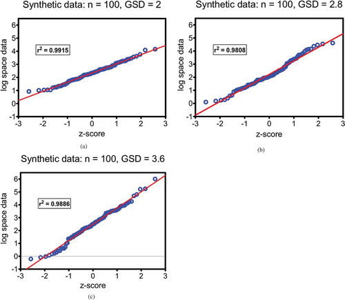
Figure 2. a, b: Comparisons of ICC calculation methods of perfectly balanced data with respect to different data parameters of GSD and target ICC. Each dataset has 100 subjects; a) comparisons for two measurements per subject and b) comparisons for 10 measurements per subject. Differences between Figure 2a and 2b are due to the number repeat measures and not due to the method of calculation. Each test was performed three times.

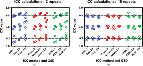
Recall that these were balanced data with the same number of repeat values and no missing values. The next step was to randomly remove 10% of the values to determine if such missing values would upset the calculations. Figures 3a and 3b show these results across all tested methods and parameters.

Again, the results are equivocal with respect to calculation method. The only important factor in reducing variability is to increase the number of repeated measures. The results of part 1 indicate that a relative large number of samples (n = 100) has sufficient power to overwhelm the effect of statistical variability with respect to the different methods of ICC calculation.

Calculation results of ICCs — part 2

The results of part 1 left the question as to what happens in more sparse datasets. Often preliminary experiments with human subjects only have about 10 or 20 subjects, and so perhaps the more sophisticated approaches could be valuable. Because the target ICC, the number of repeats, and the GSD do not appear to affect the outcomes with respect to calculation method, median parameters of target ICC = 0.5, repeats k = 3, and GSD = 2.8 were selected as constants, and only the number of sample subjects were varied as n = 10, 20, 50, and 100; the latter (n = 100) was used for continuity.

The combined effects of calculation method and number of samples are essentially equivocal. Although overall variability increases as the number of samples is reduced, the dotted lines used to guide the eye indicate only a small potential improvement in scatter of the ANOVA and REML estimates over the variance calculations. This is not a compelling reason to affect the choice of method used to calculate ICC.

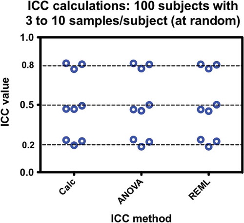
Calculation results of ICCs — part 3

The final issue that might affect the outcome of ICC estimates is highly unbalanced data. To test this, datasets were created that had target values of ICC = 0.2, 0.5, and 0.8, with values randomly selected from repeats of 3 to 10 samples per subject. The remaining parameters were held constant at n = 100, GSD = 2.8. The initial thought was that variance calculations and ANOVA might be adversely affected by such severely unbalanced datasets and that REML might be a superior method. As seen in (Figure 5), once again the method of calculation is shown to be irrelevant.

Figure 3. a, b: Comparisons of ICC calculation methods of data missing 10% of the values at random with respect to different data parameters of GSD and target ICC. Each dataset has 100 subjects; a) comparisons for two measurements per subject and b) comparisons for 10 measurements per subject. Differences between Figure 3a and 3b are due to the number repeat measures and not due to the method of calculation. Furthermore, missing at random values do not affect the character of the comparisons of the ICCs. Each test was performed three times.

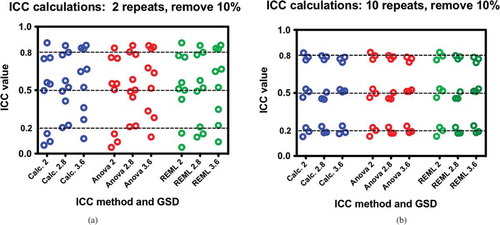
Figure 4. Comparisons of ICC calculation methods with respect to the number of subjects. All data sets have three measures per subject with10% of data removed at random. Scatter increases as number of samples decreases; however, the method of calculation does not affect the results. Each test was performed three times.

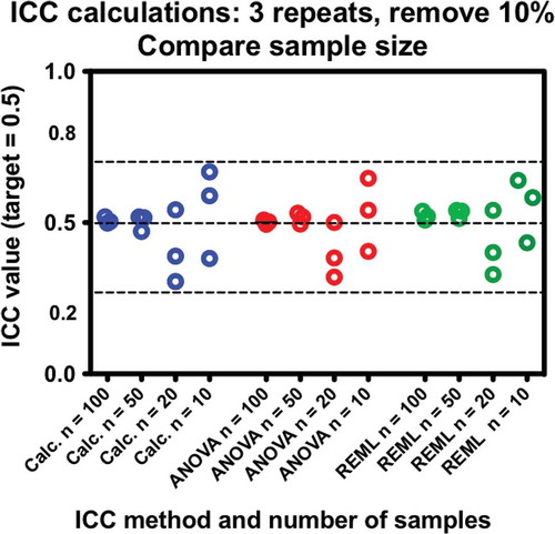
Figure 5. Comparisons of ICC calculation methods with respect to severely unbalanced data. At random, 100 subjects have anywhere from 3 to 10 measurements each for datasets targeted for 0.2, 0.5, and 0.8 ICC values. The method of calculation does not affect the results. Each test was performed three times.

Summary of calculation methods

This part of the review showed how to construct hypothetical data that are lognormally distributed between subjects for specific GM and GSD and simultaneously achieve repeat measures with targeted ICC based upon Excel functionality. This is a valuable tool for testing statistical evaluations that would be subsequently applied to real-world data where the summary statistics are not known. In addition, once GM, GSD, and ICC are estimated from a real-world dataset, the procedures shown here may be used to build bigger more detailed datasets for modeling purposes or for evaluating sparse metadata parameters.

The more important part of this section, however, is the test of the hypothesis that more complex ICC calculations are less prone to variability from perturbations in real-world data. This could not be confirmed; there were no discernible differences found among variance calculations, ANOVA table calculations, and REML estimates with respect to stability of ICC assessments. In fact, the main conclusion from this work confirms the concept (Giraudeau and Mary 2001) that the precision of ICC estimates is most affected by the particular distribution of the sample, the number of repeat measures, and the total number of samples, as illustrated in the figures. This is shown in the “left to right” patterns in Figures 2, 3, 4, and 5, which reflect the repeated datasets; that is, the heights track across demonstrating that the ICC calculation depends upon the character of the data, not the calculation method.

From an operational standpoint, the major advantages of using the REML estimator method as implemented in SAS (or other similar software) is that it seamlessly incorporates samples that have only a single measurement and large datasets that are difficult to assess in a limited spreadsheet environment. Moreover, the mixed model approach allows more flexibility in dealing with more complicated (multilevel) datasets. In contrast, the variance and ANOVA calculations require removal of samples that have only a single measure from the dataset and thus invoke extra effort in manual data curation. Further, spreadsheet analyses have practical limitations as to sample size.

The ultimate value of this section was to demonstrate practical means for estimating ICC and that it is sufficient to use whichever of the three ICC calculation methods is most convenient. Normally, this choice is driven by the structure and complexity of the dataset and which format the data happen to be in when they reach the researcher. For example, if the dataset is already imbedded into a SAS program format, and proc mixed has already been implemented to assess a complex model, then adding a few lines of code to calculate ICC from the covariance analysis is indicated. However, if the investigator has a rectangular array of measurements in a spreadsheet, then 1-way ANOVA or variance calculation methods would be simpler to invoke.

Conclusions

This review demonstrates the history of implementing repeat measures into study designs. The primary value is to explain the rationale for incorporating repeat measures designs into biomonitoring, or other related environmental studies, and to provide some mathematical tools to calculate the intra-class correlation coefficient.

Acknowledgments

The authors are grateful for expert advice from Jon Sobus, Seth Newton, Johnsie Lang, and Adam Biales from U.S. EPA. J. Pleil and W. Funk are particularly grateful for the mentorship of our PhD advisor, Prof. Stephen Rappaport, a pioneer in mathematical modeling of occupational and environmental exposure measurement, now at University of California, Berkeley. This article was reviewed in accordance with the policies of the National Exposure Research Laboratory and U.S. Environmental Protection Agency and approved for publication. Mention of trade names or commercial products does not constitute endorsement or recommendation for use.

APPENDIX 1

What is ICC?

ICC is a single, non-dimensional parameter that characterizes one small part of a complex data set with repeat measures. The ICC needs to be carefully used and interpreted under the constraints of the experiment and within the overall distribution of the measured data. ICC tells a simple story: How much of the variance in one’s measurements is coming from true differences among the samples (or the human subjects) and how much is coming from other changes (e.g. time, sample collection, analysis, or random error).

As a simple example, consider that one has 10 bottles of wine and wants an objective quality rating. One could just taste each one and write down a subjective score. This makes a few assumptions: one is completely objective over time, one could actually tell the difference among the bottles of wine, and a previous bottle doesn’t bias one for the current one. None of these may not be true! The use of repeat measures and ICC resolves these issues.

Suppose instead that one covers all the labels and just numbers the bottles at random from 1 to 10. Then, one tastes each one anonymously and scores them on some scale relative as to how much one likes them. With the help of a friend to track the numbers, one then tastes each bottle again in some random order without knowing which one is which and scores them again; this could be repeated as many times as one likes. The closer the repeat measures are for each bottle, the better is ones ability to taste wines. This is used to calculate the “within-bottle” variance. The range of all the measurements is used to calculate the “total” variance, which is the sum of the “between-bottle” and “within-bottle” variance. The ICC is defined as the ratio of “between-bottle” variance divided by the “total” variance and can take a value between 0 and 1.

Suppose that there are really big true differences among the bottles of wine and that ones measured ICC is fairly large, say 0.8. This means that one is a good discriminator of wine. Suppose, however, the same wines result in a small ICC, say 0.2. This means one is not that good at telling wines apart and the scores are mostly random.

Now, suppose that all of the wines are actually really, really good; now, a low ICC does not indict tasting prowess because all of the scores, regardless of bottle, should be relatively high and therefore close. If one is terrible at evaluating wine, one could get a higher ICC, maybe around 0.5, because the measures would be mostly random and so half of the variance would be ascribed to the bottles and the other half to one’s judgment prowess.

Important:

ICC depends not only on how good the measurements are but also on how much range there is among the units measured. This is a critical concern when interpreting ICC data; one has to understand the range of the data as well as the precision of the measurements.

References

- Alfano, C. M. 2012. Physical activity, biomarkers, and disease outcomes in cancer survivors: A systematic review. Journal of the National Cancer Institute 104:815–40. doi:10.1093/jnci/djs207.
- Amann, A., B. de Lacy Costello, W. Miekisch, J. Schubert, B. Buszewski, J. D. Pleil, N. Ratcliffe, and T. H. Risby. 2014. The human volatilome: Volatile organic compounds (VOCs) in exhaled breath, skin emanations, urine, feces and saliva. Journal of Breath Research 8:034001. doi:10.1088/1752-7155/8/3/034001.
- Angrish, M. M., J. D. Pleil, M. A. Stiegel, M. C. Madden, V. C. Moser, and D. W. Herr. 2016. Taxonomic applicability of inflammatory cytokines in adverse outcome pathway (AOP) development. Journal of Toxicology and Environmental Health A 79:184–96. doi:10.1080/15287394.2016.1138923.
- Aylward, L. L., C. R. Kirman, J. L. Adgate, L. M. McKenzie, and S. M. Hays. 2012. Interpreting variability in population biomonitoring data: Role of elimination kinetics. Journal of Exposure Science and Environmental Epidemiology 22:398–408. doi:10.1038/jes.2012.35.
- Baker, D. B., and M. J. Nieuwenhuijsen, ed. 2008. Environmental epidemiology: Study methods and application. Oxford: Oxford University Press.
- Ballard-Barbash, R., C. M. Friedenreich, K. S. Courneya, S. M. Siddiqi, A. McTiernan, and C. M. Alfano. 2012. Physical activity, biomarkers, and disease outcomes in cancer survivors: A systematic review. Journal of the National Cancer Institute 104:815–40. doi:10.1093/jnci/djs207.
- Bartko, J. J. 1976. On various intraclass correlation reliability coefficients. Psychological Bulletin 83:762. doi:10.1037/0033-2909.83.5.762.
- Bartlett, M. S. 1937. Properties of sufficiency and statistical tests. Proceedings of the Royal Society of London 160: 268–82.
- Bell, B. A., M. Ene, W. Smiley, and J. A. Schoeneberger. 2013. A multilevel model primer using SAS PROC MIXED. SAS Global Forum. University of South Carolina College of Education, Columbia, SC. http://support.sas.com/resources/papers/proceedings13/433-2013.pdf.
- Boffetta, P., N. Jourenkova, and P. Gustavsson. 1997. Cancer risk from occupational and environmental exposure to polycyclic aromatic hydrocarbons. Cancer Causes & Control 8:444–72. doi:10.1023/A:1018465507029.
- Bonvallot, N., M. Tremblay-Franco, C. Chevrier, C. Canlet, L. Debrauwer, J. P. Cravedi, and S. Cordier. 2014. Potential input from metabolomics for exploring and understanding the links between environment and health. Journal of Toxicology and Environmental Health B 17:21–44. doi:10.1080/10937404.2013.860318.
- Breit, M., C. Baumgartner, M. Netzer, and K. M. Weinberger. 2016. Clinical bioinformatics for biomarker discovery in targeted metabolomics. In Application of Clinical Bioinformatics, ed. X. Wang, C. Baumgartner, D. Shields, HW Deng, J. Beckmann, 213–40. Dordrecht: Springer.
- Brown, J. R., and J. L. Thornton. 1957. Percivall Pott (1714-1788) and chimney sweepers’ cancer of the scrotum. British Journal of Industrial Medicine 14:68.
- Centers for Disease Control and Prevention (CDC), 2009. Fourth national report on human exposure to environmental chemicals, 1600 Clifton Rd Atlanta, GA 30333 http://www.cdc.gov/exposurereport/
- Cherrie, J. W. 2003. Commentary: The beginning of the science underpinning occupational hygiene. Annals of Occupational Hygiene 47:179–85.
- Cole, D. C., J. Eyles, and B. L. Gibson. 1998. Indicators of human health in ecosystems: What do we measure? Science of the Total Environment 224:201–13.
- Corbeil, R. R., and S. R. Searle. 1976. Restricted maximum likelihood (REML) estimation of variance components in the mixed model. Technometrics 18:31–38. doi:10.2307/1267913.
- Cosselman, K. E., A. Navas-Acien, and J. D. Kaufman. 2015. Environmental factors in cardiovascular disease. Nature Reviews Cardiology 12:627. doi:10.1038/nrcardio.2015.152.
- Daughton, C. G. 2012. Using biomarkers in sewage to monitor community-wide human health: Isoprostanes as conceptual prototype. Science of the Total Environment 424:16–38. doi:10.1016/j.scitotenv.2012.02.038.
- Delfino, R. J. 2002. Epidemiologic evidence for asthma and exposure to air toxics: Linkages between occupational, indoor, and community air pollution research. Environmental Health Perspectives 110(Suppl 4):573.
- Diamond, G. L., N. P. Skoulis, A. R. Jeffcoat, and J. F. Nash. 2017. A physiologically based pharmacokinetic model for the broad-spectrum antimicrobial zinc pyrithione: I. Development and verification. Journal of Toxicology and Environmental Health A 80:69–90. doi:10.1080/15287394.2016.1245123.
- Egeghy, P. P., R. Tornero-Velez, and S. M. Rappaport. 2000. Environmental and biological monitoring of benzene during self-service automobile refueling. Environmental Health Perspectives 108:1195–202.
- Epa, U. S. 2012. Biomonitoring - an exposure science tool for exposure and risk assessment. Washington, DC: U.S. Environmental Protection Agency. EPA/600/R-12/039 (NTIS PB2012-112321).
- Etzel, R. A. 2003. How environmental exposures influence the development and exacerbation of asthma. Pediatrics 112(Supplement 1):233–39.
- Fisher, R. A. 1918. The correlation between relatives on the supposition of mendelian inheritance. Philosophical Transactions of the Royal Society of Edinburgh 52:399–433. doi:10.1017/S0080456800012163.
- Fisher, R. A. 1921. On the “Probable Error” of a coefficient of correlation deduced from a small sample. Metron 1:3–32.
- Fisher, R. A. 1925. Statistical methods for research workers, Oliver and Boyd Ltd., Edinburgh. 5th. is available online: http://www.haghish.com/resources/materials/Statistical_Methods_for_Research_Workers.pdf.
- Giraudeau, B., and J. Y. Mary. 2001. Planning a reproducibility study: How many subjects and how many replicates per subject for an expected width of the 95 per cent confidence interval of the intraclass correlation coefficient. Statistics in Medicine 20:3205–14.
- Goldstein, H. 1986. Multilevel mixed linear model analysis using iterative generalized least squares. Biometrika 73:43–56. doi:10.1093/biomet/73.1.43.
- Gordon, J. N., A. Taylor, and P. N. Bennett. 2002. Lead poisoning: Case studies. British Journal of Clinical Pharmacology 53:451–58.
- Gulliford, M. C., O. C. Ukoumunne, and S. Chinn. 1999. Components of variance and intraclass correlations for the design of community-based surveys and intervention studies: Data from the Health Survey for England 1994. American Journal of Epidemiology 149:876–83.
- Hall, J. E. 2015. Guyton and hall textbook of medical physiology e-book. Elsevier Health Sciences. eBook. 13th edition (Online), Saunders. ISBN:9780323389303.
- Ismail, A. A., K. Wang, J. R. Olson, M. R. Bonner, O. Hendy, G. Abdel Rasoul, and D. S. Rohlman. 2017. The impact of repeated organophosphorus pesticide exposure on biomarkers and neurobehavioral outcomes among adolescent pesticide applicators. Journal of Toxicology and Environmental Health A 80:542–55. doi:10.1080/15287394.2017.1362612.
- Johnson, C. H., and F. J. Gonzalez. 2012. Challenges and opportunities of metabolomics. Journal of Cellular Physiology 227:2975–81. doi:10.1002/jcp.24002.
- Kessler, R., and R. E. Glasgow. 2011. A proposal to speed translation of healthcare research into practice: Dramatic change is needed. American Journal of Preventative Medicine 40:637–44. doi:10.1016/j.amepre.2011.02.023.
- Koo, T. K., and M. Y. Li. 2016. A guideline of selecting and reporting intraclass correlation coefficients for reliability research. Journal of Chiropractic Medicine 15:155–63. doi:10.1016/j.jcm.2016.02.012.
- Kromhout, H., Y. Oostendorp, D. Heederik, and J. S. Boleij. 1987. Agreement between qualitative exposure estimates and quantitative exposure measurements. American Journal of Industrial Medicine 12:551–62.
- Kromhout, H., E. Symanski, and S. M. Rappaport. 1993. A comprehensive evaluation of within-and between-worker components of occupational exposure to chemical agents. Annals of Occupational Hygiene 37:253–70.
- LaKind, J. S., L. G. Anthony, and M. Goodman. 2017. Review of reviews on exposures to synthetic organic chemicals and children’s neurodevelopment: Methodological and interpretation challenges. Journal of Toxicology and Environmental Health A 20:390–422. doi:10.1080/10937404.2017.1370847.
- Landis, J. R., T. S. King, J. W. Choi, V. M. Chinchilli, and G. G. Koch. 2011. Measures of agreement and concordance with clinical research applications. Statistics in Biopharmaceutical Research 3:185–209. doi:10.1198/sbr.2011.10019.
- Lianidou, E. S., and A. Markou. 2011. Circulating tumor cells in breast cancer: Detection systems, molecular characterization, and future challenges. Clinical Chemistry 57:1242–55. doi:10.1373/clinchem.2011.165068.
- Lin, Y. S., L. L. Kupper, and S. M. Rappaport. 2005. Air samples versus biomarkers for epidemiology. Occupation and Environmental Medicine 62:750–60. doi:10.1136/oem.2004.013102.
- Lyles, R. H., L. L. Kupper, and S. M. Rappaport. 1997. A lognormal distribution-based exposure assessment method for unbalanced data. Annals of Occupational Hygiene 41:63–76. doi:10.1016/S0003-4878(96)00020-8.
- McGraw, K. O., and S. P. Wong. 1996. Forming inferences about some intraclass correlation coefficients. Psychological Methods 1:30–46. doi:10.1037/1082-989X.1.1.30.
- Mehan, M. R., R. Ostroff, S. K. Wilcox, F. Steele, D. Schneider, T. C. Jarvis, G. S. Baird, L. Gold, and N. Janjic. 2013. Highly multiplexed proteomic platform for biomarker discovery, diagnostics, and therapeutics. In Complement Therapeutics, ed. J. D. Lambris, V. M. Holers, D. Ricklin, 283–300. Boston, MA: Springer.
- Metcalf, S. W., and K. G. Orloff. 2004. Biomarkers of exposure in community settings. Journal of Toxicology and Environmental Health A 67:715–26. doi:10.1080/15287390490428198.
- Moons, K. G., J. A. de Groot, K. Linnet, J. B. Reitsma, and P. M. Bossuyt. 2012. Quantifying the added value of a diagnostic test or marker. Clinical Chemistry 58:1408–17. doi:10.1373/clinchem.2012.182550.
- Müller, R., and P. Büttner. 1994. A critical discussion of intraclass correlation coefficients. Statistics in Medicine 13:2465–76.
- National Institutes of Environmental Health (NIEHS). 2012. “Biomarkers.” http://www.niehs.nih.gov/health/topics/science/biomarkers/
- National Research Council (NRC). 2006. Human biomonitoring for environmental chemicals. Washington, DC: The National Academies Press.
- Oldham, P. D., and S. A. Roach. 1952. A sampling procedure for measuring industrial dust exposure. British Journal of Industrial Medicine 9:112–19.
- Orchard, S., P. A. Binz, C. Borchers, M. K. Gilson, A. R. Jones, G. Nicola, J. A. Vizcaino, E. W. Deutsch, and H. Hermjakob. 2012. Ten years of standardizing proteomic data: A report on the HUPO‐PSI spring workshop. Proteomics 12:2767–72. doi:10.1002/pmic.201270126.
- Pierce, K. M., J. C. Hoggard, R. E. Mohler, and R. E. Synovec. 2008. Recent advancements in comprehensive two-dimensional separations with chemometrics. Journal of Chromatography A 1184:341–52. doi:10.1016/j.chroma.2007.07.059.
- Pleil, J. D. 2009. Influence of systems biology response and environmental exposure level on between-subject variability in breath and blood biomarkers. Biomarkers 14:560–71. doi:10.3109/13547500903186460.
- Pleil, J. D. 2012. Categorizing biomarkers of the human exposome and developing metrics for assessing environmental sustainability. Journal of Toxicology and Environmental Health B 15:264–80. doi:10.1080/10937404.2012.672148.
- Pleil, J. D. 2015. Understanding new “exploratory” biomarker data: A first look at observed concentrations and associated detection limits. Biomarkers 20:168–69. doi:10.3109/1354750X.2015.1040841.
- Pleil, J. D. 2016a. Breath biomarkers in toxicology. Archives of Toxicology 90:2669–82. doi:10.1007/s00204-016-1817-5.
- Pleil, J. D. 2016b. QQ-plots for assessing distributions of biomarker measurements and generating defensible summary statistics. Journal of Breath Research 10:035001. doi:10.1088/1752-7155/10/3/035001.
- Pleil, J. D. 2016c. Imputing defensible values for left-censored ‘below level of quantitation’ (LoQ) biomarker measurements. Journal of Breath Research 10:045001. doi:10.1088/1752-7155/10/4/045001.
- Pleil, J. D., J. D. Beauchamp, and W. Miekisch. 2017. Cellular respiration, metabolomics and the search for illicit drug biomarkers in breath: Report from PittCon 2017. Journal of Breath Research 11:039001. doi:10.1088/1752-7163/aa7174.
- Pleil, J. D., and K. K. Isaacs. 2016. High-resolution mass spectrometry: Basic principles for using exact mass and mass defect for discovery analysis of organic molecules in blood, breath, urine and environmental media. Journal of Breath Research 10:012001. doi:10.1088/1752-7155/10/1/012001.
- Pleil, J. D., and L. S. Sheldon. 2011. Adapting concepts from systems biology to develop systems exposure event networks for exposure science research. Biomarkers 16:99–105. doi:10.3109/1354750X.2010.541565.
- Pleil, J. D., and J. R. Sobus. 2013. Estimating lifetime risk from spot biomarker data and intra-class correlation coefficients (ICC). Journal of Toxicology and Environmental Health A 76:747–66. doi:10.1080/15287394.2013.821394.
- Pleil, J. D., and J. R. Sobus. 2016. Estimating central tendency from a single spot measure: A closed-form solution for lognormally distributed biomarker data for risk assessment at the individual level. Journal of Toxicology and Environmental Health A 79:837–47. doi:10.1080/15287394.2016.1193108.
- Pleil, J. D., J. R. Sobus, M. A. Stiegel, D. Hu, K. D. Oliver, C. Olenick, M. Strynar, M. Clark, M. C. Madden, and W. E. Funk. 2014. Estimating common parameters of lognormally distributed environmental and biomonitoring data: Harmonizing disparate statistics from publications. Journal of Toxicology and Environmental Health B 17 341–68. doi:10.1080/10937404.2014.956854.
- Pleil, J. D., M. A. Stiegel, M. C. Madden, and J. R. Sobus. 2011c. Heat map visualization of complex environmental and biomarker measurements. Chemosphere 84:716–23. doi:10.1016/j.chemosphere.2011.03.017.
- Pleil, J. D., M. A. Stiegel, and J. R. Sobus. 2011a. Breath biomarkers in environmental health science: Exploring patterns in the human exposome. Journal of Breath Research 5:046005. doi:10.1088/1752-7155/5/4/046005.
- Pleil, J. D., M. A. Stiegel, J. R. Sobus, W. Liu, and M. C. Madden. 2011b. Observing the human exposome as reflected in breath biomarkers: Heat map data interpretation for environmental and intelligence research. Journal of Breath Research 5:037104. doi:10.1088/1752-7155/5/3/037104.
- Pleil, J. D., M. Williams, and J. R. Sobus. 2012. Chemical Safety for Sustainability (CSS): Biomonitoring in vivo data for distinguishing among adverse, adaptive, and random responses from in vitro toxicology. Toxicology Letters 215:201–07. doi:10.1016/j.toxlet.2012.10.011.
- Polichetti, G., S. Cocco, A. Spinali, V. Trimarco, and A. Nunziata. 2009. Effects of particulate matter (PM10, PM2. 5 and PM1) on the cardiovascular system. Toxicology 261:1–8. doi:10.1016/j.tox.2009.04.035.
- Rappaport, S. M. 1984. The rules of the game: An analysis of OSHA’s enforcement strategy. American Journal of Industrial Medicine 6:291–303.
- Rappaport, S. M. 1991. Assessment of long-term exposures to toxic substances in air. Annals of Occupational Hygiene 35:61–121.
- Rappaport, S. M., and L. L. Kupper. 2008. Quantitative exposure assessment. El Cerrito, CA: S.M. Rappaport.
- Rappaport, S. M., R. H. Lyles, and L. L. Kupper. 1995. An exposure assessment strategy accounting for within and between workers sources of variability. Annals of Occupational Hygiene 39:469–95.
- Rappaport, S. M., and M. T. Smith. 2010. Epidemiology: Environment and disease risk. Science 33:460–61. doi:10.1126/science.1192603.
- Rappaport, S. M., R. C. Spear, and S. Selvin. 1988. The influence of exposure variability on dose-response relationships in Inhaled Particles VI, Proceedings of an International Symposium and Workshop on Lung Dosimetry, British Occupational Hygiene Society, pp. 529–37.
- Rubino, F. M., M. Pitton, D. Di Fabio, and A. Colombi. 2009. Toward an “omic” physiopathology of reactive chemicals: Thirty years of mass spectrometric study of the protein adducts with endogenous and xenobiotic compounds. Mass Spectrometry Reviews 28:725–84. doi:10.1002/mas.20207.
- Ruiz, I., M. Sprowls, Y. Deng, D. Kulick, H. Destaillats, and E. S. Forzani. 2018. Assessing metabolic rate and indoor air quality with passive environmental sensors. Journal of Breath Research 12:036012. doi:10.1088/1752-7163/aaaec9.
- Sexton, K., and A. D. Ryan. 2012. Using exposure biomarkers in children to compare between-child and within-child variance and calculate correlations among siblings for multiple environmental chemicals. Journal of Exposure Science and Environmental Epidemiology 22:16–23. doi:10.1038/jes.2011.30.
- Shek, D. T., and C. Ma. 2011. Longitudinal data analyses using linear mixed models in SPSS: Concepts, procedures and illustrations. The Scientific World Journal 11:42–76. doi:10.1100/tsw.2011.2.
- Sherwood, R. J., and M. Lippmann. 1997. Historical perspectives: Realization, development, and first applications of the personal air sampler. Applied Occupational and Environmental Hygiene 12:229–34. doi:10.1080/1047322X.1997.10389495.
- Shrout, P. E., and J. L. Fleiss. 1979. Intraclass correlations: Uses in assessing rater reliability. Psychological Bulletin 86:420. doi:10.1037/0033-2909.86.2.420.
- Silva, S. S., C. Lopes, A. L. Teixeira, M. C. de Sousa, and R. Medeiros. 2015. Forensic miRNA: Potential biomarker for body fluids? Forensic Science International: Genetics 14:1–10. doi:10.1016/j.fsigen.2014.09.002.
- Singer, J. D. 1998. Using SAS PROC MIXED to fit multilevel models, hierarchical models, and individual growth models. Journal of Educational and Behavioral Statistics 23:323–55. doi:10.3102/10769986023004323.
- Sobus, J. R., R. S. Dewoskin, Y. M. Tan, J. D. Pleil, M. B. Phillips, B. J. George, K. Y. Christensen, D. M. Schreinemachers, M. A. Williams, E. A. Cohen-Hubal, and S. W. Edwards. 2015. Uses of NHANES biomarker data for chemical risk assessment: Trends, challenges and opportunities. Environmental Health Perspectives 123:919–27. doi:10.1289/ehp.1409177.
- Sobus, J. R., M. D. McClean, R. F. Herrick, S. Waidyanatha, L. A. Nylander-French, L. L. Kupper, and S. M. Rappaport. 2009. Comparing urinary biomarkers of airborne and dermal exposure to polycyclic aromatic compounds in asphalt-exposed workers. Annals of Occupational Hygiene 53:561–71. doi:10.1093/annhyg/mep042.
- Sobus, J. R., M. K. Morgan, J. D. Pleil, and D. B. Barr. 2010b. Biomonitoring: Current tools and approaches for assessing human exposure to pesticides, Chap. 45: Hayes handbook of pesticide toxicology, Elsevier Ltd. Oxford, UK, ed. R. Krieger
- Sobus, J. R., J. D. Pleil, M. D. McClean, R. F. Herrick, and S. M. Rappaport. 2010a. Biomarker variance component estimation for exposure surrogate selection and toxicokinetic inference. Toxicology Letters 199:247–53. doi:10.1016/j.toxlet.2010.09.006.
- Stiegel, M. A., J. D. Pleil, J. R. Sobus, T. Stevens, and M. C. Madden. 2017. Linking physiological parameters to perturbations in the human exposome: Environmental exposures modify blood pressure and lung function via inflammatory cytokine pathway. Journal of Toxicology and Environmental Health, Part A 80:485–501. doi:10.1080/15287394.2017.1330578.
- Stigler, S. M. 1990. The history of statistics. The measurement of uncertainty before 1900. Belknap Press World: Cambridge, MA.
- Tan, Y. M., J. R. Sobus, D. Chang, R. Tornero-Velez, M. Goldsmith, J. D. Pleil, and C. Dary. 2012. Reconstructing human exposures using biomarkers and other “clues”. Journal of Toxicology and Environmental Health, Part B 15:22–38. doi:10.1080/10937404.2012.632360.
- Tinsley, H. E., and D. J. Weiss. 1975. Interrater reliability and agreement of subjective judgments. Journal of Counseling Psychology 22:358. doi:10.1037/h0076640.
- Tremaroli, V., and F. Bäckhed. 2012. Functional interactions between the gut microbiota and host metabolism. Nature 489:242–49. doi:10.1038/nature11552.
- Tsai, -S.-S., C.-Y. Tsai, and C.-Y. Yang. 2018. Fine particulate air pollution associated with risk of hospital admissions for hypertension in a tropical city, Kaohsiung, Taiwan. Journal of Toxicology and Environmental Health A 81:567–75. doi:10.1080/15287394.2018.1460788.
- Wallace, M. A., T. M. Kormos, and J. D. Pleil. 2016. Blood-borne biomarkers and bioindicators for linking exposure to health effects in environmental health science. Journal of Toxicology and Environmental Health B 19:380–409. doi:10.1080/10937404.2016.1215772.
- Walton, W. H., and J. H. Vincent. 1998. Aerosol instrumentation in occupational hygiene: An historical perspective. Aerosol Science and Technology 28:417–38. doi:10.1080/02786829808965535.
- Wang, C. S., B. S. Yandell, and J. J. Rutledge. 1992. The dilemma of negative analysis of variance estimators of intraclass correlation. Theoretical and Applied Genetics 85:79–88. doi:10.1007/BF00223848.
- Wang, L., D. Du, D. Lu, C. T. Lin, J. N. Smith, C. Timchalk, F. Liu, J. Wang, and Y. Lin. 2011. Enzyme-linked immunosorbent assay for detection of organophosphorylated butyrylcholinesterase: A biomarker of exposure to organophosphate agents. Analytica Chimica Acta 693:1–6. doi:10.1016/j.aca.2011.03.013.
- Weaver, M. A., L. L. Kupper, D. Taylor, H. Kromhout, P. Susi, and S. M. Rappaport. 2001. Simultaneous assessment of occupational exposures from multiple worker groups. Annals of Occupational. Hygiene 45:525–42. doi:10.1016/S0003-4878(01)00014-X.
- Weir, J. P. 2005. Quantifying test-retest reliability using the intraclass correlation coefficient and the SEM. Journal of Strength and Conditioning Research 19:231–40. doi:10.1519/15184.1.
- Wild, C. P. 2005. Complementing the genome with an “exposome”: The outstanding challenge of environmental exposure measurement in molecular epidemiology. Cancer Epidemiology, Biomarkers, & Prevention 14:1847–50. doi:10.1158/1055-9965.EPI-05-0456.
- Zuurman, L., A. E. Ippel, E. Moin, and J. Van Gerven. 2009. Biomarkers for the effects of cannabis and THC in healthy volunteers. British Journal of Clinical Pharmacology 67:5–21. doi:10.1111/j.1365-2125.2008.03329.x.