Effects of improved spatial and temporal modeling of on-road vehicle emissions

Abstract

Numerous emission and air quality modeling studies have suggested the need to accurately characterize the spatial and temporal variations in on-road vehicle emissions. The purpose of this study was to quantify the impact that using detailed traffic activity data has on emission estimates used to model air quality impacts. The on-road vehicle emissions are estimated by multiplying the vehicle miles traveled (VMT) by the fleet-average emission factors determined by road link and hour of day. Changes in the fraction of VMT from heavy-duty diesel vehicles (HDDVs) can have a significant impact on estimated fleet-average emissions because the emission factors for HDDV nitrogen oxides (NO_x) and particulate matter (PM) are much higher than those for light-duty gas vehicles (LDGVs). Through detailed road link-level on-road vehicle emission modeling, this work investigated two scenarios for better characterizing mobile source emissions: (1) improved spatial and temporal variation of vehicle type fractions, and (2) use of Motor Vehicle Emission Simulator (MOVES2010) instead of MOBILE6 exhaust emission factors. Emissions were estimated for the Detroit and Atlanta metropolitan areas for summer and winter episodes. The VMT mix scenario demonstrated the importance of better characterizing HDDV activity by time of day, day of week, and road type. More HDDV activity occurs on restricted access road types on weekdays and at nonpeak times, compared to light-duty vehicles, resulting in 5–15% higher NO_x and PM emission rates during the weekdays and 15–40% lower rates on weekend days. Use of MOVES2010 exhaust emission factors resulted in increases of more than 50% in NO_x and PM for both HDDVs and LDGVs, relative to MOBILE6. Because LDGV PM emissions have been shown to increase with lower temperatures, the most dramatic increase from MOBILE6 to MOVES2010 emission rates occurred for PM_2.5 from LDGVs that increased 500% during colder wintertime conditions found in Detroit, the northernmost city modeled.

Implications:

Air quality model performance relies partly on on-road mobile source emission inventories accurately allocated, both spatially and temporally. This work demonstrates the importance of characterizing the mix of heavy-duty diesel versus light-duty gasoline vehicle activity on an hourly basis on weekdays and weekends by road type. Incorporating detailed activity data increases weekday average NO_x and PM emissions 5–15%, with early morning hour emission increases approaching 100%, compared to using one average vehicle activity mix. Application of the methodologies described in this paper will improve the accuracy of on-road emission inventories in the understanding of ozone photochemistry and PM formation.

Introduction

Most of the on-road emission inventories historically have been prepared by using U.S. Environmental Protection Agency's (EPA's) regulatory emission factor model, combined with estimates of vehicle miles traveled (VMT) from local transportation data, to estimate average annual (or seasonal) daily emissions. The daily emissions are then allocated to hours of the day and days of the week for the air quality modeling episode using temporal profiles developed by EPA (EPA, 2012c). The hourly exhaust emissions are then allocated to model grid cells using spatial allocation surrogates based on the location of major roadways, also developed by EPA (EPA, 2012d). These emission estimates may be reasonable for large regional modeling domains over seasonal or longer time periods, but for fine-scale urban air quality modeling, emission estimates developed in this way can be significantly inaccurate.

There are a number of factors that contribute to significant inaccuracies in on-road vehicle emission inventories developed using this approach. First, the temporal profiles used to disaggregate daily emissions to hourly emissions have been developed from VMT activity data that do not reflect the temporal distribution of emissions resulting from the travel patterns of heavy- and light-duty vehicles and diurnal meteorology. On a typical weekday in summer, VMT peaks in the morning and afternoon commute hours. Vehicle emissions in summer, however, are significantly influenced by meteorological factors. For example, total organic gas (TOG) emissions in most areas are much higher in summer afternoon commute hours than morning commute hours because of higher temperatures affecting both exhaust and evaporative emissions. Second, the fractions of VMT from light-duty gasoline vehicles (LDGVs; cars and trucks) and heavy-duty diesel vehicles (HDDVs) are assumed to be constant over the hours of the day and the days of the week, and often constant across roadway types as well. However, it has been shown that the fraction of VMT from trucks is highest on interstates and freeways, and less on collectors and smaller roads (Lindhjem and Shepard, 2007). In addition, the constituent fractions of VMT by vehicle class (referred to as VMT mix) vary significantly over the hours of the day (e.g., many HDDV drivers may avoid peak hours when relatively higher LDGV traffic occurs) and over the days of the week. Third, a simplistic assumption is made of setting speeds on all road “links” (individual roadway segments) of the same functional classification to the same average speed. In fact, link speeds can vary significantly across different roads of the same type and across hours of the day, depending on the level of congestion, particularly in urban areas. Moreover, actual speeds vary on the same roadway depending on the level of congestion, and those changes in speed can have a significant effect on spatial and temporal emissions rates (Bai et al., 2007).

Two additional factors that can contribute to emissions inaccuracy are the lack of use of local inputs and meteorology. Key local inputs for on-road emission modeling that affect emission rates are vehicle age distributions (obtained from registration records), vehicle Inspection and Maintenance implementation, and fuel control programs. Over the last 30 years, emissions standards for both cars and trucks have been dramatically reduced (EPA, 1997, 2007). As a result, a fleet that is older or newer than a default national average can have significantly higher or lower emissions, respectively. Evaporative TOG emissions are reduced where local fuel control programs reduce summer gasoline vapor pressure, and CO emissions are lower in areas where oxygenates are added to fuels. Regarding meteorology, TOG exhaust emissions depend on temperature and humidity as expressed through the heat index, NO_x emissions depend on temperature and humidity, and particulate matter (PM) emissions from LDGVs increase exponentially at lower temperatures (EPA, 2008).

Numerous emissions and air quality modeling studies in the past decade or so have pointed out how the above inaccuracies with regard to temporal emissions can affect air quality modeling. One important example is in the differences between weekday and weekend (WD/WE) emissions and subsequent air quality impacts. The WD/WE effect was first observed in Los Angeles, where monitoring data showed higher ozone on weekends than weekdays (Blanchard and Tanenbaum, 2003; Elkus and Wilson, 1976; Fujita et al., 2003; Lawson, 2003; Levitt and Chock, 1976). Air quality modeling and data analysis studies for Los Angeles showed that this was the result of lower NO_x emissions and changes in timing of NO_x emissions on weekends in large part because higher NO_x-emitting HDDV traffic is significantly lower on weekend days, combined with changes in volatile organic compound (VOC) emissions, which resulted in increased VOC/NO_x ratios on weekend days in locations where ozone formation was VOC-limited (Chinkin et al., 2003; Marr and Harley, 2002; Yarwood et al., 2003, 2008). Shifting NO_x emissions from day to night, when relative HDDV traffic is higher, has been shown to affect ozone formation (Yarwood et al., 2003). This is another example of the importance of using temporally accurate NO_x emissions. Both of these examples indicate that properly characterizing emission inventories, by day of week and time of day, is important for air quality modeling. The relative proportion of higher emitting HDDV vehicles directly affects NO_x and PM emission inventories; therefore it is important to characterize emissions using the accurate HDDV proportion by the time of day and day of week.

Evaluations of weekday-to-weekend differences have also been performed in other areas of the country. In most areas, emissions of ozone precursors VOCs and NO_x are decreased substantially on weekends, with reductions in vehicle emissions being a significant contributor. As a result, higher weekend ozone values are typically seen in VOC-limited areas, whereas NO_x-limited areas tend to have lower ozone concentrations on weekends. However, weekend ozone increases or decreases were observed and modeled in some areas, and in other areas no WD/WE effect was seen (Blanchard and Tanenbaum, 2006; Blanchard et al., 2008; Graedel et al., 1977; Heuss et al., 2003; Koo et al., 2011; Torres-Jardon and Keener, 2006).

Another reason for the need for mobile emission inventory improvements is the shifting balance of emissions from gas and diesel vehicles. Motor vehicle emissions have been continually decreasing in recent decades with the implementation of increasingly stringent emission controls for both gasoline and diesel vehicles, despite a steady growth in VMT. The decreases in NO_x emissions from gasoline vehicles has been much more rapid than from diesel vehicles, and diesel vehicles thus have accounted for an increasing fraction of mobile source NO_x emissions; diesel engines also account for a larger fraction of motor vehicle particulate matter with an aerodynamic diameter <2.5 μm (PM_2.5) emissions (Dallmann and Harley, 2010; Harley et al., 2005). Thus, it is very important to characterize weekday and weekend on-road vehicle emissions as accurately as possible for both diesel and gasoline vehicles, which requires properly taking into account different activity patterns, timing, and the relative magnitudes of emissions rates. These on-road emission inventories should account for differences in gas and diesel vehicle activity on a road link basis, as activity patterns vary significantly by type of link; for example, diesel truck activity is much higher on freeways and interstates than it is on local roads.

Link-level vehicle activity, and also temporal activity patterns, can be obtained using data available from local transportation planners and state departments of transportation. Such data are invaluable for accurately characterizing vehicle emissions. The local planning activity data for links usually consists of total traffic volumes and capacities, and could include additional information on posted or congested vehicle average speeds, vehicle types, and other activity estimates that could affect emission estimates; such data are available from transportation demand models (TDMs) used by transportation planners in urban areas. An urban area's TDM consists of a network of links that are modeled as line segments with start and end point coordinates. The geographic area underlying the roadway network is divided into variable-sized polygon areas called Transportation Analysis Zones (TAZs). Local planning agencies model the demand on roadway networks by using survey data to estimate the vehicle trips from origin TAZs to destination TAZs that load the link network, by time period of day. The link data typically contain estimates of total volumes only, though some transportation managers model link activity for different vehicle classes. Data are available, however, from state departments of transportation as well as local authorities that can be used to develop temporal activity patterns for light-versus heavy-duty vehicle activity by time and road type. Emission factor models, such as Motor Vehicle Emission Simulator (MOVES), provide vehicle emission rates per VMT by vehicle type as a function of speed to cross reference with the TDM data to estimate emissions for each road link.

Some air quality management agencies have developed link-level emission estimates that are specific to their transportation modeling. Such area-specific models include those for Phoenix (Jung, 2011a, 2011b), Houston/Galveston/Brazoria (Texas Transport Institute [TTI], 2010), Dallas-Ft. Worth (Venugopal, 2008), and urban areas in California (Alpine Geophysics, 2006). However, none of these models have the capability to address all of the factors listed above as being important for accurate on-road inventories. Sensitivity studies have been performed that compare link-based emission inventories using TDM data with more traditional on-road emission modeling approaches; they found significant differences in both the mass of emissions and the spatial distribution of emissions (Bai et al., 2007; Cook et al., 2006, 2008).

The work described here uses a link-based emission model that was developed to estimate vehicle emissions in a highly refined level of detail, both temporally and spatially, for use in air quality modeling. The model was developed to estimate motor vehicle emissions in a very detailed manner that would address all of the problems identified above. The CONsolidated Community Emission Processing Tool, Motor Vehicle (CONCEPT MV) (Pollack et al., 2005) model uses TDM output vehicle activity to estimate emissions by individual link for running emissions and incorporates data on trip starts and ends by TAZ for spatially allocating trip-related emissions. The model uses VMT mix profiles by hour of day, day of week, and month of year, to accurately characterize the important effects of changes in gasoline versus diesel vehicle emissions. The spatial component of VMT mix is incorporated by individual road types that include rural and urban, freeway, and surface street distinctions. Because meteorological conditions may vary substantially throughout modeling regions, CONCEPT MV also incorporates hourly gridded meteorological temperature and humidity into the emission modeling. The emissions are estimated with further accuracy at the link level, as vehicle speeds change in response to link volumes, which are a known entity from TDMs. Emissions are significantly higher at slower (congested) speeds for most pollutants. The CONCEPT MV model uses an advanced approach to spatially allocate start and hot soak emissions. Exhaust emissions from starting a vehicle engine, and the evaporative hot soak emissions that result from the high engine temperatures that exist for an hour after a vehicle is turned off, are both associated with vehicle trips and occur where vehicles are parked off the link network. TDMs generate trip starts and ends by TAZ and time period, which are used in CONCEPT MV to provide an improved spatial estimate of where these emissions are occurring. Trip starts are particularly important because emission rates during starts are significantly higher than those when the vehicle is running. To date, the model has been used to develop hourly gridded on-road emission inventories for use in air quality modeling in Las Vegas, Denver, Boise, Oklahoma City, and Tulsa, 22 urban areas in the Upper Midwest, and Hong Kong.

Although CONCEPT was designed and developed to take advantage of the improved accuracy resulting from this higher resolution data, the net emission changes resulting from using this improved approach for modeling VMT mix have not been quantified, and the subsequent implications for air quality never discussed. Thus, the purpose of this study was to evaluate the impact of the use of detailed VMT mix data, developed from traffic counter data, on link-based on-road emission inventories. The results were compared to results from the use of lower spatial and temporal resolution data. The hypothesis is that daily and hourly changes in VMT mix of vehicle types, particularly the HDDV fraction, will be shown to be a crucial element in properly estimating emissions.

A secondary purpose of this study was to evaluate the impact on motor vehicle emission inventories of the EPA MOVES2010 model with its updated emissions data. EPA released the MOVES2010 emission factor model in late December 2009; it substantially revises emission factors of all vehicles from the previous MOBILE6 model (EPA, 2012a). The CONCEPT MV model, originally written to estimate link-based emissions using TDM data and emission factors from the EPA MOBILE6 model, was revised for this study to simulate the model results from MOVES2010.

For this work, the Detroit and Atlanta areas were chosen to represent important metropolitan areas in the northern and southern United States. The Detroit area modeled in this work consists of seven counties in Michigan: Livingston, Macomb, Monroe, Oakland, St. Clair, Washtenaw, and Wayne. The Atlanta area modeled consists of 20 counties in Georgia with 13 urban counties (Cherokee, Clayton, Cobb, Coweta, DeKalb, Douglas, Fayette, Forsyth, Fulton, Gwinnett, Henry, Paulding, Rockdale) that were modeled separately from the 7 more rural counties (Barrow, Bartow, Carroll, Hall, Newton, Spalding, Walton) to incorporate differences in control programs as well as differences in urban/rural vehicle age distributions.

Methods

Emission factor models

Until 2010, MOBILE6 was EPA's regulatory emission factor model for mobile sources, and had been in use for many years. Beginning in the early 2000s, EPA started planning and research for the next generation model, called MOVES (Motor Vehicle Emission Simulator). MOVES2010 was released by EPA in December 2009. To date, the current release is the MOVES2010a version, released in August 2010. MOVES2010 replaces MOBILE6 as the regulatory model for on-road vehicle emissions analysis in all states except California, and EPA has provided detailed instructions on when planning agencies are required to covert to MOVES from MOBILE6 (EPA, 2012b).

The MOVES2010 model uses significantly expanded and revised methodologies and input/output functionality from the MOBILE6 model. There are new vehicle classes, more emissions modes (“processes” in MOVES terminology), and more pollutants in the MOVES model. For example, one of the evaporative emission processes for parked vehicles depends on temperature gradients from the previous hour to determine the current hour emission rate. The underlying data and revised algorithms used in MOVES2010 lead to significant differences in emission totals from MOBILE6. The structure of the MOVES outputs does not permit a direct comparison of emission rates for individual emission processes or vehicle classes in many cases; however, overall inventory comparisons are still useful for determining how MOVES changes our understanding of mobile source emissions.

MOVES2010 can provide both emission inventory and emission factor results. It outputs three emission factor lookup tables corresponding to emission processes:

•	The rateperdistance table contains emission factors (grams per mile units) for running emission processes, including running exhaust, running evaporative processes, and brake wear and tire wear. Most of these emission factors depend on speed, temperature, and humidity and all can be multiplied by link-specific VMT to estimate running emissions on the link.
•	The ratepervehicle table provides emission factors (grams per vehicle per hour units) for stationary vehicle emission processes, including start exhaust, extended idling, evaporative fuel leaks, and evaporative permeation. Most of these emission rates depend on temperature and hour of the day and the NOx extended idle emission factors additionally depend on humidity. All of these emissions factors must be multiplied by the appropriate vehicle class population.
•	The rateperprofile table includes emission factors for only one parked vehicle emission process, evaporative fuel vapor venting, also in units of grams per vehicle per hour. The vapor venting emission factors are a function of current and previous hour temperatures as well as MOVES trip end activity distribution by hour of the day.

At the time that the emissions and air quality modeling work described in this paper was performed, CONCEPT MV had not yet been fully updated to incorporate all of the MOVES emission factors and to incorporate vehicle population data. As an interim step, both MOVES2010 emission factors and a series of adjustment factors to MOBILE6 emission factors were developed for each city and season in order to estimate MOVES-like emissions.

The version of CONCEPT MV for this work used MOVES2010 running exhaust emission factors for gasoline vehicles using a lookup table by speed bin and CONCEPT MV interpolated from there based on hourly link-level speeds. Below 2.5 mph, the 2.5 mph emission rate was used and above 75 mph, the 75 mph emission rate was used. For heavy-duty diesel vehicles (HDDVs), speed adjustments for hydrocarbons (HCs; the HC measurement is the most common measurement of organic compounds in mobile source exhaust test programs, and HC is converted to volatile organic compounds [VOCs] using the results of specific studies that identify the nonreactive components of HCs and add the weight of oxygenated organic compounds that include alcohols and aldehydes) and NO_x were developed from the same test data used in MOVES (West Virginia University, 2007); these are shown in Table 1. In the CONCEPT MV modeling, emission rates were adjusted based on calculated congested speeds and interpolation from the factors shown in the table.

Table 1. Average adjustment factors applied to 2005 MOBILE6 HDDV emission rates to estimate MOVES2010 emission rates

Speed (mph)	HC	NOx
2	7.15	3.26
15	2.53	1.68
19	3.41	1.89
40	1.64	1.80
50	2.24	1.51

Table 2. Percent change in Detroit area 2005 emissions from using temporally varying VMT mix profiles (base case) to using flat vehicle mix profiles

	January		July
Pollutant	Friday	Sunday	Friday	Sunday
TOG	2.9	2.0	0.2	0.8
NOx	−9.8	44.1	−13.9	60.7
PM10	−7.2	49.4	−8.7	45.6
PM2.5	−9.6	73.2	−11.0	68.9
CO	3.4	−3.3	1.0	−2.3

For start emissions, MOBILE6 outputs a gram-per-mile start emission factor based on grams-per-start data and an assumption of VMT per trip (i.e., per vehicle start). In contrast, MOVES2010 outputs a gram-per-vehicle emission factor based on grams-per-start data and starts-per-vehicle assumptions by hour of day. A set of relative MOVES2010 to MOBILE6 start and running exhaust emissions combined (in grams per mile) was determined using a daily-average activity profile. The MOBILE6 PM_2.5 emission factors were adjusted by vehicle class for gasoline PM (GASPM out of MOBILE6), and the organic and elemental carbon (OC/EC) portion only (not sulfate) of the diesel PM emissions. Because MOBILE6 does not estimate PM start emissions separately from running, the adjusted MOBILE6 emission rates for start and running emissions combined were multiplied by the MOVES2010 start fraction of total emissions to estimate PM_2.5 start emissions.

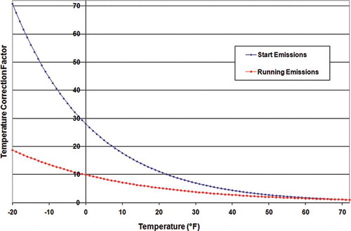
One of the most significant changes in MOVES2010 is temperature adjustments for light-duty vehicle PM exhaust emission rates. The following MOVES2010 PM temperature correction factor (TCF) curves, shown in Figure 1 were applied to the emission factors of GASPM, and OC/EC only (not sulfate) for gasoline and diesel light-duty cars and trucks:

Figure 1. MOVES2010 temperature correction factors for light-duty vehicle PM emission rates, with a basis temperature of 72 ˚F.

(1)

These temperature corrections were applied to temperatures between −20 and 72 ˚F. As in MOVES2010, temperatures 72 ˚F and above were not adjusted.

In even sharper contrast between the two models, MOBILE6 and MOVES2010 estimate evaporative emission processes completely differently. MOVES2010 defines different evaporative processes by means of how emissions are released (e.g., permeation through hoses in the fuel system, liquid leaks, and vapor venting from the fuel tank). MOVES evaporative emissions processes occur both on-road (estimated with gram-per-mile emission rates) and also off-network when the vehicle is parked (gram-per-vehicle emission rates). MOBILE6 separated evaporative emissions modes by vehicle operating status (e.g., running loss during driving, and diurnal for parked vehicles). The evaporative modes between MOVES2010 and MOBILE are not easily cross-referenced, so no MOBILE6 evaporative adjustments were performed as part of this work.

Transportation modeling and traffic counter data

Transportation demand models (TDMs) are primarily used to plan for the expected demand on transportation facilities, but they also can provide a high level of detailed data that greatly improves the accuracy of on-road emission estimates. TDM provides for each link the spatially defined start and end node coordinates, loaded volumes by time period, and a number of other link properties including distance, number of lanes, capacity, free flow speed, and congested speed. TDMs use internal speed adjustments to account for congestion based on period level volumes on links. For TDM outputs describing an average weekday, the time periods are usually multihour groups that correspond to morning and afternoon peak commute hours, a midday period, and an overnight off-peak period. These models are trip based in the sense that vehicle trips have origins and destinations by TAZs that provide the demand basis in order to load the link network by time period. TDMs are often validated with data collected from on-road vehicle counters to refine the model estimates, and that validation data can include counts collected as part of the Federal Highway Administration (FHWA) highway performance monitoring system (HPMS) (Federal Highways Administration). TDM link networks for most urban areas cover all major roads (interstates, freeways, major arterials) and most lesser roads (minor arterials and collectors). The smallest roads—local roads—are not always covered in transportation models, as they are not critical to transportation planning activities. From an emissions standpoint, all activity needs to be accounted for and so CONCEPT can accept non-link-based sources of VMT for local roads provided as a county total. Nonlink VMT are spatially allocated to grid cells by CONCEPT using a spatial surrogate, such as human population.

In addition to TDM traffic volumes by time period, automatic traffic recorder (ATR) continuous traffic count data are used to develop temporal allocation profiles that are used in CONCEPT MV. ATR data are typically available from state and county highway departments, and also may be available from local urban transportation planners, and the data are used to develop total volume temporal profiles for use in CONCEPT MV to allocate multihour traffic volume into individual hours. The total volume profiles are the hourly fraction of the total vehicle volume by roadway type, month, and day of week. In each of the profiles, 24 hourly fractions sum to 1, where each fraction corresponds to the fraction of the total volume occurring during that hour. To avoid biased results, the total volume profiles are developed using only monitor days with 24 hours of complete data. Specialized ATRs at some monitoring sites can distinguish vehicle class based on the number of axles and spacing. Methods developed by Lindhjem and Shepard (2007) were used with vehicle classification counter data to estimate vehicle mix fractions that vary by road type and hour of day, day of week, and month of year to be used in CONCEPT MV for allocating hourly traffic volumes to vehicle classes.

The Southeast Michigan Council of Governments (SEMCOG) (2009) provided the Detroit area TDM vehicle activity data, including speed adjustments, age distributions, and other emission modeling input data. Vehicle classification data used to determine the temporal and road type

VMT mix estimates were also provided by SEMCOG. Figure 2 shows the SEMCOG Detroit area road network. Transportation modelers from the Atlanta Regional Commission (2009) provided the Atlanta area vehicle activity data from their TDM, vehicle fleet, and other emission modeling input parameters, and vehicle classification data used to generate the VMT mix profiles. Figure 3 shows the Atlanta area road link network. Figure 4 shows trip starts and ends by TAZ in the Atlanta metropolitan area where the colors represent the density of trip starts (left) and ends (right) for the morning peak period.

Figure 2. Detroit area road link network.

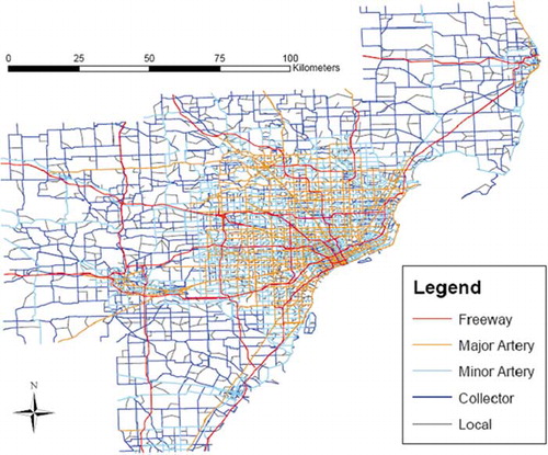
Figure 3. Atlanta area road link network.

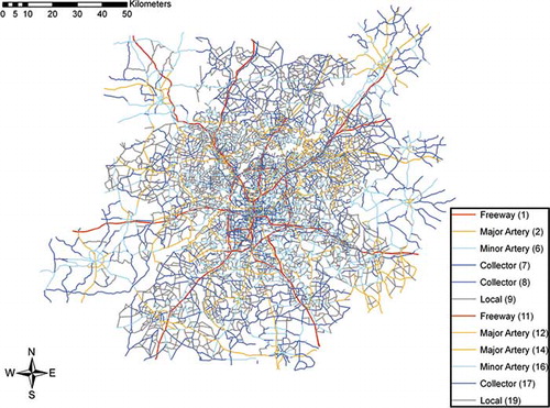
Figure 4. Density of trip starts (left) and ends (right) (trips per acre) for Atlanta on a weekday morning.

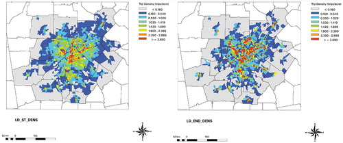
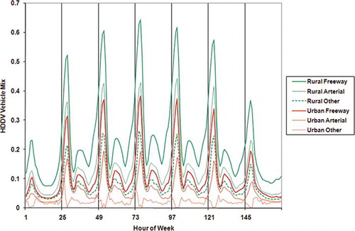
Figure 5. National average HDDV fraction by road type and hour of week (Lindhjem and Shepard, 2007).

CONCEPT MV emission model

The CONCEPT MV on-road vehicle emission model was used to combine link-level vehicle activity with emission factors developed for the vehicle speed and ambient conditions for each link by hour of day, day of week, month of year, and road type. The CONCEPT MV model generates gridded hourly emission estimates ready for input to air quality models such as the Community Multiscale Air Quality (CMAQ) model and the Comprehensive Air quality Model with extensions (CAMx). To incorporate MOVES2010 emission estimates into CONCEPT MV, MOVES2010 was run externally to CONCEPT MV, and CONCEPT MV was altered to read new input files of emission rates (by vehicle class, speed, temperature, and humidity) from MOVES2010 for running exhaust and start emissions. The main steps in the CONCEPT MV model for estimating emissions are as follows.

Temporal allocation of traffic activity

TDMs typically estimate traffic activity in multihour periods, such as morning and afternoon commutes, midday hours, and overnight hours. CONCEPT MV calculates activity for every hour within a TDM time period using total volume temporal profiles developed from analysis of local ATR data to disaggregate the period (multihour) total volumes. The hourly total volume profiles vary by roadway type, day of week, month, and year.

Speed adjustment for congestion

CONCEPT MV reads link free flow speeds and speed adjustment instructions for reducing free flow speed when volumes are high relative to a link's capacity. The speed adjustment instructions can be supplied as a lookup table of adjustments to free flow speed or directly for the commonly used algorithm called the Bureau of Public Roads (BPR) adjustment curve that describes the relationship of speed based on vehicle volumes relative capacity along each link. The lookup table of adjustments can vary by speed as well as volume-capacity ratio, providing a great deal of flexibility in how congested speeds are calculated. Alternatively, users may provide link-level hourly congested speed values directly to CONCEPT MV with no speed adjustment instructions, if the speed data are available.

Spatial allocation

Many emission factors depend on temperature and relative humidity. The vehicle activity data are spatially associated with grid cells so that the grid-cell specific meteorology can be used to determine which emission factor to apply. The link-based VMT data are spatially allocated using an overlay of the link network on the modeling grid. Vehicle populations, county-based VMT data, and TAZ/county-based trip data are allocated to the model grid using spatial surrogates. Link-based VMT data are spatially allocated using an overlay of the link network on the model grid. County-based VMT (such as VMT on local roads) and TAZ trips data are used allocated to the model grid using spatial surrogates.

Application of VMT mix profiles

Total volume on each link is split into vehicle classes using vehicle mix temporal profiles provided as input to CONCEPT MV. The vehicle mix profiles vary by roadway type, time of day, day of week, and month. The vehicle mix profiles are determined from analyses of traffic counter data available from specialized ATRs at some monitoring sites that make continuous counts of vehicles classified by type. These are used to disaggregate total link volumes into by vehicle class volumes by hour and roadway type.

Emission estimation

CONCEPT MV uses the grid cell, county, road type, and link speed to determine the correct emission factor for each vehicle class, pollutant, and gram-per-mile–based emission process for every hour of each episode day. Emissions for each vehicle class, emission type, and pollutant are estimated as the product of the emission factor and the VMT on that link associated with the vehicle class. This applies to running exhaust, running losses, crankcase losses, resting losses, particulate emissions from brake and tire wear, and diurnal emissions. For this work MOVES2010 adjustments to MOBILE6 emission factors were implemented.

For start emissions and hot soak emissions, emission factors in MOBILE6 are provided as either grams per mile or grams per hour per trip. Although the TDMs provide data on the number of trips for each TAZ, and MOBILE6 can provide gram-per-trip emission rates, the TDM trips data are used only in a relative sense to spatially allocate the emissions because the definition of a trip as used in transportation modeling is different from what was used to develop EPA's MOBILE6 trip-based emission rates. Therefore, the data on trips by TAZ are used on a relative basis as follows: CONCEPT MV estimates start and hot soak emissions by multiplying the gram-per-mile emission rates by the VMT for each vehicle type, link, and grid cell. The emissions are summed across the modeling domain and then spatially allocated to the grid cells using the spatial distributions of trips by TAZ. For this work, the MOVES start emissions were estimated as a fraction of the total exhaust in MOVES2010 as described above.

Emission speciation

Emission estimates of criteria pollutants must be speciated for a particular chemical mechanism employed in the air quality model. Chemical speciation profiles are used to allocate VOC and PM emissions to model species. CONCEPT MV applies chemical speciation profiles by vehicle and fuel type, and by emissions source to generate the air quality model-ready speciated emissions. In this work the updated carbon bond mechanism CB05 (Yarwood et al., 2005) was used.

CONCEPT MV modeling scenarios

Regional emission inventories for the Detroit and Atlanta metropolitan areas were prepared using MOBILE6 and MOVES2010 running and start exhaust emissions. The following three modeling scenarios were run for typical summer (July) and winter (January) multiday episodes in 2005 for each city:

1.	Link-level CONCEPT MV with MOBILE6 emission factors, with temporally varying (by hour of day, day of week, and month of year) VMT mix profiles by roadway type. This was the base case scenario.
2.	Link-level CONCEPT MV with MOBILE6 emission factors, with VMT mix profiles that vary by road type, but are flat across all hours and days (no temporal variation). This scenario represents how VMT is typically treated in on-road emission inventories used in air quality modeling.
3.	Link-level CONCEPT MV with MOVES2010 exhaust emissions, with VMT mix fractions varying by roadway type and time.

Comparison of the first and second scenarios provides an investigation of the importance of temporally varying vehicle type fractions, especially with regard to the relative magnitude of heavy-duty diesel and light-duty gasoline vehicle traffic. Comparison of the first and third scenarios shows the impact of the MOVES2010 exhaust emission rates, which are affected by speed and revised temperature adjustments, especially for PM during winter conditions.

Results

The comparisons made for this study were primarily to investigate the importance of temporally varying vehicle mix at link-level spatial scales, and secondarily the use of MOVES2010 emission model on exhaust emissions. Emissions were estimated for the three scenarios described above for metropolitan Detroit and Atlanta, for both winter (January) and summer (July) ambient conditions. For Detroit, the SEMCOG regional analysis considers all weekdays to have equivalent VMT mix, and so episode days Friday through Sunday were modeled. For Atlanta, analysis showed that VMT mix on Fridays differs from the rest of the weekdays, and so episode days Thursday through Sunday were modeled.

Vehicle mix effects

The vehicle mix effect was investigated by comparing estimated emissions derived using one flat weekly average profile per road type (i.e., averaged over all hours and days of a week), as is typically done in modeling, with the base case using vehicle mix profiles that vary by road type, hour of day, and day of week. MOBILE6 emission factors were used for this comparison. Although there are many vehicle classes in both MOBILE6 and MOVES2010, the largest change in emissions is affected by changes in the fraction of heavy-duty diesel vehicle VMT. The HDDV emission effect is seen most significantly with regard to NO_x and PM emissions because the HDDV emission rates for those pollutants are more than an order of magnitude higher than from light-duty vehicles.

Figure 5 shows the national average variation in the fraction of HDDV VMT by roadway type. For all roadway types, the HDDV VMT fraction is significantly lower on weekends than weekdays, more so on Sunday than Saturday. The figure shows the importance of characterizing VMT mix profiles by roadway type, as the HDDV fraction is higher on rural as compared to urban roadways, and significantly higher on freeways as compared to arterials and lesser roads. Also important to note is that the HDDV fraction is reduced significantly in the morning and afternoon commute hours. This same pattern is observed in both the Detroit and Atlanta regions.

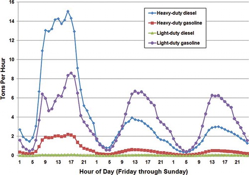
Figure 6 shows Detroit area NO_x emissions by hour and vehicle grouping for each of the three July episode days. For light-duty vehicles, NO_x emissions peak on weekdays during morning and afternoon peak hours, and are higher on weekdays than weekend days. But for heavy-duty diesel vehicles, the weekend NO_x emissions are dramatically lower on weekends because of reduced activity. More importantly, the fraction of VMT from HDDV is small but the fraction of NO_x emissions is very large. During midday hours on weekdays, HDDVs in the Detroit area account for about 8–10% of VMT on interstates, 6–8% of VMT on major arterials, and about 2% on minor arterials, but they account for more than 60% of the NO_x (and PM) emissions during those hours. During predawn hours, HDDVs account for a much higher fraction of emissions (up to about 25% at 5 a.m.) and about 70% of NO_x (and PM) emissions. Apart from the fraction of VMT, other factors that account for changes in HDDV NO_x emissions over the hours of the day include temperature, humidity, and speed.

Figure 6. Detroit area July NO_x emissions by vehicle and fuel type.

Tables 2–5 show the percent change in emissions from using a using a temporally varying profile (base case) to using a flat vehicle mix profile, the latter being what is typically done in current modeling practice. In both Detroit and Atlanta, the largest change in vehicle mix occurs when HDDV traffic decreases from weekdays to weekends. Using a flat vehicle mix profile thus improperly estimates too much HDDV traffic on weekends and overpredicts NO_x and PM emissions on weekends. Conversely, the flat vehicle mix profiles underestimate HDDV activity and emissions during weekdays. Tables 3 and 5 show that these small changes in the fractions of HDV VMT have very large effects on HDDV emissions, and much smaller effects on light-duty gasoline vehicle emissions. These impacts are more significant in Detroit because the HDDV fraction was higher during the weekdays and lower on weekends compared with Atlanta area activity.

Table 3. Percent change in Detroit area NO_x emissions from using temporally varying VMT mix profiles (base case) to using flat vehicle mix profiles

	January Friday		January Sunday		July Friday		July Sunday
Vehicle Type	Base Case(tpd)	Effect(%)	Base Case(tpd)	Effect(%)	Base Case(tpd)	Effect(%)	Base Case(tpd)	Effect(%)
Heavy-duty diesel	181.1	−20.8	36.1	180.2	201.3	−21.9	40.2	174.4
Heavy-duty gas	28.5	−15.8	6.6	159.0	28.9	−17.1	6.6	154.6
Light-duty diesel	1.1	−4.4	0.6	15.6	1.2	−6.0	0.7	12.8
Light-duty gas	157.3	3.9	115.6	−4.8	103.9	2.6	76.7	−6.6
Total	367.9	−9.8	159.0	44	335.3	−13.9	124.3	60.7

Table 4. Percent change in Atlanta area emissions from using temporally varying VMT mix profiles (base case) to using flat vehicle mix profiles

	January		July
Pollutant	Friday	Sunday	Friday	Sunday
TOG	1.8	0.2	0.4	−1.1
NOx	−9.6	5.8	−3.7	16.0
PM10	−5.8	13.5	1.3	20.5
PM2.5	−7.7	19.2	1.7	30.0
CO	1.4	−1.1	0.7	−1.2

Table 5. Percent change in Atlanta area NO_x emissions from using temporally varying VMT mix profiles (base case) to using flat vehicle mix profiles

	January Friday		January Sunday		July Friday		July Sunday
Vehicle Type	Base Case(tpd)	Effect(%)	Base Case(tpd)	Effect(%)	Base Case(tpd)	Effect(%)	Base Case(tpd)	Effect(%)
Heavy-duty diesel	161.5	−22.9	68.3	16.7	138.1	−7.9	59.9	46.2
Heavy-duty gas	9.9	−11.4	5.0	10.7	8.8	−0.7	5.0	20.1
Light-duty diesel	0.6	0.4	0.4	−1.6	0.7	0.2	0.5	−1.5
Light-duty gas	189.2	1.9	116.2	−0.8	149.7	0.0	98.9	−2.4
Total	361.1	−9.6	189.9	5.8	297.3	−3.7	164.3	16.0

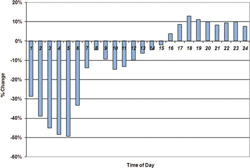
Figure 7 shows the importance of the diurnal variation in vehicle type mix by hour of day. Whereas the change in NO_x emissions for Atlanta on a Friday in July using a flat vehicle mix profile results in a small underprediction (3.7%) of total daily emissions, the morning NO_x emissions are much more significantly underpredicted, by as much as 50% for some hours. This underprediction of morning NO_x emissions would result in an overprediction of morning VOC/NO_x ratios and could thus affect the predictions of afternoon ozone air quality.

Figure 7. Effect of using a flat vehicle mix profile compared to temporally varying vehicle mix profiles on Atlanta NO_x emissions, by hour of day for a July Friday in 2005.

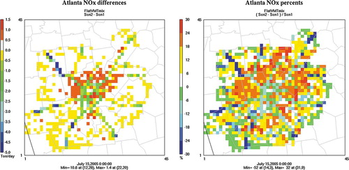
Figure 8 and 9 demonstrate the impact that using one average flat vehicle profile has on the spatial distribution, and on individual grid cells, on PM emissions on a 2005 January Friday in Detroit and NO_x emissions on a 2005 July in Atlanta, respectively. The flat vehicle mix profile underpredicts NO_x and PM emissions on weekdays, with the largest underpredictions on freeways, by 10–30%, where the majority of the HDDV VMT occurs. The more significant underprediction is on rural freeways where the HDDV VMT fraction is largest. The flat vehicle mix profile is more likely to overpredict NO_x and PM on surface roads and usually away from the urban core where there is typically less HDDV traffic. These figures demonstrate that the use of temporally varying VMT mix profiles by roadway type better describes local vehicle emissions.

Figure 8. Effect of using a flat vehicle mix profile on PM emissions for 2005 January Friday in Detroit (left, tons per day difference; right, percentage change from temporally varying vehicle mix).

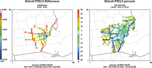
Figure 9. Effect of using a flat vehicle mix profile on NO_x emissions for a 2005 July Friday in Atlanta (left, tons per day difference; right, percentage change from temporally varying vehicle mix).

MOVES2010 versus MOBILE6 emission factor effects

For both the Detroit and Atlanta metropolitan regions, winter (January) and summertime (July) conditions were run to demonstrate the importance of temperature and speed adjustments on emission rates of multiple pollutants. The January episode days ranged from 14 to 22 ˚F in Detroit and 39 to 55 ˚F in Atlanta, whereas the July episode days ranged from 67 to 85 ˚F in Detroit and 74 to 91 ˚F in Atlanta. Weekdays have higher VMT, and in particular higher HDDV VMT. Weekdays typically have lower vehicle speeds, especially during commute hours due to traffic congestion, and the importance of the MOVES2010 speed adjustments on emissions can be observed in the modeling runs performed.

Tables 6 and 8 show the overall effect on vehicle emissions with the use of MOVES2010 exhaust emission rates. In these daily total emissions comparisons, emissions for all pollutants are increased on both weekdays and weekends in both seasons. The MOVES2010 model increases PM_2.5 emission rates in Detroit, and NO_x emissions in Atlanta, for both seasons for virtually all vehicle types except heavy-duty gasoline vehicles (Tables 7 and 9). The influence of temperature corrections on PM_2.5 exhaust emissions is particularly apparent in the January results in Table 7. The low-temperature effect on the gasoline light-duty cars and trucks is notable in that gasoline PM_2.5 emissions become higher than diesel PM_2.5 at low temperatures.

Table 6. Percent change in 2005 Detroit area emissions from MOBILE6 to MOVES2010 exhaust emission rates

	January		July
Pollutant	Friday	Sunday	Friday	Sunday
TOG	36.6	59.7	36.8	47.2
NOx	52.1	64.3	76.1	116.3
PM10	169.6	239.8	60.9	56.8
PM2.5	233.1	383.8	88.5	95.4

Table 7. Change in 2005 Detroit area PM_2.5 emissions from MOBILE6 to MOVES2010 exhaust emission rates, by vehicle type

	January Friday		January Sunday		July Friday		July Sunday
Vehicle Type	Base Case(tpd)	Effect(%)	Base Case(tpd)	Effect(%)	Base Case(tpd)	Effect(%)	Base Case(tpd)	Effect(%)
Heavy-duty diesel	3.5	116.5	0.7	181.4	3.9	120.6	0.8	186.6
Heavy-duty gas	0.4	−62.1	0.1	−60.5	0.4	−61.8	0.1	−60.2
Light-duty diesel	0.1	1156.7	0.1	1221.8	0.1	90.7	0.6	111.9
Light-duty gas	1.5	502.7	1.2	500.5	1.7	50.5	1.3	51.2
Total	5.5	233.1	2.0	383.8	6.19	88.5	2.3	95.4

Table 8. Percent change in 2005 Atlanta area emissions from MOBILE6 to MOVES2010 exhaust emission rates

	January		July
Pollutant	Friday	Sunday	Friday	Sunday
TOG	8.3	15.5	17.4	20.8
NOx	54.9	57.4	61.6	63.8
PM10	108.2	103.1	68.4	57.6
PM2.5	155.6	157.3	103.2	92.4

Table 9. Change in 2005 Atlanta area NO_x emissions from MOBILE6 to MOVES2010 exhaust emission rates, by vehicle type

	January Friday		January Sunday		July Friday		July Sunday
Vehicle Type	Base Case(tpd)	Effect(%)	Base Case(tpd)	Effect(%)	Base Case(tpd)	Effect(%)	Base Case(tpd)	Effect(%)
Heavy-duty diesel	161.5	58.4	68.3	55.6	138.1	58.6	59.9	56.7
Heavy-duty gas	9.9	−38.3	5.0	−39.3	8.8	−49.1	5.0	−50.4
Light-duty diesel	0.6	161.1	0.4	143.1	0.7	155.4	0.5	131.3
Light-duty gas	189.2	56.3	116.2	62.3	149.7	70.5	98.9	73.5
Total	361.1	54.9	189.9	57.4	297.3	61.6	164.3	63.8

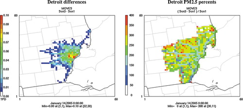
Figure 10 demonstrates the effect of the change from MOBILE6 to MOVES2010 on the predicted PM_2.5 emissions in Detroit in January 2005. The largest emission increases are in the urban core, where vehicle density is highest. Light-duty gasoline vehicle emissions are very sensitive to low ambient temperatures (Figure 1), and consequently PM_2.5 emission increases are larger on surface roads, where fewer HDDV operate. On freeways, HDDV are a more significant fraction of the total emissions (Figure 5), so the percentage increase in PM_2.5 is lower than on surface streets for winter conditions.

In the MOVES2010 scenario, PM emissions from starts were treated as separate emission estimates from running emissions, and CONCEPT MV allocates start emissions to TAZs, not to the road links. In addition, as shown in (Figure 1), the MOVES2010 light-duty cold-temperature adjustment is significantly higher for PM emissions from starts compared to those for running. The right side of Figure 10 shows that the largest percentage increases between the MOBILE6 and MOVES scenarios are in grid cells off the major roads and in the outlying areas of the region, likely demonstrating the importance of cold start PM emission rates.

Figure 10. Effect of using MOVES2010 exhaust emission rates on PM emissions for a Friday in January 2005 for Detroit (left, tons per day difference; right, % change from MOBILE6).

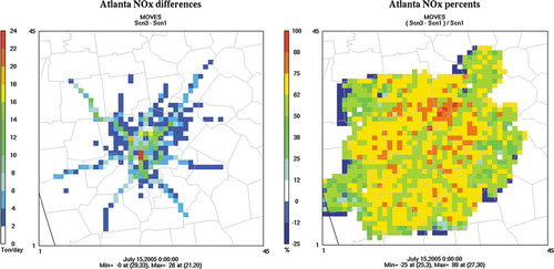
Atlanta NO_x emissions increase for both light- and heavy-duty vehicles (Table 9), and the right side of Figure 11 shows that the percentage increase is widespread and generally uniform over the region in for a July Friday. Figure 11 (left side) shows that the greatest ton-per-day increases are mostly along freeways and in the urban core, where VMT density is high. Nonfreeway links have higher emissions with MOVES2010 because that model estimates higher emissions at lower speeds that are more likely to be observed on smaller roads affected by stop and go conditions, especially during congested commute hours.

Figure 11. Effect of using MOVES2010 exhaust emission rates on NO_x emissions for a Friday in July 2005 for Atlanta (left, tons per day difference; right, % change from MOBILE6).

The use of MOVES2010 for air quality modeling may have a significant effect on ozone and PM_2.5 predictions, especially for historic calendar year episodes. For summertime ozone episodes, MOVES2010 increases NO_x emissions significantly and to a greater extent than exhaust TOG emissions. This will have the effect of increasing predicted NO_x emissions urban area-wide, and especially for local urban core areas where vehicle traffic is highest. CONCEPT MV allows for detailed disaggregation of link-level emission predictions, and the emission effects of using MOVES2010 varies by road type and congestion level. The impact of MOVES2010 on PM_2.5 predictions could be much more significant than for ozone precursors. In addition to the higher overall emission rates, average speed and ambient temperature can substantially increase PM emissions. MOVES2010 will have the greatest impact on wintertime PM predictions for those cities with more extreme winter temperatures. The localized and temporal emission inventory adjustments described in this work can be used to better characterize the ambient PM_2.5 levels. MOVES2010 could have the greatest impact on local-scale emissions. The effect of vehicle speed was previously underappreciated, and MOVES2010 HDDV PM emission rates are considerably higher (by an order of magnitude) at slow speeds.

Conclusions and Future Work

Air quality managers rely on emission models and air quality models to predict future air quality and to evaluate the effectiveness of candidate control measures. It is essential in this regard to characterize vehicle activity and emissions as accurately as possible. With a better understanding of the factors that are important in vehicle emissions, and more sophisticated models, it is possible now to characterize and estimate vehicle emissions in a much more detailed and accurate way than has been previously done. Many studies of weekday/weekend ozone have indicated the importance of better characterizing vehicle activity differences between weekdays and weekends. Understanding and more accurately characterizing changes in hour-to-hour vehicle activity and emissions is also important for ozone modeling, as the morning emissions mix (and in particular the VOC/NO_x ratio) is one of the key determinants of afternoon ozone peaks.

We have demonstrated here that it is critical to accurately characterize the proportion of overall activity (VMT) from heavy-duty diesel vehicles, as the gram-per-mile emission factors for these vehicles can be more than an order of magnitude higher than for light-duty gasoline vehicles. Historically, the typical approach has been to estimate VMT mix and apply that mix uniformly across all roadway types and hours of the day. In recent years, modelers have developed and applied VMT mix profiles by roadway type, which is an important improvement, because HDDVs account for a greater fraction of VMT on freeways than on surface streets. A more significant improvement to vehicle emission estimation is to use available traffic counter and vehicle classification monitoring data to derive temporally varying (by hour of day, day of week, and month) VMT mix profiles that capture important changes in the HDDV fraction over the course of the day. For NO_x and PM in particular, very small changes in the percent of HDDV VMT can result in very large changes in estimated fleet emissions.

With the new MOVES2010 model, emissions are more sensitive to ambient temperature and vehicle speeds. Light-duty PM emissions in particular are highly sensitive to temperature, with exponential increases at very low temperatures. Emissions are also very sensitive to speed, and in MOVES2010 this is especially true for HDDV PM emissions at lower speeds that occur during commute hours on congested roads. Historically, emissions have been estimated using average speeds by roadway type. A more appropriate approach, as presented here, is to estimate emissions on each link for each hour of the day, and to accurately characterize the changes in speed on each link over the course of the day.

In the Detroit and Atlanta areas and pollutants modeled, emissions increased significantly with the use of MOVES2010 exhaust emission factors as compared to the previous MOBILE6 regulatory model. Emission increases are substantial for NO_x and PM emissions across all road types. Because of the increased sensitivities in MOVES2010 to speeds, temperatures, and VMT mix, it is becoming increasingly important to characterize vehicle activity and ambient conditions in a more detailed manner than has been done previously. The CONCEPT MV model described here can be used to apply temporally varying VMT mix profiles, link-specific VMT and speeds, adjusted speeds for congestion, and gridded temperatures to more accurately estimate vehicle emissions. Since the work reported here was completed, the CONCEPT MV model has been revised to fully incorporate MOVES2010a emission rates for all emission processes (gram/mile and gram/vehicle) directly using the MOVES lookup table output formats. The CONCEPT MV code was substantially revised and new functionality was added to address the new vehicle population-based emission rates that MOVES uses. Improved on-road vehicle emission inventory estimation involves not only estimating appropriate regional scale totals but also including more detailed spatial and temporal allocation factors coupled with the vehicle activity and episodic climate conditions, which CONCEPT MV uses.

Work now in progress uses MOVES2010a emission factors in CONCEPT MV to generate link-based hourly gridded mobile source emission inventories for air quality modeling. The next step is to perform the air quality modeling with these highly temporally and spatially resolved emission inventories, and to compare the air quality modeling predictions with air quality modeling using mobile source emissions that have not been that highly resolved.

Acknowledgments

The authors wish to acknowledge the members of the MOVES team of the EPA Office of Transportation and Air Quality for helpful suggestions on incorporating MOVES emission estimates with vehicle activity data, and the Atlanta Regional Commission (ARC) and Southeast Michigan Council of Government (SEMCOG) for the travel network input data and helpful suggestions on how to use the data. This work was funded by the Electric Power Research Institute.

References

- Geophysics , Alpine . June 2006 2006 . Development of Version Two of the California Integrated Transportation Network (ITN) , June 2006 , Sacramento , CA : Technical Report AG-TS-90/210. Prepared for CalEPA-Air Resources Board, Planning and Technical Support Division .
- Atlanta Regional Commission . 2009 . “ Personal Communication with Guy Rousseau, Jonathan Morton, Georgia Department of Natural Resources Environmental Protection, and Robert W. Goodwin, Georgia Regional Transportation Authority ” .
- Bai , S. , Chiu , Y.-C. and Niemeier , D.A. 2007 . A comparative analysis of using trip-based versus link-based traffic data for regional mobile source emissions estimation . Atmos. Environ , 41 : 7512 – 7523 .
- Bai , S. , Nie , Y. and Niemeier , D. 2007 . The impact of speed post-processing methods on regional mobile emissions estimation . Transport. Res. Part D Transport Environ. , 12 : 307 – 324 .
- Blanchard , C.L. and Tanenbaum , S.J. 2003 . Differences between weekday and weekend air pollutant levels in southern California . J. Air Waste Manage. Assoc. , 53 : 816 – 828 .
- Blanchard , C.L. and Tanenbaum , S.J. 2006 . Weekday/weekend differences in ambient air pollutant concentrations in Atlanta and the southeastern U.S . J. Air Waste Manage. Assoc. , 56 : 271 – 284 .
- Blanchard , C.L. , Tanenbaum , S.J. and Lawson , D.R. 2008 . Differences between weekday and weekend air pollutant levels in Atlanta; Baltimore; Chicago; Dallas-Fort Worth; Denver; Houston; New York; Phoenix; Washington, DC; and surrounding areas . J. Air Waste Manage. Assoc. , 58 : 1598 – 1615 . doi: 10.3155/1047–3289.58.12.1598
- Chinkin , L.R. , Coe , D.L. , Funk , T.H. , Hafner , H.R. , Roberts , P.T. and Ryan , P.A. 2003 . Weekday versus weekend activity patterns for ozone precursor emissions in California's South Coast Air Basin . J. Air Waste Manage. Assoc. , 53 : 829 – 843 .
- Cook , R. , Brzezinski , D. , Michaels , H. , Touma , J.S. , Beidler , A. and Strum , M. May 15–18 2006 . “ Use of travel demand model data to improve inventories in Philadelphia. Presented at the 15th International Emission Inventory Conference of the U.S. Environmental Protection Agency ” . May 15–18 , New Orleans , LA 2006
- Cook , R. , Isakov , V. , Touma , J.S. , Benjey , W. , Thurman , J. , Kinnee , E. and Ensley , D. 2008 . Resolving local-scale emissions for modeling air quality near roadways . J. Air Waste Manage. Assoc. , 58 : 451 – 461 . doi: 10.3155/1047–3289.58.3.451
- Dallmann , T.R. and Harley , R.A. 2010 . Evaluation of mobile source emission trends in the U.S . J. Geophys. Res. , 115 : D14305
- Elkus , B. and Wilson , K.R. 1976 . Photochemical air pollution: Weekend–weekday differences . Atmos. Environ. , 11 : 509 – 515 .
- Federal Highways Administration. 2012. Highway Performance Monitoring System (HPMS) http://www.fhwa.dot.gov/policy/ohpi/hpms/index.cfm (http://www.fhwa.dot.gov/policy/ohpi/hpms/index.cfm)
- Fujita , E.M. , Stockwell , W.R. , Campbell , D.E. , Keislar , R.E. and Lawson , D.R. 2003 . Evolution of the magnitude and spatial extent of the weekend ozone effect in California's South Coast Air Basin, 1981 to 2000 . J. Air Waste Manage. Assoc. , 53 : 802 – 815 .
- Graedel , T.E. , Farrow , L.A. and Weber , T.A. 1977 . Photochemistry of the Sunday effect . Environ. Sci. Technol. , 11 : 690 – 694 .
- Harley , R. , Marr , L. , Lehner , J. and Giddings , S. 2005 . Changes in motor vehicle emissions on diurnal to decadal time scales and effects on atmospheric composition . Environ. Sci. Technol. , 39 : 5356 – 5362 .
- Heuss , J.M. , Kahlbaum , D.F. and Wolff , G.T. 2003 . Weekday/weekend ozone differences: What can we learn from them? . J. Air Waste Manage. Assoc. , 53 : 772 – 788 .
- Jung , L. January 31, 2011 2011a . Maricopa Association of Governments , January 31, 2011 , Phoenix , AZ : MOVESLink Technical Memo to Taejoo Shin .
- Jung , L. May 6, 2011 2011b . Maricopa Association of Governments May 6, 2011 , Phoenix , AZ. MOVESLink Technical Memo to Allison DenBleyker
- Koo , B. , Jung , J. , Pollack , A.K. , Lindhjem , C. , Jimenez , M. and Yarwood , G. 2011 . Impact of meteorology and anthropogenic emissions on the local and regional ozone weekend effect: the case of Midwestern US . review ,
- Lawson , D.R. 2003 . Forum—The weekend ozone effect—The weekly ambient emissions control experiment . Environ. Manager , July : 17 – 25 .
- Levitt , S. and Chock , D. 1976 . Weekday–Weekend pollutant studies of the Los Angeles Basin . J. Air Pollut. Control Assoc. , 26 : 1091 – 1092 .
- Lindhjem, C.E., and S. Shepard. 2007. Development Work for Improved Heavy-Duty Vehicle Modeling Capability Data Mining–FHWA Datasets. EPA-600/R-07/096. Washington, DC: U.S. Environmental Protection Agency, U.S. Government Printing Office http://www.epa.gov/nrmrl/pubs/600R07096/600r07096.htm (http://www.epa.gov/nrmrl/pubs/600R07096/600r07096.htm) (Accessed: 29 February 2012 ).
- Marr , L.C. and Harley , R.A. 2002 . Modeling the effect of weekday-weekend differences in motor vehicle emissions on photochemical air pollution in central California . Environ. Sci. Technol. , 36 : 4099 – 4106 .
- Pollack, A.K., J. Haasbeek, and M. Janssen. 2005. Development of link-level mobile source emission inventories. Presented at 14th International Emission Inventory Conference of the U.S. Environmental Protection Agency, Las Vegas, NV, April 11–14, 2005 http://www.epa.gov/ ttn/chief/conference/ei14/index.html (http://www.epa.gov/ ttn/chief/conference/ei14/index.html)
- Southeast Michigan Council of Governments (SEMCOG) . 2009 . Personal communication with Joan Weidner
- Texas Transport Institute (TTI) . August 2010 2010 . Production of MOVES On-Road Mobile, Link-Based Emissions Estimates and Document Preparation , August 2010 , Austin , TX : Technical Report, Study No. 403421-0. Prepared for Texas Commission on Environmental Quality .
- Torres-Jardon , R. and Keener , T.C. 2006 . Evaluation of ozone-nitrogen oxides-volatile organic compound sensitivity of Cincinnati, Ohio . J. Air Waste Manage. Assoc. , 56 : 322 – 333 .
- U.S. Environmental Protection Agency (EPA), Office of Air and Radiation. 1997. U.S. Emission standards reference guide for heavy-duty and nonroad engines, September 1997 http://www.epa.gov/oms/cert/hd-cert/stds-eng.pdf (http://www.epa.gov/oms/cert/hd-cert/stds-eng.pdf)
- U.S. Environmental Protection Agency (EPA), Office of Transportation and Air Quality. 2007. Summary of current and historical light-duty vehicle emission standards, April 2007 http://www.epa.gov/greenvehicles/detailedchart.pdf (http://www.epa.gov/greenvehicles/detailedchart.pdf)
- U.S. Environmental Protection Agency (EPA), Office of Transportation and Air Quality. 2008. Analysis of Particulate Matter Emissions from Light-Duty Gasoline Vehicles in Kansas City. EPA-420-R-08/010 , Washington , DC : U.S. Government Printing Office .
- U.S. Environmental Protection Agency (EPA). 2012a. U.S. Environmental Protection Agency Modeling and Inventories http://www.epa.gov/ otaq/models.htm (http://www.epa.gov/ otaq/models.htm)
- U.S. Environmental Protection Agency (EPA). 2012b. U.S. Environmental Protection Agency Modeling and Inventories, MOVES http://www.epa.gov/otaq/models/moves/index.htm (http://www.epa.gov/otaq/models/moves/index.htm)
- U.S. Environmental Protection Agency (EPA). 2012c. U.S. Environmental Protection Agency Technology Transfer Network Clearinghouse for Inventories & Emissions Factors, Emissions Modeling Clearinghouse Temporal Allocation http://www.epa.gov/ttn/chief/emch/temporal/ (http://www.epa.gov/ttn/chief/emch/temporal/)
- U.S. Environmental Protection Agency (EPA). 2012d. U.S. Environmental Protection Agency Technology Transfer Network Clearinghouse for Inventories & Emissions Factors, Emissions Modeling Clearinghouse Related Spatial Allocation Files—“New” Surrogates http://www.epa.gov/ttn/chief/emch/spatial/ newsurrogate.html (http://www.epa.gov/ttn/chief/emch/spatial/ newsurrogate.html)
- Venugopal , M. June 2–5 2008 . “ EmiLink: Mobile source air toxic analysis tool. Presented at 17th International Emission Inventory Conference of the U.S. Environmental Protection Agency ” . June 2–5 , Portland , OR 2008
- West Virginia University . August 2007 2007 . Heavy-Duty Vehicle Chassis Dynamometer Testing for Emissions Inventory, Air Quality Modeling, Source Apportionment and Air Toxics Emissions Inventory , August 2007 , Prepared for Coordinating Research Council, Inc.; California Air Resources Board; U.S. Environmental Protection Agency; U.S. Department of Energy Office of FreedomCAR; Vehicle Technologies through the National Renewable Energy Laboratory, South Coast Air Quality Management District; Engine Manufacturers Association . Report No. CRC E55/57
- Yarwood , G. , Grant , J. , Koo , B. and Dunker , A.M. 2008 . Modeling weekday to weekend changes in emissions and ozone in the Los Angeles Basin for 1997 and 2010 . Atmos. Environ. , 42 : 3765 – 3779 .
- Yarwood, G., S. Rao, M. Yocke, and G.Z. Whitten. December 2005. Updates to the Carbon Bond Mechanism: CB05. U.S. Environmental Protection Agency Report RT–04–00675. Novata, CA: ENVIRON International Corporation http://www.camx.com/publ/ (http://www.camx.com/publ/)
- Yarwood , G. , Stoeckenius , T.E. , Heiken , J.G. and Dunker , A.M. 2003 . Modeling weekday/weekend ozone differences in the Los Angeles region for 1997 . J. Air Waste Manage. Assoc. , 53 : 864 – 875 .