Prediction of daily fine particulate matter concentrations using aerosol optical depth retrievals from the Geostationary Operational Environmental Satellite (GOES)

Abstract

Although ground-level PM_2.5 (particulate matter with aerodynamic diameter <2.5 μm) monitoring sites provide accurate measurements, their spatial coverage within a given region is limited and thus often insufficient for exposure and epidemiological studies. Satellite data expand spatial coverage, enhancing our ability to estimate location- and/or subject-specific exposures to PM_2.5. In this study, the authors apply a mixed-effects model approach to aerosol optical depth (AOD) retrievals from the Geostationary Operational Environmental Satellite (GOES) to predict PM_2.5 concentrations within the New England area of the United States. With this approach, it is possible to control for the inherent day-to-day variability in the AOD-PM_2.5 relationship, which depends on time-varying parameters such as particle optical properties, vertical and diurnal concentration profiles, and ground surface reflectance. The model-predicted PM_2.5 mass concentration are highly correlated with the actual observations, R ² = 0.92. Therefore, adjustment for the daily variability in AOD-PM_2.5 relationship allows obtaining spatially resolved PM_2.5 concentration data that can be of great value to future exposure assessment and epidemiological studies.

Implications:

The authors demonstrated how AOD can be used reliably to predict daily PM_2.5 mass concentrations, providing determination of their spatial and temporal variability. Promising results are found by adjusting for daily variability in the AOD-PM_2.5 relationship, without the need to account for a wide variety of individual additional parameters. This approach is of a great potential to investigate the associations between subject-specific exposures to PM_2.5 and their health effects. Higher 4 × 4-km resolution GOES AOD retrievals comparing with the conventional MODerate resolution Imaging Spectroradiometer (MODIS) 10-km product has the potential to capture PM_2.5 variability within the urban domain.

Introduction

Routine measurements of ground-level PM_2.5 (particulate matter with aerodynamic diameter <2.5 μm) concentrations by air quality monitoring networks are of great importance in assessing exposures, but their spatial coverage is limited and often insufficient for epidemiological studies. Satellite remote sensing adds another important tool to retrieve for aerosol properties, due to global repeated observations of the earth surface and atmosphere, and is often the only source of PM_2.5 data in areas where no ground monitoring stations are available (Wang and Christopher, 2003). The most common parameter derived from satellite observations is the aerosol optical depth (AOD), which is a measure of the extinction of electromagnetic radiation at a given wavelength due to the presence of aerosols in an atmospheric column.

Many studies have examined the relationship between total-column AOD and surface PM_2.5 measurements. Hoff and Christopher (2009) reviewed more than 30 papers that investigated the relationship between total-column AOD and surface PM_2.5 measurements. Most have developed linear regressions between the satellite-measured AOD and the PM_2.5 mass concentrations measured at the ground (Engel-Cox et al., 2004; Wang and Christopher, 2003). More recent investigations have often used ancillary information such as boundary layer height, humidity, and other variables to better relate AOD and PM_2.5 (Gupta et al., 2006; Koelemeijer et al., 2006; Liu et al., 2005). Several studies have employed light detection and ranging (LIDAR) instruments to capture the vertical aerosol distribution at specific locations (Engel-Cox, 2006; Schaap et al., 2009). These studies from across the globe have reported a wide range of correlations between AOD and PM_2.5 mass.

As mentioned above, the relationship between column AOD and PM_2.5 is affected by a variety of parameters. These include relative humidity, mass extinction efficiency, hygroscopic growth factor, vertical distribution of aerosols, aerosol size distribution, and variability in surface reflectance (Wang and Christopher, 2003; Kaufman and Fraser, 1983). Recently, we proposed that the effects of these time-varying parameters influencing the AOD-PM_2.5 relationship can be taken into account with daily adjustments (Lee et al., 2011). This approach was used to accurately predict PM_2.5 concentrations using the MODerate resolution (10 × 10 km) Imaging Spectroradiometer (MODIS) AOD measurements. Regrettably, the MODIS instrument is reaching the end of its design life and will be replaced by Visible Imaging Infrared Radiometer Suite (Report 1, http://www.nasa.gov/mission_pages/NPP/main/).

For the North America region, the National Oceanic and Atmospheric Administration Geostationary Operational Environmental Satellite (NOAA GOES) provides the Aerosol and Smoke Product (GASP) at a higher spatial resolution (4 × 4 km) and temporal resolution (every 30 min) compared with the once-a-day polar-orbiting MODIS sensor. However, the GASP AOD retrievals are less precise than those from the polar-orbiting instruments because of the sensor's coarse spectral resolution and fixed viewing geometry (Prados et al., 2007). Despite these limitations, GASP AOD retrievals were shown to be reasonably well correlated (albeit less precise than MODIS) with Aerosol Robotic Network (AERONET) ground measurements of the total aerosol column for the northeastern United States. (Prados et al., 2007). Will our approach overcome the retrieval limitations?

In this study, we explore whether it is possible to obtain accurate estimates of PM_2.5 concentrations using GASP AOD retrieval with a resolution of 4 × 4 km, on a regional scale (∼100–250 km), conducted for the New England area, in the northeastern part of United States. Our goals are to explore the inherent variability of the AOD-PM_2.5 relationship on a daily basis and to show how this variability can be captured by a mixed-effects model approach during the period of April 24 (starting day of GOES-12 East satellite data) through December 31, 2003. Finally, we present the modeled spatial pattern of PM_2.5 levels within the study domain.

Methods

Ground-level PM_2.5 data

Twenty-four-hour integrated PM_2.5 concentrations measured at 26 U.S. Environmental Protection Agency (EPA) PM_2.5 monitoring sites were used to adjust satellite data (Figure 1). These sampling sites include 15 sites from Massachusetts (MA) and 11 sites from Connecticut (CT), during the period of April 24, 2003, through December 31, 2003. Sampling frequency differed by site and included samples collected every day, every third day, and every sixth day. Because AOD from NOAA/GOES has a high temporal resolution, it is possible to adjust hourly PM_2.5 measurements. For the small number of PM_2.5 sites that provide hourly concentration data, we used daily average PM_2.5 concentrations.

Figure 1. PM_2.5 monitoring site locations within the study domain.

Satellite data

The National Oceanic and Atmospheric Administration/National Environmental Satellite Data and Information Service (NOAA/NESDIS) provides near-real-time aerosol optical depth (AOD) from the Geostationary Operational Environmental Satellite (GOES-12 East) Imager known as the GOES Aerosol and Smoke Product (GASP) (Knapp, 2002; Knapp et al., 2005; Kondragunta et al., 2008). The imager measures the top-of-the-atmosphere radiance in one visible channel and four infrared channels. The AOD retrieval uses only the visible (520–720 nm) channel to assess surface reflectivity and atmospheric and aerosol properties. The cloud mask is determined from the visible channel and the two infrared channels: channel 2 (3900 nm) and 4 (10,700 nm) (Kondragunta et al., 2008; Prados et al., 2007). An additional advantage of GOES is its half-hourly temporal coverage that provides much more opportunity for avoiding clouds at least once each day. Regression of GASP AOD values against AOD ground measurements at 10 northeastern U.S. and Canadian sites during 2003–2007 found correlation coefficients in the range of 0.68–0.79 (Prados et al., 2007).

GOES AOD data for April 24 through December 31, 2003, were obtained from NOAA/NESDIS. Data were screened for outliers based on threshold criteria to avoid cloud contamination, cloud shadows, and bright surfaces (Knapp, 2002; Knapp et al., 2005; Kondragunta et al., 2008; Prados et al., 2007). Specifically, AOD values were discarded when (1) they were greater than 2.0; (2) the surface reflectivity was less than 0.5% or greater than 15%; (3) the standard deviation of the AOD over a 3 × 3-pixel box surrounding each 4 × 4-km pixel was greater than 0.2; and (4) the cloud-screening algorithm identified a cloud for that pixel. In addition, we averaged AOD measurements corresponding to 11:15 a.m. to 5:15 p.m. local time to generate daytime AOD estimates. During this time frame, the root mean square (rms) difference of GASP AOD versus ground AERONET AOD was the lowest, being considerably higher at both the beginning and end of the day (Prados et al., 2007). This is due to cloud shadows, which are more prevalent at high solar zenith angles.

Overall, 165 AOD retrieval days were available during the studied period. Because the median number of AOD retrievals per day was 6, the daily average GASP AOD was expected to create higher temporal coverage compared with the snapshots taken by polar-orbiting satellite sensors such as MODIS. Negative AOD values, caused by errors in surface reflectivity estimation, were included because they provide useful information on low-AOD situations (Paciorek et al., 2008). In addition, we created a 4-km resolution grid for data spatial alignment and full-domain prediction. We selected this spatial resolution to match the nominal resolution of the satellite data. To assign AOD values to the regular 4-km modeling grid, we created a network of Thiessen polygons in ArcGIS (version 9.3; Earth System Research Laboratory [ESRI]), each of which is a rectangle with an area of 16 km². We calculated the AOD value for each 4-km grid cell as the area-weighted average of the AOD values of the Thiessen polygons intersecting with this cell. AOD values at each corresponding EPA site were determined according to the matched grid cell in which the site falls.

AOD-PM_2.5 relationship

We investigated the associations between AOD and PM_2.5 measurements. Toward this end, we used AOD data corresponding to snow-free and clear-sky observations and PM_2.5 daily measurements conducted at the sampling sites. Because these relationships between AOD and PM_2.5 measurements vary daily, mixed-effects models were used to allow for the regression intercepts and slopes to vary daily. This modeling approach is presented in the next section.

Mixed-effects model approach

A mixed-effects model approach is a generalization of the standard linear model that incorporates both fixed and random effects, thus enabling the analyses of data generated from several sources of variation. This model approach accounts for day-to-day variability. A basic assumption is that the relationship varies daily because it depends on time-varying parameters such as relative humidity, PM_2.5 vertical and diurnal concentration profiles, PM_2.5 optical properties, and surface reflectance. In a recent paper, we showed that the mixed-effects model approach provides higher accuracy and precision in predicting PM_2.5 concentrations based on the MODIS AOD data set than a simple regression model (Lee et al., 2011). In the present study, we use this model approach to predict PM_2.5 concentrations based on GOES AOD retrievals. Toward this end, quantitative relationships between PM_2.5 concentrations measured at the 26 PM_2.5 monitoring sites and AOD values in their corresponding grid cells were derived. We used the following mixed-effects model with random intercepts and slopes ( eq 1):

(1)

where PM _ij is the PM_2.5 concentration at a spatial site i on day j; AOD _ij is the AOD value in the grid cell corresponding to site i on day j; α and u _j are the fixed and random intercepts, respectively; β ₁ and v _j are the fixed and random slopes, respectively; S _i ∼ N(0, σ _s ²) is the random intercept of site i; ϵ _ij ∼ N(0, σ²) is the error term at site i on a day j and Σ_β is the variance-covariance matrix for the random effects. The AOD fixed effect in the model ( eq 1) accounts for the effect of AOD on PM_2.5, which was the same for all study days. The AOD random effects explain the daily variability in the AOD-PM_2.5 relationship. It is also critical to add a site term as a random effect. In fact, the AOD value in a 4 × 4-km grid cell is an average optical depth in the given grid cell corresponding to an overall relatively low pollution area, whereas the PM_2.5 measurement can indicate relatively high pollution levels due to site proximity to heavy vehicular traffic areas. The solution of the mixed-effects model equations is a maximum likelihood, a form of estimation that accounts for the parameters in the fixed-effects structure of the model to reduce the bias in the covariance parameter estimates (Lindstrom and Bates, 1988; Laird and Ware, 1982). Currently, this is the method implemented for the SAS statistical software package (proc mixed; SAS Institute, Cary, NC).

Days with less than two matched AOD-PM_2.5 measurements were excluded from the analysis. This resulted in the exclusion of 25 days. Subsequently, the model prediction was examined for each day using the root mean squared error (RMSE) between the measured and predicted PM_2.5 concentrations. Fifteen days with high RMSE values (>5 µg m⁻³) were excluded because the AOD-PM_2.5 relationships were not considered reliable, possibly due to errors in estimation of AOD.

Finally, PM_2.5 concentrations for each grid cell on a day j were estimated using the corresponding AOD values as follows:

(2)

The fixed and random intercepts and the fixed and random slopes for each study day were derived previously from eq 1. Note that the random estimates for the site term were excluded. In this way AOD values were unbiased and representative of their corresponding grid cell.

Importantly, it should be noted that the 6-hr GOES AOD values (11:15 a.m. to 5:15 p.m.) were used to estimate 24-hr average PM_2.5 concentrations. However, if we assume that on a given day the (6-hr PM_2.5)/(24-hr PM_2.5) concentration ratio does not vary considerably across sites, then the 6-hr mean AOD values are adequate to predict the 24-hr concentrations. This is because the daily adjustment takes into account the concentration differences between these two time intervals for each day.

Model validation

We use a cross-validation (CV) approach to evaluate the ability of the model to predict PM_2.5 concentrations for each pixel in the study area. Thus, the data set was repeatedly randomly divided into 90% (calibration) and 10% (held-out test) splits. We applied the fitted calibration model to estimate PM_2.5 for the held-out test set. This “out-of-sample” process was repeated 10 times to calculate the cross-validated (CV) R ² values. Subsequently, the predicted PM_2.5 concentrations were compared with those measured at each site. In addition, we examined the relationship between the average measured and predicted PM_2.5 concentrations for each site using Pearson correlation coefficients. To examine the model accuracy, we estimated the coefficient of determination (R ²) between the measured and predicted PM_2.5 concentrations. Finally, the model precision was estimated as the square root of the mean of the squared errors, and % precision was calculated as follows:

(3)

Estimation of PM_2.5 levels in the study domain and their spatial variability

First, daily PM_2.5 concentrations were estimated for each of the 5570 grid cells. Because the AOD retrieval rate varies by location, the number of PM_2.5 concentration predictions varied by grid cell. Therefore, a direct comparison among cell means would not be suitable for the investigation of the PM_2.5 spatial patterns within the study domain. To minimize the potential impact of varying number of PM_2.5 predicted concentrations per grid cell, we first calculated regional PM_2.5 concentrations by averaging the PM_2.5 concentrations for the corresponding day, measured by the EPA stations. Because the number of AOD retrievals varied by day, the number of available PM_2.5 concentrations used to estimate the daily regional average levels varied by day as well. To obtain reasonably reliable and representative regional PM_2.5 concentrations, we use our daily regional PM_2.5 estimations only for days with 50 or more grid cell predictions. Next, we estimated the mean difference between two parameters: predicted PM_2.5 concentration per grid and regional PM_2.5 concentrations for the days where predictions were available. Finally, the estimated grid cell-specific PM_2.5 mean differences were mapped using ArcGIS. Positive mean differences, expressed in µg m⁻³, indicate that on average levels at a given grid cell are higher relative to the regional average PM_2.5 levels, whereas the opposite is true for negative values.

Results

Descriptive statistics

Table 1 summarizes the mean PM_2.5 concentrations measured at the 26 EPA PM_2.5 monitoring sites during our study period.

As can be seen, the mean PM_2.5 concentrations ranges from 9.4 (CV = 0.65) µg m⁻³ in Haverhill, MA (Site ID: 25-009-5005) to 16.0 (CV = 0.69) µg m⁻³ in New Haven, CT (Site ID: 09-009-0018). Many of the monitoring sites showed similar mean PM_2.5 concentrations. The mean PM_2.5 concentration at the New Haven site was higher compared with those monitored at other sites, presumably due to its proximity to the interstate highway I-95. Furthermore, Table 1 presents the site bias estimates for each of the 26 EPA PM_2.5 monitoring sites and their P value determined using the mixed-effects model ( eq 1). As can be seen, the random-effect estimates of the site term were positive for relatively high traffic and populated areas such as New Haven, West Haven, Danbury, and Stamford. These results suggest that it is important to include site bias in a calibration model.

Table 1. Site bias (μg m^{− 3}) estimates for 26 EPA PM_2.5 monitoring sites

Site ID	City	N	Mean	CV	Bias	P value
09-001-0010	Bridgeport, CT	73	13.1	0.74	0.8	0.2
09-001-0113	Bridgeport, CT	69	12.5	0.70	0.9	0.2
09-001-1123	Danbury, CT	80	13.4	0.52	1.3	0.03
09-001-2124	Stamford, CT	74	14.2	0.66	1.2	0.04
09-001-3005	Norwalk, CT	76	13.3	0.69	1.2	0.05
09-001-9003	Westport, CT	79	12.3	0.64	0.2	0.7
09-003-1003	E. Hartford, CT	234	11.5	0.70	−0.6	0.2
09-003-1018	Hartford, CT	78	12.9	0.66	−0.1	0.8
09-009-0018	New Haven, CT	228	16.0	0.67	4.0	<0.0001
09-009-0026	New Haven, CT	69	12.1	0.70	0.4	0.5
09-009-1123	New Haven, CT	81	14.2	0.70	1.2	0.04
09-009-2008	New Haven, CT	74	12.3	0.80	−0.3	0.6
09-009-2123	Waterbury, CT	80	12.8	0.68	−0.1	0.8
09-009-8003	W. Haven, CT	74	13.0	0.79	1.5	0.01
09-011-3002	Norwich, CT	71	11.7	0.66	−1.0	0.1
25-005-1004	Fall River, MA	71	10.3	0.77	−1.0	0.2
25-009-2006	Lynn, MA	74	10.5	0.64	−2.1	0.001
25-009-5005	Haverhill, MA	68	9.4	0.65	−2.5	<0.0001
25-013-0008	Chicopee, MA	192	10.2	0.98	−2.3	<0.0001
25-013-0016	Springfield, MA	201	12.6	0.75	0.2	0.7
25-013-2009	Springfield, MA	60	11.6	0.70	−0.8	0.2
25-023-0004	Brockton, MA	82	9.7	0.71	−1.3	0.04
25-025-0027	Boston, MA	206	11.8	0.55	0.3	0.5
25-025-0042	Boston, MA	205	11.5	0.62	−1.4	0.007
25-025-0043	Boston, MA	77	13.0	0.59	0.4	0.6
25-027-0020	Worcester, MA	143	10.8	0.63	−1.1	0.004
Notes: CV represents coefficient of variation. Bias represents the random-effect estimates of the site term in the mixed-effects model.

Because the sampling frequency of EPA stations is different and included samples collected every day, every third day, and every sixth day, the number of samples used to estimate mean concentrations also varied by site.

Comparison of GOES-retrieved AOD with EPA-measured PM_2.5 concentrations

As mentioned in Mixed-Effects Model Approach (above), 15 days with high RMSE values (>5 µg m⁻³) were excluded from our model. Two possible sources of high RMSE can be considered. First, there are errors in estimating of AOD during low-pollution days above bright surfaces and during snowfall. For instance, because high RMSE was observed on clear low-pollution days with averaged measured PM_2.5 around 2–4 μg m⁻³, these days were excluded (August 2 and August 13, October 6 and October 13, and November 3 and November 10). This is consistent with the study by Prados et al. (2007) that GOES retrieval is more biased at low AOD ranges. Second, there are some days with negative correlations between PM_2.5 and AOD. Our data set demonstrated that these days were characterized by transparent atmosphere (low AOD) but high measured PM_2.5 concentrations, and/or by dirty atmosphere (high AOD) with low measured ground concentrations. For instance, for June 24 and 27–28, large AOD values were caused mostly by the aerosols aloft.

Indeed, whereas the satellite-derived AOD is a measure of particle column in ambient conditions (e.g., variable humidity and consequently variable amounts of water adsorbed on particles), PM_2.5 mass is a measure of dry particles near the surface; therefore, these two parameters are not expected to be strictly correlated. Figure 2 shows the relationship between GOES AOD values and the corresponding 24-hr integrated PM_2.5 concentrations measured at the 26 EPA sites in New England during the study period, with the coefficient of determination of R ² = 0.24.

Figure 2. The relationship between column aerosol optical depth (AOD) derived from the GOES satellite and 24-hr integrated PM_2.5 concentrations measurements at the 26 EPA sites in New England.

To get additional insight into the relationship between AOD and PM_2.5, in Figure 3 we plot (1) different ranges of AOD conditional on PM_2.5 concentrations; and (2) different ranges of PM_2.5 mass conditional on satellite-derived AOD values.

Figure 3. (a–c) Frequency distributions of AOD values as a function of PM_2.5 concentrations. (d–f) Frequency distribution of PM_2.5 mass as a function of AOD values.

Figure 3a shows that although, in general, low AOD values correspond to low measured PM_2.5 concentrations at the ground, occasionally low AOD values correspond to high measured PM_2.5 concentrations. For example, low AOD values and high measured ground concentrations can be observed during very clear winter days when most of the pollution is near the ground and there is a shallow boundary layer. In other words, near-surface PM_2.5 concentrations do not reflect the total AOD column values. For example, December 27–29 were characterized by such conditions and were excluded from our model (Figure 3a; highlighted by arrow). Although Figure 3c also shows that, in general, high AOD values correspond to high PM_2.5 concentrations, high AOD values were observed for some days with low PM_2.5 concentrations, indicating that pollution at upper levels can be higher than what is observed at the ground. Similar relations between PM_2.5 and AOD are shown in Figure 3d–f. Figure 3d shows that although some low PM_2.5 values correspond to relatively high AOD values, some moderate ground PM_2.5 concentrations correspond to low retrieved AOD values (Figure 3e and f). The results in Figure 3 show that the simple approach that calculates PM_2.5-AOD slopes separately for each day in the study can yield highly variable slope estimates. An alternative approach that pools daily slope estimates but uses data from all days to stabilize the estimates takes into account variable factors influencing AOD-PM_2.5 relationships.

PM_2.5 prediction based on a mixed-effects model

Estimates of average PM_2.5 concentrations for each grid cell were obtained for 135 days during the period April 24 to December 31, 2003. Figure 4 presents the daily distribution of random slopes and intercepts resulted from the mixed-effects model.

Figure 4. Frequency distribution of the random slopes and intercepts.

Figure 4 shows the daily variation of random AOD intercept and slope. In addition, the fixed effects of the AOD intercept and slope were statistically significant: α = 10.3 (P < 0.0001) and β₁ = 3.06 (P = 0.007), respectively. Note that these results support the findings mentioned above, shown in Figure 3, that because the parameters influencing the relationship between AOD and PM_2.5 vary from day to day within a given domain, it is necessary to adjust for this daily variability. The random-effect estimates of the site term for densely populated and high-traffic areas were positive, as presented in Table 1, confirming that it was also necessary to adjust for the site bias in our model, as mentioned above.

Figure 5a shows very high R ² values, 0.97 (P < 0.001) for a model fit and Figure 5b shows R ² of 0.92 (P < 0.001) for out-of-sample cross-validation fits. Furthermore, we found no bias in our cross-validation results (slope of observed vs. predicted concentrations = 1.00).

Figure 5. (a, b) Mixed-effects model cross-validation performance as assessed by 576 measured and predicted daily PM_2.5 concentrations (10% of data). The solid line represents the regression line, and the dashed line displays the 1:1 line. (c) Cross-sectional comparisons between the average predicted and measured PM_2.5 site concentrations.

The site-specific comparison between the measured and predicted PM_2.5 concentrations in the cross-validation (CV) model is shown in Table 2. As can be seen in this table and in Figure 5, the CV mixed-effects model performed quite well. This model explained on average 90% of the variability in the measured PM_2.5 concentrations, with values ranging from 76% in Boston, MA (Site ID: 25-025-0027) to 99% (as observed for several sites). The CV test resulted in an R ² value of 0.92, slope of 0.93, and intercept of 0.90, indicating a good agreement between the measured and predicted concentrations (Figure 5b).

Table 2. Comparisons between the measured and predicted PM_2.5 concentrations using mixed-effects model

Site ID	City	N	PM2.5 Measured	PM2.5 Predicted	Bias	R ^2	Precision	% Precision
09-001-0010	Bridgeport, CT	23	13.4	12.3	−1.1	0.94	1.4	10.4
09-001-0113	Bridgeport, CT	22	11.8	10.9	−0.9	0.97	1.8	15.3
09-001-1123	Danbury, CT	25	14.3	12.5	−1.8	0.98	2.6	18.2
09-001-2124	Stamford, CT	30	15.2	13.9	−1.3	0.97	2.5	16.4
09-001-3005	Norwalk, CT	28	15.8	14.5	−1.3	0.87	2.1	13.3
09-001-9003	Westport, CT	29	13.9	13.4	−0.5	0.99	1.5	10.8
09-003-1003	E. Hartford, CT	77	12.2	12.9	0.7	0.97	2.5	20.5
09-003-1018	Hartford, CT	24	12.2	12.3	0.1	0.97	1.2	9.8
09-009-0018	New Haven, CT	72	17.4	13.8	−3.6	0.96	6.9	39.7
09-009-0026	New Haven, CT	27	14.4	14.0	0.4	0.99	1.3	9.0
09-009-1123	New Haven, CT	31	15.4	14.0	−1.4	0.98	2.1	13.6
09-009-2008	New Haven, CT	29	14.0	14.3	0.3	0.99	1.7	12.1
09-009-2123	Waterbury, CT	28	13.9	13.9	0	0.99	1.4	10.1
09-009-8003	W. Haven, CT	28	16.8	15.1	−1.7	0.98	3.9	23.2
09-011-3002	Norwich, CT	24	13.8	14.6	0.8	0.98	1.3	9.4
25-005-1004	Fall River, MA	20	10.7	11.0	0.3	0.96	3.2	29.9
25-009-2006	Lynn, MA	22	10.6	11.8	1.2	0.80	4.3	40.6
25-009-5005	Haverhill, MA	21	10.4	12.2	1.7	0.95	2.9	27.9
25-013-0008	Chicopee, MA	63	9.1	11.6	2.5	0.96	3.6	39.6
25-013-0016	Springfield, MA	65	12.8	12.6	−0.2	0.93	2.5	19.5
25-013-2009	Springfield, MA	20	10.6	11.5	1.3	0.98	1.6	15.1
25-023-0004	Brockton, MA	22	9.6	11.0	1.4	0.99	3.4	35.4
25-025-0027	Boston, MA	69	12.7	12.4	−0.3	0.76	4.1	32.2
25-025-0042	Boston, MA	61	11.7	13.1	1.4	0.98	3.1	26.5
25-025-0043	Boston, MA	19	14.9	14.2	−0.7	0.97	2.0	13.4
25-027-0020	Worcester, MA	47	11.0	13.1	2.1	0.97	3.2	29.1
Notes: N indicates the number of days with both measured and predicted PM2.5 concentrations. Bias is defined as (PM2.5 predicted − PM2.5 measured). Precision is estimated as the square root of the mean of the squared errors. % Precision is defined as [100 × (precision/PM2.5 measured)].

These results suggest that model predictions were consistent for most spatial sites, with CV precision ranging from 9.8% (1.5 µg m⁻³) in Hartford, CT, to 40.6% (4.3 µg m⁻³) in Lynn, MA, with a mean value of 20.8%. Because no adjustments were made for site bias for this CV test, the differences between the measured and predicted concentrations in Figure 5 likely reflect the site bias. For instance, PM_2.5 concentrations measured at the New Haven, CT, site, which was located on a ramp to interstate I-95, were considerably higher than those observed at other sites, including the site located nearby (0.7 km). Therefore, the difference between the measured and predicted mean PM_2.5 concentrations (3.6 µg m⁻³) can be explained by the fact that this site is not representative of the corresponding grid cell 4 × 4-km area. This is further indication that it is necessary to control for site bias in the mixed-effects model.

Figure 5c shows the cross-sectional comparison between the mean measured and predicted PM_2.5 concentrations for each site over the study period. This comparison is especially important for determining whether model predictions are suitable assessments for epidemiological studies, which require precise estimation of spatial patterns. The CV test resulted in a relatively high R ² = 0.70, indicating good agreement between the mean measured and mean predicted concentrations. Again, the differences between the measured and predicted concentrations in Table 2 and the spread of points along the regression line in Figure 5c are likely to reflect the site bias. In addition, for cross-sectional comparison, we include the % precision between the measured and predicted PM_2.5 concentrations using CV analyses (Table 2). This measure of precision is necessary to better assess model performance, because the R ² does not reflect systematic differences between the measured and predicted PM_2.5 levels. Furthermore, estimation of % precision is important because most of the samples were collected during the summer, when regional pollution exhibits considerable spatial variability and thus the R ² may not reflect the good agreement between the predicted and observed values.

Spatial variability in PM_2.5 levels

The PM_2.5 spatial patterns within the study domain are shown in Figure 6. To highlight the spatial patterns, we used the mean differences between predicted grid-specific PM_2.5 and average regional PM_2.5 levels, as discussed in Methods.

Figure 6. Spatial variability in PM_2.5 levels in the study region. Note that PM_2.5 levels are expressed as differences between grid-specific predicted and regional PM_2.5 concentrations (µg m⁻³).

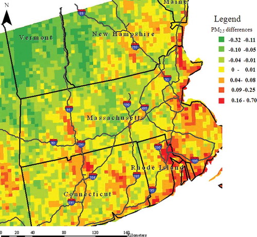
During the study period, on average 52 AOD values per grid cell were retrieved, after the data were screened for outliers (e.g., to avoid cloud contamination, shadows, and bright surfaces). Mean concentration differences varied from −0.32 to 0.50 µg m⁻³ (mean = 0.02 µg m⁻³, SD = 0.19 µg m⁻³) and were log-normally distributed. As expected, highly populated areas such as Bridgeport, New Haven, Hartford, Boston, Springfield, Providence, and Albany exhibited higher PM_2.5 levels, compared with rural areas of Vermont and southwestern New Hampshire. Furthermore, grid cells along major highways (e.g., Highways 91, 95 and 395) tend to have higher PM_2.5 concentrations, perhaps because these cells are more impacted by traffic and are also densely populated. The spatial concentration patterns observed in eastern Massachusetts were similar to those found by previous studies (Kloog et al., 2011; Lee et al., 2011) and by the mixed-effects model applied to MODIS data set during the same sampling period. It must be noted that the reported PM_2.5 spatial patterns may not be representative of the entire year of 2003 because GOES data were only available after April 24.

Discussion

Several previous studies used GOES GASP AOD as a proxy to PM_2.5 (Liu et al., 2005; 2009; Paciorek et al., 2008). For example, a two-stage generalized additive model between AOD and PM_2.5, adjusted for relative humidity and planetary boundary layer, was applied to eastern Massachusetts data and produced an R ² of 0.79 (Liu et al., 2009). Our results suggest that because the relationship between AOD and PM_2.5 varies daily, there is a need to adjust for this variability within a given domain. For the domain studied, this daily adjustment renders AOD a robust predictor of PM_2.5, with an R ² of about 0.92. These findings agree with those obtained by applying the daily adjustment approach to MODIS data (Kloog et al., 2011; Lee et al., 2011). The advantage of using GOES is its higher spatial resolution compared with that of MODIS (10 km for MODIS vs. 4 km for GOES). The improved resolution is expected to not only reduce exposure assessment error but also generally result in larger health effects estimates.

Overall, our results show that daily adjustment effectively controls for the combined effect of many parameters that can influence the daily variability in the AOD-PM_2.5 relationship. This renders our method robust and simple to use for future applications. Hoff and Christopher (2009) in their critical review recommended conducting a study to examine the effects of extrinsic factors that influence the AOD-PM_2.5 relationship separately for each region. This implies that within a given region, the types of aerosols may be more homogeneous and the height of the boundary layer and humidity may be more uniform, making the relationship between AOD and PM_2.5 less variable. Therefore, the proposed method has the advantage that it can easily be applied to other regions by taking into account the conditions prevailing in each region, and adjusting for daily variability in the AOD-PM_2.5 relationship.

The high prediction accuracy of our model confirms that the AOD-PM_2.5 relationship exhibits minimal spatial variability on a given day within the studied region comprising the states of Massachusetts, Connecticut, and Rhode Island. However, for larger regions we might encounter much larger variability in this relationship, so there would likely be a need to divide a region into subregions (e.g. to provide more homogeneous physical properties), and thus to construct a separate model for each subregion.

We also need to consider a few limitations of the methodology of the present study. The main limitation is that this approach requires a large amount of daily PM_2.5 stations, which are not always available in any given region. Therefore, the developed model would not be directly transferable for areas without sufficient EPA PM_2.5 monitors. However, typical losses of satellite AOD retrieval days do not appear to cause a similar limitation. For example, Kloog et al. (2011) successfully estimated PM_2.5 for nonretrieval days based on mixed-effects model and Land Use (LU) regression. Furthermore, Christopher and Gupta (2009) concluded that for the continental United States, cloud cover is not a major problem for inferring monthly to yearly PM_2.5 from space-borne sensors. Therefore, for epidemiological studies, such data could be used to assess both acute (short-term) and chronic (long-term) effects of PM_2.5, or combinations of acute and chronic effects.

Apart from the impact of site-specific characteristics, the differences between measured and predicted PM_2.5 levels can be attributed to errors in PM_2.5 measurements and AOD retrieval. Sources of errors in the GASP AOD retrieval include assumptions about the aerosol layer height in the radiative transfer model, the Lambertian surface assumption in the surface reflectance distribution, cloud shadows, and the clear sky composite image selected for calculating the surface reflectivity (Knapp, 2002; Knapp et al., 2005; Kondragunta et al., 2008; Prados et al., 2007). Other potential sources of uncertainty in the AOD retrieval are errors in the cloud-mask algorithm, which would lead to a high bias in the retrieved AOD. For example, errors in the AOD measurements due to clear and low-pollution days directly propagate into the precision with which PM can be estimated and therefore making this technology insufficiently robust for regulatory applications.

From the epidemiological and exposure assessment point of view, it is of high importance to have information about the spatial variability of the exposures. Because the GOES data can be used to reasonably predict the spatial patterns of PM_2.5 concentrations in the New England domain, it is possible to expand the geographic area from that used by existing epidemiological studies. Furthermore, many population exposure assessment studies have relied on city-average concentrations measured at central ground monitors. However, a city-average exposure ignores intraurban exposure contrasts and therefore might underestimate the magnitude of the association between PM_2.5 and health outcomes. Therefore, if spatially resolved data are predicted realistically, they should be superior to the existing standard data collected from one or several sites.

There are two main areas in which AOD retrievals can be improved. The first relates to spatial resolution of currently existing products, which is too coarse (e.g., 10 × 10 km for MODIS and 4 × 4 km for GOES). This limits our ability to investigate the spatial patterns of urban air quality, such as examining exposures in areas with high traffic. Future releases of higher spatial resolution of MODIS AOD retrievals (1 × 1 km) may address this limitation in part. In a recent paper, Kloog et al. (2011) applied day-specific adjustments of 10 × 10 km MODIS AOD data using ground PM_2.5 measurements and incorporated in the same model commonly used Land Use (LU) variables and meteorological variables. This made it possible to estimate the effect of traffic, elevation, or population on PM_2.5 concentrations by combining AOD and LU data. A second improvement can be achieved by increasing the retrieval accuracy in determining the microphysical and optical properties of the aerosols, which would make the retrieval of AOD or extinction more robust. In this regard, hyperspectral satellite instruments (hundreds of wavelengths) have the ability to substantially increase the accuracy in estimation of aerosol size, single scattering albedo, and indices of refraction.

In summary, in this paper we have clearly demonstrated how AOD can be used reliably to predict daily PM_2.5 mass concentrations, providing determination of their spatial and temporal variability. Promising results are found by adjusting for daily variability in the AOD-PM_2.5 relationship, without the need to account for a wide variety of individual additional parameters.

Acknowledgments

The authors wish to thank the anonymous reviewers for their constructive comments. This research was supported by a postdoctoral fellowship from the Environment Health Fund (EHF), Jerusalem, Israel. This study was funded by the Harvard EPA PM Center (R-832416), Harvard Clean Air Research Center (CLARC) (R-83479801), and the Yale Center for Perinatal, Pediatric and Environmental Epidemiology (NIH-NIEHS R01-ES-016317). Also, support was provided by NIEHS grants (ES009825 and ES00002). A.B.K.'s work was supported by the NSF grant ATM05-5467. The authors greatly appreciate advice from Dr. Joy E. Lawrence and Dr. Mike Wolfson from HSPH. The authors also thank Jeffrey Robel from the Customer Services Branch, National Climatic Data Center for providing the GASP AOD data and technical support. The authors appreciate the assistance of Steven Melley from HSPH for the GIS support and Dr. Yang Liu from Emory University, for guidance and data management in IDL.

References

- Engel-Cox , J. , Hoff , R. and Haymet , A. 2004 . Recommendations on the use of satellite remote-sensing data for urban air quality . J. Air Waste Manage. Assoc. , 54 : 1360 – 1371 .
- Engel-Cox , J. , Hoff , R. , Rogers , R. , Dimmick , F. , Rush , A. and Szykman , J. 2006 . Integrating lidar and satellite optical depth with ambient monitoring for 3-dimensional particulate characterization . Atmos. Environ. , 40 : 8056 – 8067 .
- Garrett , F. , Laird , N. and Ware , J. 2004 . Applied Longitudinal Analysis , New Jersey : Wiley & Sons .
- Gupta , P. , Christopher , S. , Wang , J. , Gehrig , R. , Lee , Y. and Kumar , N. 2006 . Satellite remote sensing of particulate matter and air quality assessment over global cities . Atmos. Environ. , 40 : 5880 – 5892 .
- Hoff , R. and Christopher , S. 2009 . Remote sensing of particulate pollution from space: Have we reached the promised land? . J. Air Waste Manage. Assoc. , 59 : 645 – 675 . doi: 10.3155/1047-3289.59.6.645
- Kaufman , Y.J. and Fraser , R.S. 1983 . Light extinction by aerosols during summer air pollution . J. Appl. Meteorol. , 22 : 1694 – 1706 .
- Kloog , I. , Koutrakis , P. , Coull , B. , Lee , H. and Schwartz , J. 2011 . Assessing temporally and spatially resolved PM2.5 exposures for epidemiological studies using satellite aerosol optical depth measurements . Atmos. Environ. , 45 : 6267 – 6275 .
- Knapp , K.R. 2002 . Quantification of aerosol signal in GOES visible imagery over the U.S . J. Geophys. Res. , 107 : 4426 doi: 10.1029/2001JD002001
- Knapp , K.R. , Frouin , R. , Kondragunta , S. and Prados , A. 2005 . Toward aerosol optical depth retrievals over land from GOES visible radiances: Determining surface reflectance . Int. J. Remote Sens. , 26 : 4097 – 4116 .
- Koelemeijer , R. , Homan , C. and Matthijsen , J. 2006 . Comparison of spatial and temporal variations of aerosol optical thickness and particulate matter over Europe . Atmos. Environ. , 40 : 5304 – 5315 .
- Kondragunta , S. , Lee , P. , McQueen , J. , Kittaka , C. , Prados , A.I. , Ciren , P. , Laszlo , I. , Pierce , R.B. , Hoff , R. and Szykman , J.J. 2008 . Air quality forecast verification using satellite data . J. Appl. Meteorol. Climatol. , 47 : 425 – 442 .
- Laird , N.M. and Ware , J.H. 1982 . Random-effects models for longitudinal data . Biometrics. , 38 : 963 – 974 . doi: 10.2307/2529876
- Lee , H.J. , Liu , Y. , Coull , B.A. , Schwartz , J. and Koutrakis , P. 2011 . A novel calibration approach of MODIS AOD data to predict PM2.5 concentrations . Atmos. Chem. Phys. , 11 : 7991 – 8002 .
- Lindstrom , M.L. and Bates , D.M. 1988 . Newton-Raphson and EM algorithms for linear mixed-effects models for repeated-measures data . J. Am. Stat. Assoc. , 83 : 1014 – 1021 .
- Liu , Y. , Paciorek , C.J. and Koutrakis , P. 2009 . Estimating regional spatial and temporal variability of PM2.5 concentrations using satellite data, meteorology, and land use information . Environ. Health Perspect. , 117 : 886 – 892 .
- Liu , Y. , Sarnat , J. , Kilaru , A. , Jacob , D. and Koutrakis , P. 2005 . Estimating ground-level PM2.5 in the eastern United States using satellite remote sensing . Environ. Sci. Technol. , 39 : 3269 – 3278 .
- Paciorek , C.J. , Liu , Y. , Moreno-Macias , H. and Kondragunta , S. 2008 . Spatiotemporal associations between GOES aerosol optical depth retrievals and ground-level PM2.5 . Environ. Sci. Technol. , 42 : 5800 – 5806 .
- Prados , A. , Kondragunta , S. , Ciren , P. and Knapp , K. 2007 . The GOES Aerosol/Smoke Product (GASP) over North America: Comparisons to AERONET and MODIS observations . J. Geophys. Res. , 112 : D15201 doi: 10.1029/2006JD007968
- Schaap , M. , Apituley , A. , Timmermans , R.M.A. , Koelemeijer , R.B.A. and de Leeuw , G. 2009 . Exploring the relation between aerosol optical depth and PM2.5 at Cabauw, The Netherlands . Atmos. Chem. Phys. , 9 : 909 – 925 .
- Wang , J. and Christopher , S.A. 2003 . Intercomparisons between satellite-derived aerosol optical thickness and PM2.5 mass: Implications for air quality studies . Geophys. Res. Lett. , 30 ( 21 ) : 2095 doi: 10.1029/2003GL018174