Evaluating the effects of climate change on summertime ozone using a relative response factor approach for policymakers

Abstract

The impact of climate change on surface-level ozone is examined through a multiscale modeling effort that linked global and regional climate models to drive air quality model simulations. Results are quantified in terms of the relative response factor (RRF_E), which estimates the relative change in peak ozone concentration for a given change in pollutant emissions (the subscript E is added to RRF to remind the reader that the RRF is due to emission changes only). A matrix of model simulations was conducted to examine the individual and combined effects of future anthropogenic emissions, biogenic emissions, and climate on the RRF_E. For each member in the matrix of simulations the warmest and coolest summers were modeled for the present-day (1995–2004) and future (2045–2054) decades. A climate adjustment factor (CAF_C or CAF_CB when biogenic emissions are allowed to change with the future climate) was defined as the ratio of the average daily maximum 8-hr ozone simulated under a future climate to that simulated under the present-day climate, and a climate-adjusted RRF_EC was calculated (RRF_EC = RRF_E × CAF_C). In general, RRF_EC > RRF_E, which suggests additional emission controls will be required to achieve the same reduction in ozone that would have been achieved in the absence of climate change. Changes in biogenic emissions generally have a smaller impact on the RRF_E than does future climate change itself. The direction of the biogenic effect appears closely linked to organic-nitrate chemistry and whether ozone formation is limited by volatile organic compounds (VOC) or oxides of nitrogen (NO_X = NO + NO₂). Regions that are generally NO_X limited show a decrease in ozone and RRF_EC, while VOC-limited regions show an increase in ozone and RRF_EC. Comparing results to a previous study using different climate assumptions and models showed large variability in the CAF_CB.

Implications:

We present a methodology for adjusting the RRF to account for the influence of climate change on ozone. The findings of this work suggest that in some geographic regions, climate change has the potential to negate decreases in surface ozone concentrations that would otherwise be achieved through ozone mitigation strategies. In regions of high biogenic VOC emissions relative to anthropogenic NO_X emissions, the impact of climate change is somewhat reduced, while the opposite is true in regions of high anthropogenic NO_X emissions relative to biogenic VOC emissions. Further, different future climate realizations are shown to impact ozone in different ways.

Introduction

In recent years, the term “climate penalty” has become a commonly used phrase to describe the negative impact that climate change may have on surface ozone concentrations and the subsequently more stringent emissions controls that would be required to meet ozone air quality standards (Jacob and Winner, 2008; Wu et al., 2008). Despite the many comprehensive modeling studies examining the potential impact of climate change on ozone (e.g., Weaver et al., 2009, summarizing work from a number of studies on the continental United States), this “climate penalty” has not yet been quantified in a way meaningful to regulators.

In the United States, state and local agencies are required to develop state implementation plans (SIPs) detailing the policies and control measures that will be implemented to bring ozone nonattainment regions into attainment with the National Ambient Air Quality Standard (NAAQS). As part of the SIP process, regulators use chemical transport models (CTMs), such as the Community Multi-scale Air Quality (CMAQ) model (Byun and Schere, 2006) and the Comprehensive Air Quality Model with extensions (CAMx; http://www.camx.com), to demonstrate that proposed control measures will lead to attainment of the ozone NAAQS.

In the 8-hr ozone SIP, U.S. Environmental Protection Agency (EPA) guidelines call for models to be used in a relative sense, where the ratio of the future to baseline (current) simulated daily maximum 8-hr ozone is calculated instead of the absolute difference between the two simulations. The future and baseline simulations typically use the same meteorology, biogenic emissions, and chemical boundary conditions, so only differ in the baseline and future control strategy anthropogenic emission inventories. The ratio of the simulated control case to baseline daily maximum 8-hr ozone at any monitor is termed a relative response factor (RRF) and represents the model response to a specific change in emissions. The RRF is typically calculated for individual days that meet specific model performance criteria, and then these daily RRFs are averaged to obtain an overall monitor-specific average RRF. To estimate the ozone concentration that would be achieved by a given change in anthropogenic emissions, the product of the average RRF and a site-specific design value (DV) ozone concentration is calculated (control ozone = average RRF × DV), where the design value is representative of observed summertime peak 8-hr ozone. If the future control ozone concentration is below the 8-hr ozone NAAQS, then the proposed emission controls are sufficient to bring the monitor into attainment (see U.S. EPA [2007] for a detailed description of how to calculate the ozone RRF and monitor design value concentration).

Since CTM modeling is such an integral component in demonstrating future attainment of the ozone NAAQS, the potential climate change impact on ozone should be quantified in a way that is useful to regulators; specifically, the impact of climate change should be accounted for in terms of the RRF. The goal of this paper is to quantify results from an ongoing multiscale modeling effort investigating the potential direct and indirect effects of global climate changes on U.S. air quality in a way that is meaningful to regulators. Results are presented in a manner that is consistent with the current use of models in the development of the ozone SIP.

Modeling

Climate and meteorology

The Weather Research and Forecasting (WRF) mesoscale meteorological model (Skamarock et al., 2005; http://www.wrf-model.org) was used to simulate both current (1995–2004) and future (2045–2054) summertime climate conditions. The WRF model is a state-of-the-science mesoscale weather prediction system suitable for a broad spectrum of applications ranging from meters to thousands of kilometers, and has been developed and used extensively for regional climate modeling (e.g., Leung et al., 2006). For this study, WRF was applied with nested 108-km and 36-km horizontal resolution domains, centered over the continental United States, with 31 vertical layers. The 108-km domain was forced with output from the ECHAM5 general circulation model (Roeckner et al., 1999, 2003) coupled to the Max Planck Institute ocean model (Marsland et al., 2003). For the current decade, ECHAM5 was run with historical forcing through 1999. From 2000 to 2004 and for the future decade, ECHAM5 was run with the Intergovernmental Panel on Climate Change (IPCC) Special Report on Emissions Scenarios (SRES) A1B scenario (Nakicenovic et al., 2000). The A1B projection assumes a balanced progress along all resource and technological sectors, resulting in a balanced increase in greenhouse gas concentrations from 2000 to the 2050s. The ECHAM5-driven WRF simulations for the current decade have been shown to represent the ENSO (El Niño–Southern Oscillation) patterns and extreme temperature and precipitation over the western United States reasonably well (Dulière et al., 2011; Zhang et al., 2011). In addition to the 108-km and 36-km simulations, WRF was also run on a 220-km horizontal resolution semi-hemispheric domain, which encompasses East Asia, the Pacific Ocean, and North America (the semi-hemispheric WRF simulations were forced by the same ECHAM5 output used in the 108-km simulations). Results from the 220-km simulations were used to drive semi-hemispheric CTM simulations, which provide chemical boundary conditions for 36-km CTM simulations over the continental United States. For details on the WRF model setup and model evaluation, the reader is referred to Salathé et al. (2010).

Chemical transport modeling and emissions

The CMAQ model version 4.7 (Foley et al., 2010), with the SAPRC99 (Carter, 2000) chemical mechanism and version 5 of the aerosol module, was used to simulate the potential impact of climate change on surface ozone over the continental United States. CMAQ simulations were conducted on two domains (Figure 1). The first, a 220-km horizontal resolution semi-hemispheric domain, captures the transport of Asian emissions to the U.S. west coast and provides chemical boundary conditions for the 36-km horizontal resolution continental U.S. (CONUS) domain. Simulations for both domains were conducted with 18 vertical layers from the surface up to 100 mbar, with a nominal depth in the surface layer of ∼40 m. Since pollution transport into the continental United States is generally dominated by Mexico emissions to the south, Canadian emissions to the north, and Asian emissions to the west, boundary conditions for the semi-hemispheric simulations were based on the default CMAQ boundary profiles. Although the use of default CMAQ boundary profiles on the semi-hemispheric domain may over-/underestimate the contribution of European emissions to continental U.S. ozone, studies have shown that this contribution is small compared to the contribution from local emission sources (e.g., Reidmiller et al., 2009). The semi-hemispheric derived boundary conditions were compared (not shown) to those of a previous study (Avise et al., 2008; Chen et al., 2009), which used a similar vertical grid structure but derived boundary conditions from MOZART global chemistry model simulations and found that they compared reasonably well throughout the boundary layer and into the upper troposphere, but showed differences in the top one to two model layers due to a lack of explicit stratospheric chemistry in CMAQ. Although CMAQ has a zero-flux boundary at the top of the modeling domain, transport from the top model layers to the surface can occur. However, the rate of vertical transport is uncertain and significant transport generally occurs only in isolated regions of complex terrain. We do not expect differences in the boundary conditions for the top model layers to have any significant impact on the findings of this work.

Figure 1. Semi-hemispheric and continental U.S. (CONUS) CMAQ modeling domains.

Meteorology for both the hemispheric and CONUS domains is based on the downscaled ECHAM5 simulations, where the future climate is represented by SRES A1B assumptions. The WRF meteorological fields were processed with the Meteorology-Chemistry Interface Processor (MCIP) version 3.4.1 (Otte and Pleim, 2010). Chemical boundary conditions (CBCs) for the CONUS domain were provided by the semi-hemispheric CMAQ simulations. For all simulations, biogenic emissions were estimated using the Model of Emissions of Gases and Aerosols from Nature version 2.04 (MEGANv2.04; Guenther et al., 2006; http://cdp.ucar.edu) using meteorological output from MCIP and the default MEGANv2 land cover data. Land use and land cover (LULC) were held constant at current decade conditions for all simulations. This version of MEGAN does not account for the impact that rising atmospheric carbon dioxide (CO₂) concentrations have on biogenic isoprene emissions, which will likely lead to an overestimate of the increase in biogenic emissions expected under a warmer future climate (Heald et al., 2009).

Anthropogenic emissions of reactive gaseous species for the semi-hemispheric domain were from the POET (Granier et al., 2005; Olivier et al., 2003) and EDGAR (European Commission, 2010) global inventories; organic and black carbon emissions were from Bond et al. (2004). Current anthropogenic emissions for the CONUS domain were based on the U.S. EPA National Emissions Inventory for 2002 (NEI2002; http://www.epa.gov/ttnchie1/net/2002inventory.html). These emissions were projected to 2050 using the Emission Scenario Projection version 1.0 (ESP v1.0; Loughlin et al., 2011) methodology, which is based on the MARKet ALlocation (MARKAL) model (Fishbone and Abilock, 1981; Loulou et al., 2004; Rafaj et al., 2005) coupled to a database developed by the U.S. EPA, which represents the U.S. energy system at national and regional levels (U.S. EPA, 2006). The future-decade emissions were based on a business-as-usual scenario, where current emissions regulations are extended through 2050 (“Scenario 1” in Loughlin et al., 2011). Future MARKAL emission estimates were used, rather than SRES A1B estimates, because the MARKAL estimates provide a more detailed and realistic projection of future U.S. emissions. The MARKAL version used in this work did not provide full coverage of energy sector pollutant species, so the growth factors for CO₂ were used as surrogates for growth in carbon monoxide (CO), nonmethane volatile organic compound (NMVOC), and ammonia (NH₃) emissions, while the PM₁₀ (PM with aerodynamic diameter less than 10 μm) growth factors were applied to PM_2.5 (PM with aerodynamic diameter less than 2.5 μm). For mobile source emissions, growth factors for oxides of nitrogen (NO_X = NO + NO₂) were used to project CO, NMVOC, and NH₃ emissions. The business-as-usual scenario includes an approximation of the Clean Air Interstate Rule limits on electric-sector sulfur dioxide (SO₂) and NO_X emissions; a requirement that all new coal-fired power plants utilize low-NO_X burners and select catalytic reduction and flue gas desulfurization controls; heavy-duty-vehicle emission limits on SO₂, NO_X, and particulate matter (PM); Tier II emission limits and fleet efficiency standards for light duty vehicles; and implementation of the renewable fuel standards targets of the Energy Independence and Security Act of 2007.

Percent changes in modeled anthropogenic and biogenic emissions for the CONUS domain are shown in Figure 3. Emissions are summarized for the regions defined in Figure 2. Under the MARKAL 2050 business-as-usual scenario, emissions of NO_X and SO₂ are projected to decrease in all regions. The decrease in NO_X emissions ranges from 16% in the South to 35% in the Northeast, while the decrease in SO₂ emissions is greatest in the Northwest (35%) and least in the Southwest (16%). Anthropogenic emissions of CO, NMVOCs, NH₃, and PM_2.5 are projected to increase across all regions. Increases in CO range from 7% in the South to 70% in the Midwest. Emissions of NMVOCs also show the smallest increase in the South (13%), with the largest increase occurring in the Central region (33%). The increase in ammonia emissions is relatively constant across all regions (33–39%), while increases in PM_2.5 emissions range from 2% in the Central region to 22% in the Northwest. Emissions of biogenic VOCs (BVOCs) closely follow the simulated change in temperature (discussed in the Simulated Climate Change section) and show an increase in all regions except the Northwest, which experiences a slight decrease in BVOC emissions due to a projected decrease in the temperature of that region. As mentioned earlier, the increase in BVOC emissions for most regions is likely overestimated since we did not account for the effects of rising levels of CO₂ in the atmosphere (Heald et al., 2009).

Figure 2. Definition of the regions used in summarizing results.

Figure 3. Percent change in continental U.S. emissions from the present-day to the 2050s by region. BVOC represents biogenic VOC emissions that are allowed to change with the future climate.

Simulations

Six sets of simulations were conducted to examine the separate and combined effects of projected climate and U.S. anthropogenic emission changes on ozone and the RRF. A summary of the simulations performed for this study is provided in Table 1. Simulation CD_Base represents the base case in which all variables are kept at the present-day conditions. FD_US is the same as CD_Base, except that U.S. anthropogenic emissions are at 2050s levels. A1B_Met is the same as CD_Base, except that future-decade instead of current-decade meteorology is used to drive the CMAQ simulations (future meteorology impacts atmospheric transport and chemical reactions rates, but not biogenic emissions). A1B_M is the same as A1B_Met, except that future meteorology is also used to drive MEGAN to derive future-decade biogenic emissions. The last two sets of simulations involve the combined effects of projected climate and U.S. anthropogenic emissions changes. A1B_US_Met uses future meteorology and U.S. anthropogenic emissions with biogenic emissions held at current-decade levels. A1B_US_M is the same as A1B_US_Met, except that biogenic emissions are based on future-decade meteorology.

Table 1. Matrix of 36-km CONUS domain CMAQ simulations

Simulation name	Meteorology	Anthropogenic emissions	Biogenic emissions
CD_Base	Current	NEI 2002	Current meteorology
FD_US	Current	MARKAL 2050	Current meteorology
A1B_Met	Future	NEI 2002	Current meteorology
A1B_M	Future	NEI 2002	Future meteorology
A1B_US_Met	Future	MARKAL 2050	Current meteorology
A1B_US_M	Future	MARKAL 2050	Future meteorology
Note: Future meteorology is based on the IPCC A1B scenario. NEI 2002 refers to the U.S. EPA National Emissions Inventory for 2002. MARKAL 2050 refers to a future emissions inventory that is based on the NEI 2002 and projected to 2050 using the U.S. EPA MARKAL allocation model. The same present-day chemical boundary conditions from the semi-hemispheric CMAQ simulations are used for all cases. All simulations use present-day land-use and land-cover data. Chemical boundary conditions are held constant at present-day levels for all simulations.

Each simulation was conducted for two sets of summer climatology (June, July, August), representing the warmest and coldest summers (based on the mean surface temperature across the United States) within the current (1995–2004) and future (2045–2054) decades. Chemical boundary conditions are held constant at present-day levels for all simulations and are based on the 220-km semi-hemispheric domain CMAQ simulations using present-day meteorology and anthropogenic emissions. Present-day LULC data are applied to all simulations. Wildfire emissions are not included in the simulations due to the uncertainty in predicting future fires. We will address the effect of changes in projected future wildfire emissions on surface ozone and PM in a future paper.

Results and Discussion

Simulated climate change

Changes in climate can have both direct and indirect effects on ozone levels. Direct effects include enhanced photochemistry through increases in temperature and insolation, improved ventilation from increases in wind speed and planetary boundary layer (PBL) heights, removal of pollutants from the atmosphere through precipitation, and a reduction in background ozone from increased water vapor content (Jacob and Winner, 2008, and references therein). Indirect effects include changes in temperature-sensitive emissions from biogenic sources, as well as climate-induced relocation of those sources through plant species migration (Cox et al., 2000; Sanderson et al., 2003). Percent change in ozone-relevant meteorological parameters from the 36-km WRF simulations are shown in Figure 4. Results are averaged over the seven regions defined in Figure 3. Changes in meteorological parameters were calculated from averages of the warmest and coldest summers in each decade, which correspond to the summers used in the CMAQ simulations. For temperature and boundary layer height, changes in the average daily maximum are shown, while for water vapor, precipitation, insolation, and wind speed, changes in the average values are shown.

Figure 4. Simulated change in meteorological parameters due to climate change. Percent change in temperature (˚C) and PBL are from average daily maximum values, while water vapor, precipitation, insolation, and wind speed are from average values.

On average, the change in temperature (shown as percent ˚C) tends to increase from west to east across the United States, with the largest temperature increase occurring in the Northeast (15%) and the only decrease in temperature occurring in the Northwest (1%). The same general west-to-east trend is also seen with other meteorological parameters. PBL height increases in all regions, with the smallest increase occurring in the Northwest and Southwest (3–4%) and a relatively constant increase in the other regions (10–12%). Insolation decreases slightly in the Northwest (4%) but increases in all other regions, peaking in the Northeast at 8%. Water vapor content shows the largest decrease in the Southwest (7%), with only slight decreases in the Northwest and Central regions. All other regions show an increase in water vapor content, with the largest increases occurring in the Northeast (8%) and Southeast (7%). In contrast to the other meteorological parameters, wind speed and precipitation do not show a west to east trend. Changes in wind speed vary from a decrease of 2–4% in the Northwest and Southeast to an increase of 5% in the Southwest and Central regions. Precipitation is predicted to decrease in all regions and ranges from 1% in the Southeast to greater than 50% in the Southwest.

The results presented in Figure 4 are generally consistent with published results from other studies simulating a future 2050 A1B climate. For example, Leung and Gustafson (2005) simulated a current (1995–2005) and future (2045–2055) A1B climate using the MM5 mesoscale meteorological model (Grell et al., 1994) driven by the Goddard Institute of Space Studies (GISS) global climate model (Rind et al., 1999). The work of Leung and Gustafson (2005) has been widely used in modeling studies examining the impact of climate change on air quality (Liao et al., 2009; Tagaris et al., 2007; Zhang et al., 2008). Although their work is based on the same A1B scenario as the results presented here, differences do arise because of the use of different global and mesoscale models and the choice of current and future years to simulate (e.g., some years may be warmer or colder than others). The most notable differences occur in the Northwest, where Leung and Gustafson (2005) show an increase in both temperature and precipitation, while our work shows a decrease in both parameters. These differences may be attributed to the number of years simulated; our WRF simulation results also show an increase in temperature if 10 years of simulations are included in each of the 2000 and 2050 decades (results not shown). Additional differences can be seen from Zhang et al. (2008), who use a two-year subset of meteorology from Leung and Gustafson (2005). The differences seen in Zhang et al. (2008) include an increase in precipitation in the Northwest, increased wind speed in the Southeast, and a decrease in PBL height in both the Northwest and Southwest, all of which are in contrast to the work presented here. We point out these differences to illustrate that although the work presented here is generally consistent with other similar studies, it does represent only a single future climate realization, and the use of different models, number of years simulated, and assumptions about future emissions will all result in a different future climate realization.

Ozone and climate

Elevated ozone concentrations in polluted environments are closely linked to temperature (Sillman and Samson, 1995; Wunderli and Gehrig, 1991). Although the exact mechanism relating temperature and elevated ozone may vary by region, it is likely due to a combination of the following: temperature-dependent chemical rate constants, the relationship between stagnation events and temperature, changes in meteorological parameters associated with elevated temperatures (e.g., insolation and water vapor), and temperature-dependent emissions (e.g., biogenic emissions).

Figure 5 depicts the observed and modeled relationship between summertime (June, July, August) daily maximum temperature and daily maximum ozone at 72 rural sites within the Clean Air Status and Trends Network (CASTNET; http://www.epa.gov/castnet). Observations are from 1998–2002, and model results are from the two summers representing the warmest and coldest simulated summers from the current decade (CD_Base case). Observations beyond 2002 are not considered because the large reduction in power plant NO_X emissions in the eastern United States that occurred around 2002 is not reflected in the NEI2002 emission inventory.

In general, the modeled ozone and temperature fall within the range of observed values in each region. However, the modeled results do not show the same day-to-day variability as seen in the observations. This is not unexpected, since five years of observations are used, compared to two modeled years, and because the model results are averaged over a 36-km grid-cell whereas the observations represent measurements at a single point in space. The average ozone–temperature relationship can be represented by the slope of the linear best-fit. The slopes of the modeled and observed linear best-fit for each region are within approximately ±15% of each other, except for in the Central and Southeast regions. These two regions show only minor ozone correlation to temperature, suggesting either that temperature is not the main driver for peak ozone at the CASTNET sites within those regions, or that temperature at these sites is less correlated to other mechanisms that drive elevated ozone, such as stagnation events. The ozone–temperature relationship shown in Figure 5 is generally consistent with the pre-2002 results of Bloomer et al. (2009), but the slopes of the observed linear best-fit do not match exactly since Bloomer et al. (2009) included additional years (1987–2002) in their analysis, grouped sites in a slightly different manner, and used all hourly data rather than the daily maximum hourly values used in this work.

Figure 5. Observed (open dark circles) and modeled (open gray circles) daily maximum hourly ozone as a function of summertime daily maximum hourly temperature at 72 CASTNET sites. The data have been grouped by site location based on the region definitions in Figure 2. The observed and modeled linear best-fit lines are shown as solid and dashed, respectively. The slope of the linear best-fit is shown in the upper-left corner of each tile [ppb/˚C].

Based on the ozone–temperature relationship, under a warmer future climate, ozone would be expected to increase. This relationship generally holds true for the projected change in temperature and ozone between the current- (CD_Base) and future-climate (A1B_Met) simulations (Figure 6). In regions where temperature is projected to increase under a future climate, ozone is also projected to increase, while in the Northwest, where future temperature is projected to decrease, ozone also decreases. The same trend is seen when biogenic emissions are allowed to change with the future climate (A1B_M case).

Figure 6. Simulated change in average daily maximum temperature and the corresponding change in average daily maximum 1-hr ozone at the 72 CASTNET sites when biogenic emissions are held constant (A1B_Met; solid circles) and when biogenic emissions are allowed to change in response to the future climate (A1B_M; open squares).

Although the ozone–temperature relationship is useful for developing a qualitative description of how ozone may change under a future climate, it is not sufficiently robust for use by policymakers when determining the combined effects of both anthropogenic emission reductions and climate change on ozone levels. In particular, observations (Bloomer et al., 2009) and modeling studies (Wu et al., 2008) suggest that the penalty associated with climate change decreases when NO_X emissions are reduced. More recent work also suggests that the climate change penalty may be reduced at extreme high temperatures (>39°C), due to a diminishing effect of a reduced PAN (peroxyacetyl nitrate) lifetime on ozone chemistry at these temperatures (Steiner et al., 2010).

Relative Response Factor (RRF)

Previous modeling studies examining the potential effects of future climate change on ozone in the United States typically quantify their results as a change in some peak summertime ozone metric (Avise et al. 2008; Chen et al. 2008; Hogrefe et al., 2004; Racherla and Adams, 2008; Tagaris et al., 2007; Tao et al. 2007) or examine how climate change may affect ozone-relevant meteorological phenomena such as the frequency and duration of stagnation events (Leung and Gustafson, 2005; Mickley et al., 2004). Although these types of analyses provide some information to policymakers about how climate change may affect the success of ozone mitigation strategies, they do not address the issue in a way that is consistent with how models are used in regulatory applications. Specifically, they do not address how to account for the impact of climate change on ozone in terms of the RRF (i.e., how to adjust the RRF to reflect the climate penalty).

In other work, Liao et al. (2009) applied the Decoupled Direct Method 3-D (Dunker et al., 2002; Yang et al., 1997) in CMAQ to quantify the sensitivity of ozone and PM_2.5 to changes in precursor emissions under a high-extreme and low-extreme future 2050s A1B climate, where the extremes are based on the 0.5th and 99.5th percentiles of temperature and absolute humidity from the MM5 meteorological fields of Leung and Gustafson (2005); Liao et al. (2009) found that ozone sensitivity to a reduction in NO_X emissions was generally enhanced under the high-extreme climate case and reduced under the low-extreme case. They attributed the change in model response to changes in temperature-dependent biogenic emissions, which accompany the change in climate (i.e., increases in biogenic VOC emissions due to a warmer climate lead to a more NO_X-limited environment, making NO_X controls more effective at reducing ozone). Although the work by Liao et al. (2009) provides useful information for how the sensitivity of modeled ozone response to emission reductions may change under a future climate, they do not directly address how to account for the influence of climate change on ozone in the context of the RRF. In the analysis that follows, we present results in the context of the RRF and outline a methodology for adjusting the RRF to account for climate change effects on ozone.

For the purpose of this work, we define the non-climate-adjusted RRF (RRF_E) as follows, with the understanding that this is not identical to the rigorous RRF calculation described in the U.S. EPA Attainment Modeling Guidance (U.S. EPA, 2007), and that RRF_E would be replaced by an actual RRF if the following analysis were included in an ozone SIP:

(1)

where N _exc is the number of days that exceed the 8-hr ozone NAAQS (75 ppb was used in this work) in the current emissions simulation (CD_Base case), t is the day, and [O₃] is the daily maximum 8-hr ozone for days in which the current emissions simulation (CD_Base case) exceeds the 8-hr ozone NAAQS. The choice of days to include in the RRF calculation is based on the current emissions case only. Since the CD_Base and FD_US simulations use the same meteorology, eq (1) is consistent with how the RRF is applied in SIP analysis. Typically, additional day-specific model performance criteria (such as thresholds for normalized mean error and bias) are applied to the modeled data, and only days that meet these additional criteria are used in the RRF calculation (for details see U.S. EPA, 2007). However, since the meteorology used in this work is constrained by global climate model output and does not represent a specific day or time, performance statistics are not calculated. In the remainder of this paper, the term RRF refers to a general RRF that may or may not have been adjusted to account for climate change and changes in biogenic emissions. The term RRF_E refers to the RRF defined in eq (1), which has not been adjusted to account for climate change. Climate-adjusted RRFs are defined in the next section.

Figure 7 shows RRF_E at 1135 ozone monitoring locations throughout the continental United States. Modeled ozone was originally analyzed at 1199 sites with continuous monitoring records from 1995 to 2004 based on data obtained from the U.S. EPA Air Quality System database (http://www.epa.gov/ttn/airs/airsaqs/); however, 64 of the 1199 sites did not have a single day where the CD_Base case daily maximum 8-hr ozone was greater than 75 ppb, and those sites are excluded from Figure 7. Values of RRF_E less than one are shown in shades of blue and imply a reduction in ozone due to the projected anthropogenic emission changes shown in Figure 3, while values of RRF_E greater than one are shown in shades of red and imply an increase in ozone. Results are summarized by region in Table 2. Nearly all sites (97%) have an RRF_E less than one, which means ozone is reduced in nearly all locations based on the future 2050s emissions. The remaining 3% of the sites that have an RRF_E > 1 are primarily located in large urban regions with high NO_X emissions that are known to exhibit an ozone disbenefit to NO_X reductions, such that ozone increases with decreasing NO_X emissions. It should be noted that even in these disbenefit regions, if NO_X emissions continue to decrease, at some point there will no longer be a disbenefit and ozone will decrease with a continued reduction in NO_X emissions.

Table 2. Summary of RRF_E by region

		RRFE
Region	Number of sites	Average	Minimum	Maximum	Standard deviation	Percent of sites with RRF >1.00
Northwest	11	0.95	0.92	0.97	0.021	0
Southwest	246	0.91	0.85	1.07	0.043	5
Central	31	0.92	0.86	0.98	0.030	0
South	124	0.95	0.88	1.02	0.040	9
Midwest	287	0.95	0.91	1.00	0.019	0
Southeast	211	0.91	0.84	0.99	0.027	0
Northeast	225	0.92	0.85	1.16	0.048	3
All regions	1135	0.93	0.84	1.16	0.040	3

Figure 7. Spatial map of the RRF_E for the 1135 ozone monitoring locations in which the CD_Base case had at least one day where the daily maximum 8-hr ozone exceeded 75 ppb. Values less than one imply a reduction in daily maximum 8-hr ozone, while values greater than one imply an increase in daily maximum 8-hr ozone when anthropogenic emissions are reduced as shown in Figure 3 (color figure available online).

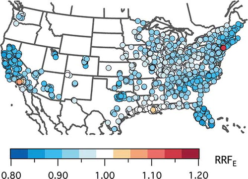
In calculating the RRF_E a low threshold was used, where a site required only a single day with daily maximum 8-hr ozone greater than 75 ppb to calculate an RRF_E, in order to maximize the number of sites used in the analysis. Although using a higher threshold may result in a more stable RRF_E, it would also reduce the number of sites, as well as the spatial coverage of those sites. In regions with high ozone and many sites (Southwest, South, Midwest, Southeast, and Northeast regions), the low threshold has little impact on the results compared to a higher threshold. However, in regions with lower ozone and fewer sites (Northwest and Central regions), using a higher threshold can significantly reduce the number of sites included in the analysis. For example, if a threshold of five days is used instead of one day (not shown), there will be no sites in the Northwest for which an RRF_E can be calculated and the number of sites in the Central region will drop from 31 to 9. The number of sites in other regions decreases much less (∼20% or less) and the results in these regions are not affected.

Adjusting the RRF to Account for Climate Change

A key issue facing regulatory agencies is how to account for the potential impact of climate change on ozone within the guidelines of a SIP. One possible methodology is to adjust the RRF to account for climate change effects. This is advantageous because it builds from of the RRF analysis currently called for in the development of the ozone SIP. We do this in terms of a climate adjustment factor (CAF) and define two CAFs as follows:

(2)

(3)

where N _all is the number of simulation days, t is the day, and [O₃] is the daily maximum 8-hr ozone. CAF_C only accounts for changes in climate, while CAF_CB accounts for changes in both climate and biogenic emissions. Climate adjusted RRFs can then be defined as

(4)

(5)

where RRF_E is defined in eq (1), CAF_C is defined in eq (2), and CAF_CB is defined in eq (3). Equations (4) and (5) are used to adjust RRF_E in Figure 7 and Table 2. Results for RRF_ECB are shown in Figure 8 along with the CAF_CB, and summarized in Table 3 for RRF_EC and RRF_ECB.

Table 3. Summary of climate-adjusted RRFs ( eqs (4) and (5)) by region

		RRFEC (RRFECB)
Region	Number of sites	Average	Minimum	Maximum	Standard deviation	Percent of sites with RRF >1.00
Northwest	11	0.87	0.84	0.89	0.020	0
		(0.87)	(0.84)	(0.89)	(0.017)	(0)
Southwest	246	0.91	0.82	1.09	0.059	7
		(0.92)	(0.83)	(1.15)	(0.070)	(13)
Central	31	0.97	0.88	1.07	0.066	42
		(0.98)	(0.87)	(1.10)	(0.074)	(42)
South	124	1.04	0.94	1.16	0.057	66
		(1.05)	(0.94)	(1.22)	(0.071)	(65)
Midwest	287	1.04	0.97	1.13	0.033	89
		(1.05)	(0.94)	(1.18)	(0.047)	(88)
Southeast	211	0.99	0.85	1.07	0.039	31
		(0.97)	(0.85)	(1.11)	(0.040)	(22)
Northeast	225	1.00	0.91	1.25	0.057	32
		(1.00)	(0.90)	(1.34)	(0.074)	(30)
All regions	1135	0.99	0.82	1.25	0.069	45
		(1.00)	(0.83)	(1.34)	(0.079)	(43)

Figure 8. Climate adjustment factor (CAF_CB) for the A1B_US_M case (top), and the associated climate adjusted RRF (RRF_ECB; bottom). A CAF is calculated for all sites, but not all sites have an RRF (color figure available online).

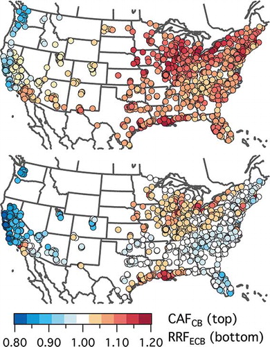
In all regions, except the Northwest and Southwest, climate change increases the regional average RRF, the peak RRF, and the spatial variability (represented by the standard deviation) of the RRF (i.e., RRF_EC > RRF_E). In the Southwest, the peak RRF and the spatial variability of the RRF both increase under future climate conditions (RRF_EC > RRF_E), while the average RRF is unchanged (RRF_EC ≈ RRF_E). In the South, Midwest, and Northeast, the increase in the average RRF due to climate change is sufficient to more than offset the decrease in ozone achieved by the change in anthropogenic emissions (i.e., RRF_E < 1 ≤ RRF_EC). In other regions, the increase in RRF due to climate change does not completely offset the decrease in ozone achieved by the projected anthropogenic emission changes, but it does reduce the effect those changes have on ozone (i.e., RRF_E < RRF_EC < 1). In all regions but the Northwest, the number of sites having an RRF_EC > 1 greatly increases under the future climate, with nearly half (45%) of all sites having an RRF_EC > 1 (Table 3), compared to only 3% when climate change is not accounted for (RRF_E; Table 2). The increase in the RRF under the future climate is consistent with other studies that attribute the increase in ozone to enhanced PAN decomposition at higher temperatures and to the association of higher temperatures with stagnation events (Jacob and Winner, 2008; Jacob et al., 1993; Sillman and Samson, 1995).

The Northwest, which is predicted in these simulations to cool under the future climate, is the only region that shows a decrease in RRF (RRF_EC < RRF_E). However, this is an artifact of the choice of summers used in this work. As previously stated, the coolest and warmest summers from each decade were chosen based on the mean surface temperature across the continental United States, which does not necessarily reflect the coolest and warmest summers in the Northwest. An examination of the change in average temperature across all 10 years in the current and future decades (not shown) found that, on average, the Northwest is expected to experience a slight increase in temperature in the future. Consequently, if all 10 summers in each decade were modeled, it is likely that an increase in the RRF would also be seen in the Northwest.

Although the effect of climate change on the RRF is generally greater than the impact of associated changes in biogenic emissions (Tables 2 and 3), the impact of biogenic emission changes is nontrivial. In the Northwest, the future climate is predicted to cool, resulting in a decrease in biogenic emissions, which has little impact on the RRF (RRF_EC ≈ RRF_ECB). For all other regions, accounting for changes in both climate and biogenic emissions generally results in a minimal increase in the regional average RRF, and a larger, more pronounced increase in the regional maximum RRF compared to the climate change only case (RRF_EC < RRF_ECB). The spatial variability of the RRF (represented by the standard deviation) also increases with enhanced biogenic emissions. In contrast, the number of sites having an RRF > 1 decreases in all regions except the Southwest, Northwest, and Central regions when biogenic emission changes are included. In the Northwest, there is no change because biogenic emissions decrease with decreasing temperature. In the Central region, both biogenic and anthropogenic emissions are relatively low to begin with, so an increase in biogenic emissions does not lead to an increase in the number of sites with an RRF > 1. In the Southwest, the number of sites with an RRF > 1 nearly doubles when biogenic emissions are allowed to change (from 7% of sites to 13%). The majority of the additional sites in the Southwest with an RRF > 1 are located in Southern California, which is known to be largely VOC limited (Harley et al., 1993; Milford et al., 1989), so an increase in biogenic VOC emissions results in an increase in ozone production.

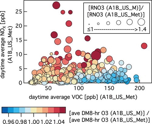
Overall, the change in the RRF to increases in biogenic emissions (RRF_EC vs. RRF_ECB) appears closely linked to VOC–nitrate chemistry and whether a region is NO_X limited or VOC limited. Although the SAPRC99 chemical mechanism used in this work does recycle NO_X from organic nitrates (RNO₃), the recycling does not occur instantaneously nor is all of the NO_X recycled. As a result, when biogenic emissions increase, the corresponding increase in peroxy radicals (HO₂ + RO₂) leads to enhanced formation of organic nitrates (RO₂ + NO ← RNO₃) and an increase in simulated RNO₃ concentrations. In regions that are generally NO_X limited (such as much of the Southeast) the enhanced formation of RNO₃ associated with increases in biogenic emissions reduces the amount of NO_X available to participate in ozone formation, resulting in a decrease in ozone. In contrast, regions such as Southern California in the Southwest, which are generally VOC limited and exhibit an ozone disbenefit to NO_X reductions, experience an increase in ozone when biogenic VOCs increase. This is due to a combination of NO_X being removed from the system through enhanced RNO₃ formation and a reduction in the scavenging of ozone by NO (HO₂ + NO ← HO + NO₂ becomes the preferred pathway for converting NO to NO₂ over the O₃ + NO ← O₂ + NO₂ pathway). This is illustrated in Figure 9, which shows average daytime NO_X as a function of average daytime VOC for the A1B_US_Met case. Data points are color coded by the ratio of average daily maximum 8-hr (ADM8-hr) ozone from the A1B_US_M case to the A1B_US_Met. Shades of red imply an increase in ADM8-hr ozone when biogenic emissions are allowed to change with climate, and shades of blue represent a decrease in ADM8-hr ozone. In regions with low NO_X and high VOC concentrations ADM8-hr ozone is reduced with future biogenic emissions, while in regions of high NO_X and/or lower VOC concentrations ADM8-hr ozone increases with future biogenic emissions.

Figure 9. Simulated average daytime NO_X as a function of average daytime VOC at ozone monitoring sites for the A1B_US_Met case. Data points are color coded based on the ratio of the average daily maximum 8-hr O₃ from the A1B_US_M and A1B_US_Met cases. The size of each data point represents the ratio of average daytime organic nitrates (RNO₃) concentration in the A1B_US_M and A1B_US_Met cases (color figure available online).

Although we have shown that changes in biogenic emissions can influence the CAF, this work does not consider CO₂ suppression of isoprene emissions under a future climate or the potential impact of changes in LULC on biogenic emissions. In particular, Heald et al. (2009) showed that projected increases in biogenic isoprene emissions as the result of a warmer climate may be offset by the suppression of those emissions due to increasing CO₂ levels in the future atmosphere. Potential changes in LULC (e.g., expansion of agricultural lands and reforestation) have also been shown to significantly impact projected biogenic emissions (Chen et al., 2009). Consequently, the impact of changes in biogenic emissions on the CAF is likely to be reduced due to CO₂ suppression, and could be reduced or enhanced depending on the effect of the projected change in LULC on biogenic emissions (e.g., expansion of crop lands into oak woodlands would result in reduced isoprene emissions).

It is important to note that we have limited our analysis to sites for which we have calculated an RRF_E (i.e., sites that had at least one day where the CD_Base case simulated a DM8-hr ozone >75 ppb). However, it is possible that climate change could push sites that are currently below the 75-ppb threshold to exceeding the threshold, and any regulatory analysis using the CAF approach should consider this possibility with regard to sites that are currently in attainment of the ozone standard.

Alternate CAF methodology

Although eqs (4) and (5) provide a straightforward methodology for adjusting the RRF to account for potential climate change effects, the application of the CAF in eqs (2) and (3) may not be a practical approach for policymakers since the future anthropogenic emission scenario would have to be known prior to the future-climate air quality simulation. Due to the time constraints involved with the development of a SIP, the future-climate air quality simulations would likely need to be completed prior to the future year emission inventory being finalized. Therefore, an alternative approach would be to calculate the CAF using current anthropogenic emissions rather than future emissions (i.e., replacing the A1B_US_Met /A1B_US_M and A1B_US simulations in eqs (2) and (3) with the A1B_Met/A1B_M and CD_Base simulations, respectively). This way, the impact of climate change as quantified by the CAF can be estimated independent of future anthropogenic emission scenarios. Figure 10a compares CAF_C and CAF_CB calculated using future anthropogenic emissions to those calculated using current anthropogenic emissions. With regard to ozone formation, the primary difference between the current and future anthropogenic emission inventories is reduced NO_X emissions in the future inventory. For both CAF_C > 1 and CAF_C < 1, decreasing NO_X emissions reduces the impact of climate change on ozone (CAF becomes closer to 1.0), which is consistent with the findings of Bloomer et al. (2009) and Wu et al. (2008), who found that the penalty associated with climate change is reduced as NO_X emissions decrease. For the future climate and anthropogenic emission scenario, the change in the CAF_C is generally small, and using a current anthropogenic emission inventory in the CAF_C calculation gives a reasonable approximation to the future anthropogenic emission CAF_C. However, regulators need to be aware that this may slightly overestimate the climate change impact in terms of the RRF. When changes in biogenic emissions are accounted for in the CAF calculation (CAF_CB), the same trends are seen but become slightly more pronounced.

Figure 10. (a) Comparison between CAF_C and CAF_CB ( eqs (2) and (3)), when future anthropogenic emissions are used (A1B_US_M and A1B_US_Met cases), and when current anthropogenic emissions are used (A1B_M and A1B_Met cases). (b) Comparison between RRF_E from eq (1) when the RRF is calculated under the current climate (CD_Base and FD_US cases) and under the future climate (A1B_Met or A1B_M and A1B_US_Met and A1B_US_M cases, respectively).

Climate impacts on the RRF

The CAF approach provides a way to account for the influence of climate change on ozone (i.e., the climate penalty) in terms of the RRF. However, this approach assumes that the RRF is independent of climate change and itself does not change under a future climate. To examine the sensitivity of the RRF to a changing climate, we calculated a new RRF following eq (1), but using results from future climate cases (i.e., replacing the CD_Base case with the A1B_Met or A1B_M cases and the FD_US case with the A1B_US_Met or A1B_US_M cases, respectively), and compared the new RRF to the original RRF from eq (1) (Figure 10b). The majority of sites (90%) had an RRF that changed less than ±0.02 when biogenic emissions were held at present-day levels; when biogenic emissions were allowed to change with the future climate, that number dropped to 84% of sites. The largest change in a single RRF occurred when biogenic emissions were allowed to change (–0.31), but generally the peak changes were within ±0.12. The overall bias was less than –0.0006 for both cases, suggesting that while climate change can have a large impact on the RRF at select sites, for the majority of sites the impact is small.

Other climate scenarios

In this work, we examined the impact of a single future climate realization on the RRF; however, the use of different climate realizations can lead to very different results. To illustrate this point, we compare results from a previous modeling study conducted by the authors that also examined the impact of climate change on U.S. air quality. Avise et al. (2008) and Chen et al. (2009) simulated current (1990–1999) and future (2045–2054) ozone over the continental United States for five summers (July only) within each decade. The five Julys were chosen to reflect the range of simulated surface temperatures across the continental United States within each decade. The most relevant differences between their work and the work presented here is in the future climate assumptions (SRES A2 vs. SRES A1B), global climate model (Parallel Climate Model vs. ECHAM5), and regional meteorological model (MM5 vs. WRF) used to simulate the future climate. Although the SRES A2 and A1B assumptions are different, the two emission scenarios do not begin to diverge significantly until the mid-21st century (Salathé et al., 2010), so the difference in future emissions scenario used to drive the global climate models should have a minor impact compared to the differences in the global climate and regional meteorological models used, as well as the specific years simulated. There is also a difference in current emission scenario between the two studies (NEI 1999 vs. NEI 2002), but the inventories are sufficiently similar that this difference should have a minimal impact compared to the differences mentioned earlier.

Figure 11 compares the CAF, using current anthropogenic emissions, calculated from the work presented here and a similarly calculated CAF from the work of Avise et al. (2008: CURall and futMETcurLU cases) and Chen et al. (2009: Cases 1 and 2). In both studies, biogenic emissions were allowed to change with the future climate and LULC values were held constant at current decade conditions. The comparison shows large differences in the CAF calculated from the two studies, and these differences occur across all regions. Detailed analysis as to why the differences in CAF occur is beyond the scope of this work. However, we show this comparison as a way of illustrating to the regulatory community the importance of considering multiple future climate realizations in any decision-making process.

Figure 11. Comparison of the climate adjustment factor (CAF_CB) from this study with that calculated from the work of Avise et al. (2008) and Chen et al. (2009), when current anthropogenic emissions are used and biogenic emissions are allowed to change with the future climate (i.e., alternate CAF methodology is used).

Conclusion

Results from a comprehensive multiscale modeling study investigating the potential impact of global climate change on summertime ozone in the United States were analyzed. The results are presented in a manner that is consistent with how air quality models are used in the development of state implementation plans (SIPs). We defined a climate adjustment factor (CAF) as the ratio of the simulated average daily maximum 8-hr ozone from a simulation using future meteorology to one using current meteorology. The CAF is used to adjust the policy-relevant relative response factor (RRF) to account for the impact that a changing climate may have on the effectiveness of emission control strategies for reducing ozone (i.e., the climate penalty). Although the climate adjusted RRF shows some regional differences, the general trend is toward an increase in the RRF when it is adjusted to account for climate change effects. This trend implies additional emission controls will be required to achieve the same reduction in ozone as would have been achieved in the absence of climate change. Changes in biogenic emissions have less of an impact than climate change itself, and the impact appears closely linked to organic-nitrate chemistry and to whether a region is NO_X limited or VOC limited. In both cases, an increase in BVOC emissions enhances organic-nitrate formation, which removes NO_X from the system. In VOC-limited regions such as Southern California, which exhibit an ozone disbenefit to NO_X emission reductions, removing NO_X from the system results in an increase in ozone. In contrast, in NO_X-limited regions such as much of the Southeast, removing NO_X through enhanced organic-nitrate formation leads to a reduction in ozone. In addition, we compared our results to a previous study (Avise et al., 2008; Chen et al., 2009) and found large variability in the CAF, which illustrates the necessity for policymakers to consider multiple future climate realizations to inform their decisions.

Although we have presented our results in a manner that is consistent with how models are used for SIP purposes, there are several differences that should be mentioned. Due to the computational demands required to conduct long-term simulations over the continental United States, it was necessary to use a 36-km horizontal grid resolution. However, most SIP modeling is done at a higher resolution (4 km or 12 km), and the spatial averaging of the emissions that occurs at coarser resolutions could impact the modeling results. For example, NO_X disbenefit regions in small urban cores could be missed due to the spatial averaging that occurs with a 36-km grid resolution. In addition, SIP modeling used in calculating the RRF typically uses some type of reanalysis data to drive the meteorological model, rather than the global climate model output that is required for investigating future climate scenarios and calculating the CAF. However, on average, global climate models compare well with reanalysis fields (Salathé et al., 2008; Zanis et al., 2011), so the disconnect between the meteorology used in the air quality simulations for calculating the RRF and the meteorology used in the simulations for calculating the CAF should not be of critical importance (provided a sufficient number of current and future climate years are simulated). Lastly, the work presented here investigates the impact of a 2050s climate on the RRF. Since ozone SIPs are concerned with air quality at most out to the late 2020s, the impact of climate change on the RRF is likely to be less than that presented here over a SIP relevant time frame.

Recently, the idea of a policy-relevant background (PRB) ozone concentration has gained attention (Emery et al., 2012; McDonald-Buller et al., 2011), with the thinking that as ozone NAAQS continue to decrease, it will become increasingly difficult to achieve compliance through local emissions controls alone. In future work, we will use the modeling framework presented here to examine how the PRB ozone concentration may evolve in the future due to changes in the global climate and emissions.

Acknowledgments

This work is supported by the U.S. Environmental Protection Agency Science To Achieve Results Grants RD 83336901-0 and 838309621-0. This paper has been subject to the U.S. EPA Office of Research and Development administrative review processes and has been cleared for publication. The views expressed in this paper are those of the authors and do not necessarily reflect the views or policies of the agency.

References

- Avise , J. , Chen , J. , Lamb , B. , Wiedinmyer , C. , Guenther , A. , Salathé , E. and Mass , C. 2008 . Attribution of projected changes in summertime U.S. ozone and PM2.5 concentrations to global changes . Atmos. Chem. Phys. , 8 : 15131 – 15163 .
- Bloomer , B.J. , Stehr , J.W. , Piety , C.A. , Salawitch , R.J. and Dickerson , R.R. 2009 . Quantification of the impact of climate uncertainty on regional air quality . Geophys. Res. Lett. , 36 : L09803 doi: 10.1029/2009GL037308
- Bond , T.C. , Streets , D.G. , Yarber , K.F. , Nelson , S.M. , Woo , J.H. and Klimont , Z.A. 2004 . Technology-based global inventory of black and organic carbon emissions from combustion . J. Geophys. Res. , 109 : D14203 doi: 10.1029/2003JD003697
- Byun , D. and Schere , K.L. 2006 . Review of the governing equations, computational algorithms, and other components of the Models-3 Community Multiscale Air Quality (CMAQ) modeling system . Appl. Mech. Rev. , 59 : 51 – 77 .
- Carter, W.L. 2000. Implementation of the SAPRC-99 Chemical Mechanism into the Models-3 Framework, Report to the United States Environmental Protection Agency http://www.engr.ucr.edu/~carter/pubs/s99mod3.pdf (http://www.engr.ucr.edu/~carter/pubs/s99mod3.pdf) (Accessed: 8 April 2012 ).
- Chen , J. , Avise , J. , Guenther , A. , Wiedinmyer , C. , Salathé , E. , Jackson , R.B. and Lamb , B. 2009 . Future Land Use and Land Cover Influences on Regional Biogenic Emissions and Air Quality in the United States . Atmos. Environ. , 43 : 5771 – 5780 . doi: 10.1016/j.atmosenv.2009.08.015
- Chen , J. , Avise , J. , Lamb , B. , Salathé , E. , Mass , C. , Guenther , A. , Wiedinmyer , C. , Lamarque , J.-F. , 'Neill , S. O , McKenzie , D. and Larkin , N. 2008 . The effects of global changes upon regional ozone pollution in the United States . Atmos. Chem. Phys. , 8 : 15165 – 15205 .
- Cox , P.M. , Betts , R.A. , Jones , C.D. , Spall , S.A. and Totterdell , I.J. 2000 . Acceleration of global warming due to carbon-cycle feedbacks in a coupled climate model . Nature , 408 : 184 – 187 . doi: 10.1038/35041539
- Dulière , V. , Zhang , Y.X. and Salathé , E.P. 2011 . Extreme precipitation and temperature over the U.S. Pacific Northwest: A comparison between observations, reanalysis data, and regional models . J. Climat. , 24 : 1950 – 1964 .
- Dunker , A.M. , Yarwood , G. , Ortmann , J.P. and Wilson , G.M. 2002 . The decoupled direct method for sensitivity analysis in a three-dimensional air quality model—Implementation, accuracy, and efficiency . Environ. Sci. Technol. , 36 : 2965 – 2976 .
- Emery , C. , Jung , J. , Downey , N. , Johnson , J. , Jimenez , M. , Yarwood , G. and Morris , R. 2012 . Regional and global modeling estimates of policy relevant background ozone over the United States . Atmos. Environ. , 47 : 206 – 217 . doi: 10.1016/j.atmosenv.2011.11.012
- European Commission, Joint Research Centre (JRC)/Netherlands Environmental Assessment Agency (PBL). 2010. Emission Database for Global Atmospheric Research (EDGAR), release version 4.1 http://edgar.jrc.ec.europa.eu (http://edgar.jrc.ec.europa.eu) (Accessed: 8 April 2012 ).
- Fishbone , L.G. and Abilock , H. 1981 . MARKAL: A linear-programming model for energy-systems analysis: Technical description of the BNL version . J. Energy Res. , 5 : 353 – 375 .
- Foley , K.M. , Roselle , S.J. , Appel , K.W. , Bhave , P.V. , Pleim , J.E. , Otte , T.L. , Mathur , R. , Sarwar , G. , Young , J.O. , Gilliam , R.C. , Nolte , C.G. , Kelly , J.T. , Gilliland , A.B. and Bash , J.O. 2010 . Incremental testing of the Community Multiscale Air Quality (CMAQ) modeling system version 4.7 . Geosci. Model Dev. , 3 : 205 – 226 .
- Granier, C., J.F. Lamarque, A. Mieville, J.F. Müller, J. Olivier, J. Orlando, J. Peters, G. Petron, G. Tyndall, and S. Wallens. 2005. POET, a Database of Surface Emissions of Ozone Precursors http://www.aero.jussieu.fr/projet/ACCENT/POET.php (http://www.aero.jussieu.fr/projet/ACCENT/POET.php) (Accessed: 8 April 2012 ).
- Grell , G.A. , Dudhia , J. and Stauffer , D.R. 1994 . A Description of the Fifth-Generation Penn State/NCAR Mesoscale Model (MM5) , Boulder , CO : National Center for Atmospheric Research. NCAR/TN-398+STR .
- Guenther , A. , Karl , T. , Wiedinmyer , C. , Palmer , P.I. and Geron , C. 2006 . Estimates of global terrestrial isoprene emissions using MEGAN (Model of Emissions of Gases and Aerosols from Nature) . Atmos. Chem. Phys. , 6 : 3181 – 3210 .
- Harley , R.A. , Russell , A.G. , McRae , G.J. , Cass , G.R. and Seinfeld , J.H. 1993 . Photochemical modeling of the Southern California Air Quality Study . Environ. Sci. Technol. , 27 : 378 – 388 .
- Heald , C.L. , Wilkinson , M.J. , Monson , R.K. , Alo , C.A. , Wang , G. and Guenther , A. 2009 . Response of isoprene emission to ambient CO2 changes and implications for global budgets . Glob. Change Biol. , 15 : 1127 – 1140 . doi: 10.1111/j.1365-2486.2008.01802.x
- Hogrefe , C. , Lynn , B. , Civerolo , K. , Ku , J.-Y. , Rosenthal , J. , Rosenzweit , C. , Goldberg , R. , Gaffin , S. , Knowlton , K. and Kinney , P.L. 2004 . Simulating changes in regional air pollution over the eastern United States due to changes in global and regional climate and emissions . J. Geophys. Res. , 109 : D22301 doi: 10.1029/2004JD004690
- Jacob , D.J. , Logan , J.A. , Gardner , G.M. , Yevich , R.M. , Spivakovsky , C.M. and Wofsy , S.C. 1993 . Factors regulating ozone over the United States and its export to the global atmosphere . J. Geophys. Res. , 98 : 14,817 – 14,826 .
- Jacob , D.J. and Winner , D.A. 2008 . Effect of climate change on air quality . Atmos. Environ. , 43 : 51 – 63 . doi: 10.1016/j.atmosenv. 2008.09.051
- Leung , L.R. and Gustafson , W.I. Jr. 2005 . Potential regional climate change and implications to U.S. air quality . Geophys. Res. Lett. , 32 : L16711 doi: 10.1029/2005GL022911
- Leung , L.R. , Kuo , Y.H. and Tribbia , J. 2006 . Research needs and directions of regional climate modeling using WRF and CCSM . Br. Am. Meteorol. Soc. , 87 : 1747 – 1751 .
- Liao , K.-J. , Tagaris , E. , Manomaiphiboon , K. , Wang , C. , Woo , J.-H. , Amar , P. , He , S. and Russell , A.G. 2009 . Quantification of the impact of climate uncertainty on regional air quality . Atmos. Chem. Phys. , 9 : 865 – 878 .
- Loughlin , D.H. , Benjey , W.G. and Nolte , C.G. 2011 . ESP v1.0: Methodology for exploring emission impacts of future scenarios in the United States . Geosci. Model Dev. , 4 : 287 – 297 . doi: 10.5194/gmd-4-287-2011
- Loulou, R., G. Golstein, and K. Noble. 2004. Documentation for the MARKAL Family of Models http://www.iea-etsap.org/web/MrklDoc-I_StdMARKAL.pdf (http://www.iea-etsap.org/web/MrklDoc-I_StdMARKAL.pdf) (Accessed: 8 April 2012 ).
- Marsland , S.J. , Haak , H. , Jungclaus , J.H. , Latif , M. and Röske , F. 2003 . The Max-Planck-Institute global ocean/sea ice model with orthogonal curvilinear coordinates . Ocean Model. , 5 : 91 – 127 .
- McDonald-Buller , E.C. , Allen , D.T. , Brown , N. , Jacob , D.J. , Jaffe , D. , Kolb , C.E. , Lefohn , A.S. , Oltmans , S. , Parrish , D.D. , Yarwood , G. and Zhang , L. 2011 . Establishing policy relevant background (PRB) ozone concentrations in the United States . Environ. Sci. Technol. , 45 : 9484 – 9497 . doi: dx.doi.org/10.1021/es2022818
- Mickley , L.J. , Jacob , D.J. and Field , B.D. 2004 . Effects of future climate change on regional air pollution episodes in the United States . Geophys. Res. Lett. , 31 : L24103 doi: 10.1029/2004GL021216
- Milford , B. , Russell , A.G. and McRae , G.J. 1989 . A new approach to photochemical pollution control: Implications of spatial patterns in pollutant responses to reductions in nitrogen oxides and reactive organic gas emissions . Environ. Sci. Technol. , 23 : 1290 – 1301 .
- Nakicenovic , N. 2000 . IPCC Special Report on Emissions Scenarios , Cambridge , , UK : Cambridge University Press .
- Olivier, J., J. Peters, C. Granier, G. Petron, J.F. Müller, and S. Wallens. 2003. Present and Future Surface Emissions of Atmospheric Compounds, POET Report #2, EU Project EVK2-1999-00011 http://www.aero.jussieu.fr/projet/ACCENT/documentsdel2_final.doc (http://www.aero.jussieu.fr/projet/ACCENT/documentsdel2_final.doc) (Accessed: 8 April 2012 ).
- Otte , T.L. and Pleim , J.E. 2010 . The Meteorology-Chemistry Interface Processor (MCIP) for the CMAQ modeling system: Updates through MCIPv3.4.1 . Geosci. Model Dev. , 3 : 243 – 256 .
- Racherla , P.N. and Adams , P.J. 2008 . The response of surface ozone to climate change over the eastern United States . Atmos. Chem. Phys. , 8 : 871 – 885 .
- Rafaj , P. , Kypreos , S. and Barreto , L. 2005 . Flexible carbon mitigation policies: Analysis with a global multi-regional MARKAL model . Adv. Glob. Change Res. , 22 : 237 – 266 . doi: 10.1007/1-4020-3425-3_9
- Reidmiller , D.R. 2009 . The influence of foreign vs. North American emissions on surface ozone in the US . Atmos. Chem. Phys. , 9 : 5027 – 5042 .
- Rind , D. , Lerner , J. , Shah , K. and Suozzo , R. 1999 . Use of on-line tracers as a diagnostic tool in general circulation model development: 2. Transport between the troposphere and the stratosphere . J. Geophys. Res. , 104 : 9123 – 9139 .
- Roeckner , E. , äuml , G. B , Bonaventura , L. , Brokopf , R. , Esch , M. , Giorgetta , M. , Hagemann , S. , Kirchner , I. , Kornbleuh , L. , Manzini , E. , Rhodin , A. , Schlese , U. , Schulzweida , U. and Tomkins , A. 2003 . The Atmospheric General Circulation Model ECHAM5, Part I: Model Description , Max-Planck Institute for Meteorology Report No. 349 . http://www.mpimet.mpg.de/fileadmin/ publikationen/Reports/max_scirep_349.pdf
- Roeckner , E. , Bengtsson , L. , Feichter , J. , Lelieveld , J. and Rodhe , H. 1999 . Transient climate change simulations with a coupled atmosphere-ocean gcm including the tropospheric sulfur cycle . J. Clim. , 12 : 3004 – 3032 .
- Salathé , E.P. , Leung , L.R. , Qian , Y. and Zhang , Y. 2010 . Regional climate model projections for the state of Washington . Clim. Change , 102 : 51 – 75 .
- Salathé , E.P. , Steed , R. , Mass , C.F. and Zahn , P.H. 2008 . A high-resolution climate model for the U.S. Pacific Northwest: Mesoscale feedbacks and local responses to climate change . J. Clim. , 21 : 5708 – 5726 .
- Sanderson , M.G. , Jones , C.D. , Collins , W.J. , Johnson , C.E. and Derwent , R.G. 2003 . Effect of climate change on isoprene emissions and surface ozone levels . Geophys. Res. Lett. , 30 : 1936 – 1939 . doi: 10.1029/2003GL017642
- Sillman , S. and Samson , P.J. 1995 . The impact of temperature on oxidant formation in urban, polluted rural and remote environments . J. Geophys. Res. , 100 : 11497 – 11508 .
- Skamarock, W.C., J.G. Klemp, J. Dudhia, D.O. Gill, D.M. Barker, W. Wang, and J.G. Powers. 2005. A Description of the Advanced Research WRF Version 2. National Center for Atmospheric Research http://www.wrf-model.org/wrfadmin/docs/arw_v2.pdf (http://www.wrf-model.org/wrfadmin/docs/arw_v2.pdf) (Accessed: 8 April 2012 ).
- Steiner , A.L. , Davis , A.J. , Sillman , S. , Owen , R.C. , Michalak , A.M. and Fiore , A.M. 2010 . Observed suppression of ozone formation at extremely high temperatures due to chemical and biophysical feedbacks . Proc. Nat. Acad. Sci. USA , 107 : 19685 – 19690 . doi: 10.1073/pnas. 1008336107
- Tagaris , E. , Manomaiphiboon , K. , Liao , K.-J. , Leung , L.R. , Woo , J.-H. , He , S. , Amar , P. and Russel , A.G. 2007 . Impacts of global climate change and emissions on regional ozone and fine particulate matter concentrations over the United States . J. Geophys. Res. , 112 : D14312 doi: 10.1029/2006JD008262
- Tao , Z. , Williams , A. , Huang , H.-C. , Caughey , M. and Liang , X.-Z. 2007 . Sensitivity of US surface ozone to future emissions and climate changes . Geophys. Res. Lett. , 34 : L08811 doi: 10.1029/2007GL029455
- U.S. Environmental Protection Agency. 2006. MARKAL Scenario Analysis of Technology Options for the Electric Sector: The Impact on Air Quality. EPA/600/R-06/114 http://www.epa.gov/nrmrl/pubs/600r06114/600r06114.pdf (http://www.epa.gov/nrmrl/pubs/600r06114/600r06114.pdf) (Accessed: 8 April 2012 ).
- U.S. Environmental Protection Agency. 2007. Guidance on the Use of Models and Other Analyses for Demonstrating Attainment of Air Quality Goals for Ozone, PM2.5, and Regional Haze. EPA-454/B-07-002. Research Triangle Park, NC: Office of Air Quality Planning and Standards http://www.epa.gov/ttn/scram/guidance/guide/final-03-pm-rh-guidance.pdf (http://www.epa.gov/ttn/scram/guidance/guide/final-03-pm-rh-guidance.pdf) (Accessed: 8 April 2012 ).
- Weaver , C.P. , Liang , X.-Z. , Zhu , J. , Adams , P.J. , Amar , P. Avise , J. 2009 . A preliminary synthesis of modeled climate change impacts on U.S. regional ozone concentrations . Bull. Am. Meteorol. Soc. , 90 : 1843 – 1863 . doi: 10.1175/2009BAMSS2568.1
- Wu , S. , Mickley , L.J. , Leibensperger , E.M. , Jacob , D.J. , Rind , D. and Streets , D.G. 2008 . Effects of 2000–2050 global change on ozone air quality in the United States . J. Geophys. Res. , 113 : D06302 doi: 10.1029/2007JD008917
- Wunderli , S. and Gehrig , R. 1991 . Influence of temperature on formation and stability of surface PAN and ozone. A two year field study in Switzerland . Atmos. Environ. , 25A : 1599 – 1608 .
- Yang , Y.J. , Wilkinson , J.G. and Russell , A.G. 1997 . Fast, direct sensitivity analysis of multidimensional photochemical models . Environ. Sci. Technol. , 31 : 2859 – 2868 .
- Zanis , P. , Katragkou , E. , Tegoulias , I. , Poupkou , A. , Melas , D. , Huszar , P. and Giorgi , F. 2011 . Evaluation of near surface ozone in air quality simulations forced by a regional climate model over Europe for the period 1991–2000 . Atmos. Environ. , 45 : 6489 – 6500 . doi: 10.1016/j.atmosenv.2011.09.001
- Zhang , Y. , Hu , X.-M. , Leung , L.R. and Gustafson , W.I. Jr. 2008 . Impacts of regional climate change on biogenic emissions and air quality . J. Geophys. Res. , 113 : D18310 doi: 10.1029/2008JD009965
- Zhang , Y. , Qian , Y. , Dulière , V. , Salathé , E.P. and Leung , L.R. 2011 . ENSO anomalies over the western United States: Present and future patterns in regional climate model simulations . Clim. Change , 110 : 315 – 346 . doi: 10.1007/s10584-011-0088-7