Emissions monitoring at a deep-pit swine finishing facility: Research methods and system performance

Abstract

This paper describes part of a comprehensive National Air Emissions Monitoring Study (NAEMS) conducted at a swine finishing farm located in the state of Indiana, in the United States. The NAEMS was a 2-year study of emissions from animal feeding operations that produce pork, chicken meat, eggs, and milk. It provided emission data for the U.S. Environmental Protection Agency (EPA) to develop tools for estimating emissions from livestock farms. The study in Indiana focused on quantifying and characterizing emissions of gases, particulate matter (PM), and volatile organic compounds (VOCs) from a swine finishing quad (four 1000-head rooms under one roof). Long-term continuous and quasi-continuous measurements were conducted with 157 on-line measurement variables using an array of instruments and sensors for gas and PM concentrations, fan operation, room static pressures, indoor temperature and humidity, animal activity and feeding times, and weather conditions. Pig inventory and weight, feed type and quantity, and manure accumulation and composition were also documented. Systematic tests of the measurement system were conducted. Monitoring methodologies, instrumentation applications, equipment maintenance, quality controls, and system performances are presented and can be used as a reference in assessing research quality and improving future environmental studies on livestock facilities.

Implications:

Aerial pollutant emissions became a major environmental issue for livestock operations after farms increased significantly in size. Gas and particulate matter emissions from livestock production may cause various environmental impacts such as odor and noxious gas exposure in neighboring areas. In this study, comprehensive and long-term emissions of gases and PM at a Midwestern U.S. commercial swine finishing farm were continuously monitored for 2 years. The methodologies, quality assurance procedures, and results of this study can be used to plan future emission monitoring projects, improve baseline emission databases, and validate emission models.

Introduction

Concentrated animal production facilities may emit significant amounts of aerial pollutants including ammonia (NH₃), hydrogen sulfide (H₂S), volatile organic compounds (VOCs), and greenhouse gases (GHG) such as carbon dioxide (CO₂), methane (CH₄), and nitrous oxide (N₂O), and particulate matter (PM). A significant source of NH₃ emissions (∼80%) in the United States is food animal waste (Battye et al., 2003). Ammonia is one of the precursors of PM with an aerodynamic equivalent diameter less than 2.5 µm, referred to as PM_2.5. Particulate matter emitted from animal facilities has become a relatively recent air quality concern. It is widely known that PM_2.5 contributes to human respiratory problems, dry and wet acidic deposition, and reduced visibility (U.S. EPA, 2005). The U.S. Environmental Protection Agency (EPA) has recently tightened the daily average ambient PM_2.5 concentration standard to 35 µg/m³. Volatile sulfur compounds and volatile fatty acids released from animal facilities may contribute to odor nuisance, which can create negative physical and psychological responses in nearby human populations. Sulfur compounds released into the atmosphere eventually form sulfate aerosols and acidic compounds (i.e., sulfuric acid or methanosulfonic acid), which occur primarily as aerosol particles of submicrometer sizes. Sulfate deposition can be detrimental to ecosystems, by harming aquatic animals and plants, and damaging a wide range of terrestrial plant life (U.S. EPA, 2005).

Confined animal buildings are important for reducing unit costs of production, but such facilities can be significant sources of aerial pollutant emissions (NRC, 2003; Schiffman et al., 2008). Compliance with increasingly stringent federal and local air pollution regulations poses both technical and economic challenges for animal husbandry operations. Current knowledge of these aerial pollutant emissions and their impacts on regional and global scale air quality and climate are fraught with limited data that require urgent attention (Sun et al., 2008; Aneja et al., 2008). However, long-term emission data collection in the field is challenging and many methodological and technical issues need to be addressed. The monitoring at this finishing site was part of the National Air Emission Monitoring Study (NAEMS), which was developed in response to a 2003 National Academy of Sciences report that highlighted possible air pollution problems arising from animal feeding operations. The NAEMS monitored aerial pollutant emissions from pig, dairy, egg, and broiler farms for 2 years (Heber et al., 2008). The study applied measurement protocols that were documented systematically to ensure measurement quality and consistency for all NAEMS monitoring sites. The protocols included quality assurance and quality control documentations, a Quality Assurance Project Plan (EPA Category 1), 57 standard operating procedures, and 14 site monitoring plans (SMPs), which all were U.S. EPA-approved.

The main objective of this paper is to present state-of-the-art technologies and methodologies to quantify and characterize air emissions from a commercial swine finishing farm. This paper focuses on the SMP, quality assurance procedures, and results of quality assurance and quality control procedures. The ventilation airflows, pollutant concentrations, and air emission rates will be published elsewhere.

Experimental Methods

Site selection

The farm site was selected for monitoring based on the following criteria:

1.	The operation was representative of modern finishing farms in the midwestern United States and no special air pollutant abatement technologies were being used.
2.	The four-room “quad” finishing barn design was popular in the region.
3.	Rooms had mechanical ventilation systems with sidewall pit fans that allowed convenient airflow rate monitoring.
4.	The producer kept accurate records of feed consumption, animal inventory, and pig weights.
5.	Availability of site for consecutive growth cycles or pig groups over a 2-year period.

Site description

The farm was located in northern Indiana and constructed in 2003. The farm was a privately owned, contract producer operation. The producers did not own the pigs, and nursery pigs were typically delivered from North Carolina. The farm consisted of two “quad” barns with deep pits (Figure 1) and was referred as a “double-quad” wean-to-finish facility by the industry. The farm had a capacity of 8000 hogs, and each 126 m × 25.5 m quad had four, 1000-head, 61 m long × 12 m wide × 2.3 m high rooms (Figures 1–3). A 3.2-m-wide work room was in the center of the monitored quad between the south rooms (rooms 5 and 6) and the north rooms (rooms 7 and 8). The distance between the quads was 28.7 m.

Figure 1. Layout of the two-barn finishing farm. Emission monitoring was conducted in rooms 5 to 8 in barn 2.

Figure 2. Floor plan of barn 2 (rooms 5 to 8) showing general locations for sampling and measurement. Arrows in front of the heaters indicate hot air exhaust directions.

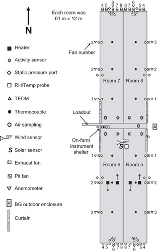
Figure 3. South-end view of barn 2, showing some of the measurement locations.

Each finishing room had two rows of 16 pens, which were 3.8 m × 5.8 m. The center walkway was 0.74 m wide. The concrete side wall was 0.93 m tall and 0.15 m thick. The finishing barns had fully-slatted concrete floors and manure was stored in a 2.4-m-deep pit under the floor. Reinforced concrete walls separated the pits of each room. However, there were 1.2 m × 0.15 m (L × H) liquid level equalization openings at the bottom of the center concrete walls to maintain the same manure levels between rooms. Manure was usually stored in the pit for about 6 months (about one rotation of finishing pigs) before removal.

Each room was independently and mechanically ventilated. There was 10 cm of cellulose insulation material in the attic. Outdoor air entered each room through a 12.0-m long, 1.3-m tall air inlet curtain that was located on the sidewalls (the east wall for the rooms located on the east side of the barn, and the west wall for rooms located on the west side of the barn) closest to the center hallway. The curtain opening was adjusted automatically according to the indoor temperature. Fresh air also entered the room from the attic through 24 ceiling diffusers, 0.6 m × 0.6 m, in two rows of 12 each along the length of the room.

There were five single-speed wall fans in the end walls of each room. The fans for the two north rooms and two south rooms were located in the north and south walls, respectively. There were also three evenly spaced and variable-speed, direct-drive fans of 0.61 m diameter (APP-24F, Automated Production Systems, Assumption, IL) along the outer sidewall of each room. These pit fans constituted the first two ventilation stages 1A and 1B as they operated together from low to high speeds. A direct-drive, single-speed, 0.91-m-diameter fan (APP-36X, Automated Production Systems), located in the center of the end wall, served as the second-stage fan. The other four, 1.22-m wall fans (APPB-50C, Automated Production Systems) operated in stages 3 through 5 (Table 1). Additional barn information is provided in Table 2.

Table 1. Fan numbers and ventilation stages for the finishing rooms

Stage	Quantity	Assigned fan number
1A	1	2 at variable speed 50% to 100%
1B	1 + 2 = 3	1, 2, 3 at 50% to 100% capacity
2	3 + 1 = 4	1, 2, 3, 6
3	4 + 1 = 5	1, 2, 3, 5, 6 *
4	5 + 1 = 6	1, 2, 3, 5, 6, 7 *
5	6 + 2 = 8	1, 2, 3, 4, 5, 6, 7, 8
*In room 5, staging for fans 5 and 7 was reversed; fan 7 was on stage 3, and fan 5 was on stage 4.

Table 2. Characteristics of the finishing barns

Descriptive parameters	Quad barn
Capacity, pigs	1000 per room × 4 rooms = 4000
Year of construction	2003
Barn orientation	North–south
Showering in/out requirement	None
Double stocking (i.e., 2000 pigs/room) during the first month of growth cycle	Rooms 5 and 6 only
Pig start weight, kg	5.6
Pig market (final) weight, kg	109–128
Roof slope	4:12
Sidewall height, m	2.4
Type of penning and floor	Steel bar, fully slatted floor
Type of feeders	Dry
Type of feed	Mash
Method of feed weighed	Feed mill scale
Water source	Groundwater well
Water consumption measurement	None
Drinker type and number	Two cup drinkers per pen
Duration of manure accumulation, d	78–196, average = 133
Frequency of power washing	Semiannually, between growth cycles
Disinfectant used in power wash	Yes
Heating	Gas-fired forced-air convection heater
Summer ventilation	Mechanical
Number of temperature sensors	2 per room
Emergency ventilation	Generator
Number of air inlets, ceiling diffuser	24 (2 rows of 12) per room
Dimensions of ceiling inlet	63.5 cm × 63.5 cm × 19.1 cm (L × W × H)
Inlet type	Ceiling
Inlet adjustment method	Automatic
Inlet control basis	Temperature
Controls vendor or manufacturer	Airstream

The farm was located on flat cropland with a 130 m × 130 m area of mature deciduous trees, located about 30 m north of the barns. The area between the barns and wooded area was mowed pasture area. Barn 1, located west of barn 2, represented the only other significant on-farm emission source. Besides an identical double-quad facility that was constructed and began operation in September 2008 about 300 m to the north of the current barns, there were no significant sources of NH₃ or H₂S within a 1.6-km radius around the farm site.

Emission monitoring was conducted in barn 2 according to the site monitoring plan shown in Figures 2 and 3. Because barn 2 was split into four rooms, with independent ventilation systems, each room was treated as an independent and separate “entity.” A storage area 5.0 m × 1.8 m in the southwest corner of the work area in barn 2 was converted to an on-farm instrument shelter (OFIS) for monitoring equipment and research personnel.

Operation, oversight and maintenance

A total of 152 and 132 visits were made during years 1 and 2, respectively. Remote access to the site computer via internet was used to ensure continuous data collection and to check for equipment malfunctions and abnormal readings. A total of 771 remote accesses were recorded in the log file. Data files and correspondence were emailed from the site computer on a daily basis.

Gas sampling and measurement

Gas sampling design and setup

In total, 17 gas-sampling locations (GSLs) were selected at the site. Exhaust air was sampled at the inlets of the 0.91-m fan (fan 6) and the three pit fans in each room (fans 1–3 in Figure 2). Thus, there were four gas-sampling locations in each room. Sampling probes at the 0.91-m fans were located approximately 0.5 m directly in front of the fan shutters, at the same height as the fan hub. The shutters were located inside of the barn, and closed automatically when fans were off for effective ventilation. The sampling probes for the pit fans were located underneath the concrete slat closest to the fan housing. Inlet air was sampled in front of the air inlet wall curtain of room 5 (Figure 2).

All gas-sampling locations were connected with Teflon tubing to a gas sampling system (GSS) (Heber et al., 2006), designed and constructed by Purdue University (West Lafayette, IN). One set of gas analyzers in the OFIS was sequenced through all 17 sampling locations, with 10-min sampling for each exhaust air location and 30-min sampling for barn inlet air. The gas analyzers included a photoacoustic infrared (PIR) CO₂ analyzer (model 3600, Mine Safety Appliances, Pittsburgh, PA), a fluorescence-based H₂S analyzer (model 450i, Thermo Fisher Scientific, Franklin, MA), and a photoacoustic multigas analyzer (PAMGA) (model 1412, Innova AirTech Instruments, Ballerup, Denmark), which was configured to measure NH₃, CH₄, ethanol, methanol, and total nonmethane hydrocarbons (determined by subtracting CH₄ from total hydrocarbons). For quality assurance and quality control purposes, methane and total nonmethane hydrocarbons were also measured with a nonmethane hydrocarbon analyzer (model 55C, Thermo Fisher Scientific).

Tests and maintenance of sampling system

The individual sampling lines were tested routinely for leaks. Fifty-liter Tedlar bags filled with single standard gas (usually NH₃) were also used for precision checks of all gas sampling lines. These tests were conducted to assess the performance of the entire gas sampling and measurement system with respect to precision and response (equilibration) time, and as a check for problems (leaks, pump failure, etc.). The quality assurance criteria for these checks were that the equilibrated concentrations must agree to within 10% of the known gas concentration.

Two types of GSS leak tests were conducted. The first test examined GSS integrity by briefly creating a “dead head” against the pump by closing all solenoid valves, while measuring exhaust airflow with a portable rotameter and recording the leakage flow with the GSS mass flow meter. The second test consisted of monitoring GSS flow and pressure after manually setting AirDAC (air data acquisition and control program) to sample from a particular GSL and plugging the sampling probe, which created a GSS manifold vacuum of about –70,000 Pa or 0.31 atm. The GSS flows under dead-head conditions that were 10% or less (<0.45 L/min) of the normal GSS flow rate of 4.5 L/min were indicative of leak-free operation under normal GSS manifold vacuums of –10,000 to –4,000 Pa (0.90–0.96 atm).

Concentration data validation

Time to equilibrium varied with different gases because of their inherent physical properties and influence, as well as length of sampling tubes. The first 7 min of the 10-min exhaust gas concentration data were discarded for NH₃ and NMHC, because the analyzer needed that much time (according to test results) to reach equilibrium after switching from one sampling location to another. The first 5 min of the 10-min exhaust gas concentration data were discarded for H₂S. Thus, the last 3 min of data of each sampling period were validated for NH₃ and NMHC, and the last 5 min of data of each sampling period were acceptable for H₂S. The time specified for gas concentration measurements to stabilize based on gas and sampling locations and the maximum interval for interpolating between two valid concentration measurements for a sampling location are given in Table 3.

Table 3. Gas concentration data validation and interpolation requirements

	Exhaust sampling locations		Inlet sampling location
Gas	Equilibration period, min	Maximum interpolation interval, min	Equilibration period, min	Maximum interpolation interval, min
NH3	7	300	10	3000
NMHC	7	300	10	3000
H2S	5	300	10	3000
CO2	3	300	5	3000
CH4	7	300	10	3000
CH3OH	7	300	10	3000
C2H5OH	7	300	10	3000

Gas analyzer precision checks and calibrations

Maintenance was scheduled for precision checks or calibrations of instrument and sensors. As an example, weekly zero/span or precision checks were conducted to monitor the gas sampling system and analyzer performance using gases with certified concentrations that were introduced via a challenge line at the room 6, fan 1 sampling location. Using this method, the calibration gases flowed through the same sampling system as actual barn air to reach the analyzers in the OFIS. Any precision check failure triggered further investigation for possible system leakage or analyzer sensitivity drifts and corrective action, which was followed by a new multipoint calibration and a precision check. The precision check data were plotted for long-term analyzer performance trends, quality assurance checks, and apparent failure of calibration gas integrity.

Tests of challenge line and filter cleanliness

To ensure operational performance and extend life spans of sensitive gas measurement instrumentation in dusty environments, it was important to protect gas analyzers from impurities in sample air using in-line membrane filters. However, these filters could potentially affect the overall response time, especially when enough PM was accumulated onto the filters to significantly absorb and desorb chemicals in the sample air stream. To study the effects of the challenge line and loaded filters, precision checks were conducted to deliver zero and span gases (NH₃, CH₄/THC [total hydrocarbon], C₂H₅OH, CH₃OH, H₂S, SO₂, and CO₂) as follows: (1) via the challenge line with a dirty filter, (2) via the challenge line with a new filter, and (3) directly into the Teflon gas sampling analyzer manifold. The sampling pump was disabled when the calibration gas was delivered directly to the analyzer manifold. The PM-laden filter had been accumulating PM for 1 month. The filter replacement was only conducted on an as-needed basis generally once every 4–8 weeks, and the replacement frequency varied with barn conditions. The 1-month period represented a case when there was appreciable PM accumulation onto the membrane filter. However, no attempt was made to determine the amount of PM collected on the filters. The filter sample was not collected and weighed. Based on the average PM₁₀ concentration (624.9 μg/m³) for that period, a constant sampling flow rate (3 L/min), and total sampling period, the estimated PM weight was 0.105 g. The total PM (with TSP) collected is expected to be more than 0.105 g.

Tests of sample integration time for the PAMGA analyzer

The operational principle of the PAMGA is based on the photoacoustic infrared detection method, and gas selectivity is achieved through the use of optical filters. With these filters, the PAMGA is able to measure the concentration of up to five gases plus water vapor in any air sample. Each individual optical filter is rotated in front of the photoacoustic chamber, and paused for a fixed sample integration time (SIT) before moving to the next filter. The default SIT was 5 sec for all optical filters. To reduce the response time, the SIT of individual filters can be modified to as low as 1 sec. To determine the best analyzer setting for this study, two SIT settings, the standard 5 sec and either 2 sec (NH₃, C₂H₅OH, and CH₃OH) or 1 sec (CH₄ and THC), were compared twice using certified calibration gases.

VOC sampling and measurement

Grab samples of VOC were collected near fan 6 and the TEOM sampling inlet in each room using 6-L stainless-steel canisters (TO-Can, Restek Corp, Bellefonte, PA) equipped with 0.64-cm (0.25-inch) bellows valves (Swagelok SS4H) and 207-kPa vacuum gauges. The sampling rate and period were 3.4 mL/min and 24 hr, respectively. Canister vacuum pressures were recorded at the beginning and end of the sampling periods for the calculation of total sample volumes. Sampling was conducted six times between June 1, 2009, and July 23, 2009, with duplicate samples typically collected at each location. Before sample collection, canisters were cleaned and passed quality control by testing 25% of the cleaned canisters. Canister samples were analyzed by Purdue University's Trace Contaminant Laboratory.

Particulate matter sampling and measurement

To obtain continuous barn inlet PM concentrations, an ambient PM monitor (Beta-Gage model FH62 C-14, Thermo Fisher Scientific) was installed 2 m away from the east wall of barn 2 (Figure 2) in an environmentally controlled enclosure. The sampling height of the inlet PM monitor was representative of the ambient air that flowed into the side curtains, which was a significant part of the inlet air in summertime. Operations such as tilling, planting, and harvesting in the crop field to the east likely contributed to inlet PM levels when they occurred during easterly winds. Northerly and southerly winds were likely to introduce some diluted exhaust air from the end wall fans in addition to crop related PM. Westerly winds may have created reentry of some pit fan exhaust air. A PM monitor with a tapered-element oscillating microbalance (TEOM model 1400a, Thermo Fisher Scientific) was used for the continuous measurement of exhaust PM concentrations, and was located 1 m upstream of the 0.91-m wall fan in each room (Figure 2), at the end of the center walkway. The PM₁₀ inlet heads on the TEOM and Beta-Gage were replaced with PM_2.5 heads for two 2-week periods beginning on January 10 and September 22, 2008, and February 4 (8 days) and July 1, 2009. The total suspended particulate (TSP) inlets were placed on the TEOMs and Beta-Gage eight times during the 2-year test, each time for 1 week or longer. To ensure quality data, the main flow and total flow rates were checked every 2 months, and mass transducer verifications were conducted at the same time. The TEOMs were also evaluated with collocated measurements of all three PM types. When conducting these side-by-side comparisons, two TEOMs were collocated near the inlet of fan 6 for several hours. The distance between the two collocated TEOM sampling inlets was 20 cm.

Ventilation system and barn control monitoring

Ventilation fan operation was monitored using a combination of three methods. First, auxiliary contacts of fan stage relays were monitored in 5-VDC circuits in conjunction with digital inputs of the data acquisition system, for stages 2 through 5. Second, fan speed sensors were mounted on each fan to monitor fan blade rotation. Third, open impeller anemometers (model 27106RS, R.M. Young Company, Traverse City, MI) were placed downstream of fan 6 of each room and pit fan 2 in room 7 (Figure 2).

Relays that controlled lights, soakers, misters, and feeders were monitored. Activity sensors (motion detector model SRN 2000, Visonic, Bloomfield, CT) were installed to monitor movement of animals and workers in the barns (Figures 2 and 3) and personnel in the OFIS.

Static pressure measurement

Static differential pressure (dP), necessary for calculating fan airflow rates, was measured across each barn wall that had fans (Figure 2). The measurement range of the static pressure sensors (model 260 MS3, Setra, Boxborough, MA) was –100 to +100 Pa, with an accuracy of ±1% of the full scale measurement. The sensors were routinely (total of 26 times) shunted for zero calibration checks, and to monitor for performance and drifts. Multipoint calibration checks were also conducted 12 times using a low-pressure calibrator (Micro-Cal 869, Setra, Boxborough, MA).

All dPs were corrected based on the results of zero-pressure checks. Calibration offsets were assigned to the different sensors based on time-weighted averages of the zero dP checks. The average dPs for each room were determined using validated data from both dP sensors in the room. In the event of a failed dP sensor, data of another functioning dP sensor in the same room was used.

Calibration of barn airflow rate

Accurate and repeatable fan airflow rate measurements are critical for aerial emission monitoring at mechanically ventilated barns. The airflow rates of the ventilation fans were determined in situ using a Fan Airflow Numeration System (FANS, U.S. Department of Agriculture [USDA]-invented portable airflow rate measurement system) (Gates et al., 2004) and a three-impeller-anemometer airflow monitoring system (TIAMS, a self-designed system for the variable-speed, 61-cm pit ventilation fans that the FANS could not access) (Lim et al., 2010). The simple wooden TIAMS was custom designed and constructed to fit the exhaust shrouds of the pit ventilation fans and to support three open impeller anemometers (model 27106R, R.M. Young, Traverse City, MI). The TIAMS was made of 1.3-cm-thick plywood and 5 cm × 5 cm lumber, with dimensions of 69 cm × 69 cm × 61 cm (W × H × D, where W and H are inside frame dimensions).

The TIAMS had three fixed heights of brackets to hold the anemometers, such that each single traverse measurement consisted of three sets of speed measurements at the three uniformly distributed heights. The heights and distances between the anemometers were distributed to facilitate uniform monitoring of the air speeds across the entire cross-sectional area. A Universal Serial Bus (USB)-based data-acquisition module (USB-1208FS, Measurement Computing, Norton, MA) was used to measure the anemometer voltage outputs. A custom program written in LabVIEW (National Instruments, Austin, TX) was used to receive and log the voltages. Analog signals of the anemometers were logged for 15 sec at each height. The measured airflow rate was calculated with the cross-sectional area of the TIAMS and the mean airflow speed. Both the FANS and the TIAMS were calibrated once at the Bioenvironmental and Structural Systems (BESS) Laboratory of the University of Illinois at Urbana–Champaign using an industry standard airflow measurement chamber. The group of FANS were upgraded and calibrated prior to commencing the monitoring.

Relative humidity and temperature measurement

Capacitance-type relative humidity and temperature probes (model RHT-WM, Novus Electronics, Porto Alegre, Brazil) were located at fan 6 in each room, and on a 1-m tower mounted on the roof of barn 2. Type T thermocouples were placed at each pit fan and near each heater (two per room) to monitor supplemental heating. One thermocouple was also placed in the OFIS near the gas analyzers. A pyranometer (LiCOR LI-200SL, Campbell Scientific, Logan, UT) and a wind anemometer and wind vane (model 03002VM Wind Sentry, R.M. Young Company, Traverse City, MI) were installed on the rooftop weather tower. The thermocouples were checked using an ice-water and warm-water bath together with precision liquid-in-glass thermometers (0.5°C precision).

Data acquisition and control

All data measured with on-line instruments and sensors were acquired by an on-site computer system (OSCS) (Ni et al., 2009; Ni and Heber, 2010), which consisted of a personal computer, custom software “AirDAC,” and data acquisition and control (DAC) hardware. The monitoring system at this site had 157 on-line measurement variables using different instruments and sensors. FieldPoint modules by National Instruments (Austin, TX) and USB devices by National Instrument (NI) and Measurement Computing (MC, Norton, MA) were selected for analog, digital, thermocouple, and counter inputs and digital output. Serial communication (RS232) was used to acquire data from the PAMGA multigas monitor and calibration variables (calibration time, gas concentration, etc.) from a gas diluter (model S-4040, Environics, Tolland, CT) for analyzer calibration. The OSCS also controlled sequential switching of multiple GSLs and the raceway heating system.

The AirDAC software averaged the acquired signals (after conversion to engineering units) over 15-sec and 60-sec intervals and recorded the means into two separate computer files. All real-time data were displayed in tabular and graphic forms for on-site or remote viewing using remote connection software (pcAnywhere version 12.0, Symantec, Mountain View, CA). Measurement alarms, data collection notifications, data files, graphs and statistics of the daily data sets, and modified configuration and field note files were automatically e-mailed to research personnel. This feature improved quality control of the monitoring and provided backup of data offsite within 24 hr after collection.

Manure sampling and analysis, and manure depth monitoring

Manure in the pit was sampled through the slatted floor 15 times from April 4, 2008 to August 21, 2009 (Table 2), to determine pH, solids content, and ammoniacal N. Manure was not agitated before sample collection. Beginning in November 2008, analyses of ash content of surface manure samples was introduced. During each sampling event, four pit surface samples were collected from locations along the center aisle, which was divided into four equal areas. The samples were collected from the top 0.31 m of the pit at the center point of each area using a 2.7-m long manure sampler (Coliwasa, Southeastern Liquid Analyzers, York, SC).

Additional core and surface samples were collected from the central sidewall pit access (fan 2) of each room, and tested for the same analytes as the inside surface samples. A total of eight core (load-out) samples (two per room) of manure were collected prior to pit emptying, and were analyzed for solids content, total N, and ash. Composite core samples were collected from two locations in each room. Each core sample consisted of four subsamples taken from either the north or south barn locations along the central aisle.

The manure depth was measured weekly beginning on September 7, 2007. The volume of manure pumped from the barns was measured by the producer using a dragline meter.

Feed and water sampling and animal inventory

On 10 occasions, a composite feed sample was collected from each side of the feeders in each room and analyzed for nitrogen and solids content by an independent laboratory (Midwest Laboratory, Omaha, NE). Equal subsamples from each of eight feeders were collected and mixed into a composite sample. Water was evaluated based on analyses of three samples of the site water supply, taken on November 10, 2008, and January 5 and February 16, 2009.

To facilitate a nitrogen mass balance, feed consumption rates were provided by the producer. The N content of the feed provided by the producer was checked against the feed samples collected in this study. The N content of the mortalities and the marketed pigs was determined from the literature (Gomez et al., 1999). The conceptual model incorporated N intake from feed, N retention in the pig body, and N loss into manure and air. Pig inventory information was recorded manually by the producer on a daily basis. The producer's inventory records were verified by counting the number of pigs and comparing the number with the corresponding number in on-farm inventory records and sales reports. The sales reports included the date, packing plant name, number of pigs transported, and total weight of each truckload. The average weight of incoming nursery pigs was supplied by the producer. The pigs of each room were grouped into subsets according to the date and average weight of each truckload. The weekly weight gain of each subgroup was estimated using the “standard” growth rate given in the Midwest Plan Service (MWPS) Swine Housing and Equipment Handbook (MWPS-8, 1983). For each subgroup, the weight gain in percentage of the final weight was calculated using the curve fitted to the beginning and final weights. The average pig weight was estimated based on daily gains of each subgroup, while the total inventory and total weight were the summation of each room's subgroups. Weekly mortality records were also taken into account in the calculation. The calculated average pig weight for the room was used to estimate the weight of mortalities.

Results and Discussion

Integrity of the gas sampling system and sampling lines

The results of the GSS leak tests, conducted on February 16, March 8 and 27, and July 18, 2009, demonstrated that the dead-head leakage flows were all less than the 0.45 L/min threshold. Because the system vacuum pressures were exceptionally high during the dead-head test conditions, the actual leakage during normal sampling conditions was negligible at this threshold. Systematic checking of individual sampling lines on September 14, 2007; February 19, March 8, April 25, and September 8, 2008; and January 7, March 27, and July 20, 2009, also confirmed the integrity of the sampling system. The results of the system response tests, discussed in the following sections, also demonstrated that the GSS and the sampling lines were leak-free (Figures 4 and 5), because the measured concentrations were similar.

Figure 4. Effects of the zero/span gas challenge line and loaded filter after one-month's exposure at average PM₁₀ concentration of 625 μg/m³, on the analyzer response time for (a) NH₃, (b) H₂S, (c) CH₄, and (d) CO₂.

Figure 5. Responses of CH₄ using 55C analyzer (calibration gas of 230 ppm, tested on November 14, 2008) and NH₃ using the PAMGA analyzer (calibration gas of 36 ppm, tested on January 9, 2009) at fan 6 sampling location of room 7.

It was observed that the in-line Teflon filter holders at the sampling locations and GSS inlets (two per sampling line) were the weak points that could easily cause leakage if they were not tightened correctly. However, if the leakage occurred at the sampling locations, or inlets of the sampling lines, it did not affect data quality because the leaking air would be the same as that of the sampling air. All other components within the GSS would be stressed during tests described earlier. The Teflon filters also provided a water barrier should water or manure accidently enter gas sampling inlets.

Effects of challenge line and filter cleanliness on response of gas measurement

The analyzers generally responded more quickly to the introduction of standard gas (36 ppm NH₃) when it was delivered directly to the analyzer manifold compared with delivering the standard gas to the challenge line (Figure 4). The concentration was chosen to be greater than the average to represent the worst case, so that leaks could be detected more easily. The instrument output approached an equilibrium concentration faster (less than 2.5 min) with the analyzer manifold method (Figure 4a). The challenge line method responded slower and with lower concentrations. The difference was probably caused by the length of additional plumbing and increased wetted surface area. With the challenge line, the standard gas was transported an additional 60 m (30 m one way) to the gas sampling manifold. The mean equilibrated (after 7-min equilibrium time) concentrations were 36.25, 36.65, and 37.18 ppm (three tests) using the challenge line with a PM-laden filter, the challenge line with a new filter, and the gas analyzer manifold, respectively. The linear range of the PAMGA for ammonia measurement was 0.2 ppm to 2000 ppm, while the stated precision was 1% of measured value, which equaled 0.36 ppm in this case. There was a slight difference (0.40 ppm) between the values observed for a PM-laden filter and a clean filter. However, a statistical test could not be conducted because of insufficient replications.

Ammonia adsorption by filters laden with swine PM led to about 30 sec longer response times than the new clean filter. Although the relationship between NH₃ adsorption and the amount of PM on the filters could not be quantified in this project, the tests confirmed findings in the literature that NH₃ adsorbs onto PM-loaded Teflon filters (Zhu et al., 2007). The differences between the three tests were generally similar to the magnitude of analyzer precision check drifts observed in weekly calibration checks over the 2-year study.

However, H₂S and SO₂ measurements responded faster when standard gases were delivered through the challenge line with a new filter than with the analyzer manifold method. This discrepancy may have been due to the sampling and data logging delays (60-sec averaging) of the 450i analyzer (Figure 4b), and the delayed responses of the gas diluter and gas sampling system. When the standard gas was introduced, research personnel did not attempt to identify and match the beginning of the 60-sec time integrated period; thus, the concentrations measured could be an artifact of calibration gas being introduced early in a cycle in one case, and near the end of a cycle in the other. Similar results were also observed for the SO₂ measurement. The responses to CH₄ measured by the PAMGA was the fastest (<1 min) when the span gas was delivered to the analyzer manifold (Figure 4c). In addition, measurements of CH₄ reached equilibrium in <2 min with all gas delivery methods and status of the filters. The NMHC concentrations measured by the PAMGA fluctuated between 1.0 and 1.5 ppm with a standard gas of 1.49 ppm concentration due to irreconcilable interferences by water vapor and other gases. However, the NMHC concentration measured with the 55C analyzer was more stable.

All three CO₂ tests indicated that the concentration reached steady state in <1 min. The response times were the shortest when the span gas was delivered to the analyzer manifold (Figure 4d). The results suggest that the effects of the challenge line delivery method, and the PM-laden filter were minimal for all gases except NH₃.

Effects of multi-gas analyzer's sample integration time

The test results showed very little difference between the two SIT settings for all gases (Table 4), especially when the analyzer was allowed to equilibrate for  >5 min. The standard deviations of the response concentrations were greater with an equilibrium time of 2 min compared with 5 min. The equilibrated mean concentrations were very similar for all the gases and both SITs. The results suggest that both SITs can be used for monitoring but the longer equilibrium time will obtain more stable measurements.

Table 4. Effects of the PAMGA's sample integration time (SIT) on gas measurements

		Concentration, ppm (SD)
				Equilibrium time
Gas	SIT, sec	Zero check difference (SD)	Standard gas	2 min	3 min
NH3	2	–0.40 (0.09)	35.9	37.0 (1.5)	37.8 (0.3)
	5	–0.11 (0.19)	35.9	35.0 (4.9)	37.2 (0.5)
CH4	1	0.30 (0.44)	229.3	233.7 (0.6)	233.8 (0.4)
	5	0.36 (0.42)	229.2	232.9 (0.5)	232.9 (0.5)
THC	1	–0.18 (0.03)	1.49	1.13 (0.08)	1.17 (0.04)
	5	–0.16 (0.02)	1.49	1.25 (0.04)	1.26 (0.03)
CH3OH	2	0.06 (0.11)	1.49	1.48 (0.10)	1.48 (0.09)
	5	0.00 (0.05)	1.50	1.47 (0.09)	1.49 (0.08)
C2H5OH	2	–0.03 (0.13)	1.99	1.50 (0.12)	1.52 (0.10)
	5	–0.04 (0.12)	1.99	1.48 (0.11)	1.52 (0.076)
Note: SD: Standard deviation.

Sampling line response time

The results of two response time tests using NH₃ (January 9, 2009) and CH₄ (November 14, 2008) confirmed leak-free conditions for the sampling line tested (Figure 5), because the measured concentrations matched the calibration gas concentrations. In addition, NH₃ required longer equilibrium times than CH₄. This proved that either calibration gas could be used to check the sampling system, provided there is sufficient equilibrium time.

TEOM performance

The results of the 27-hr collocation of the TEOMs in rooms 6 and 7 from July 6 to 7, 2009, showed very good agreement for PM₁₀ (Figure 6). The 29-hr collocation test of the TEOMs in rooms 5 and 8 from July 13, 2009, also showed similar results for PM₁₀ and TSP (room 5 vs. 8). The percentage difference between the mean concentrations was <5% for PM₁₀, <25% for TSP, but up to 154% for PM_2.5. The low agreement between the PM_2.5 measurements was probably caused by very low PM_2.5concentrations and insufficient equilibrium time. The minimum detection limit of TEOM was 0.06 µg/m³ (1-hr average). The reason for poor agreement in the rooms 6 and 7 TSP collocation remains unexplained. For the three collocation comparisons with good agreement, the slopes averaged 0.98 and the R ² values were above 0.96, indicating 1:1 relationships, especially for PM₁₀. The collocation test results were not applied to emission calculation as adjustment or correction factors.

Figure 6. Results of pairwise TEOM collocation for PM_2.5 (top), PM₁₀ (center) and TSP (bottom).

Thermocouple performance

The measurement responses of the thermocouple at fan 1 in room 5 after being immersed in ice-water and hot water baths are shown in Figure 7 as an example. The measurement readings approached calibration temperatures (0.5 and 61.0°C) in <2 min. The differences in temperature readings between the thermocouple and a standard mercury thermometer at ice-water and hot-water conditions were <0.2 and 0.5°C, respectively. All other thermocouples performed similarly and were within the quality control requirements of <2.0°C absolute difference. In principle and in practice, the thermocouple measurement is mature technology and yields linear measurement results. Therefore, no correction was needed for the thermocouple readings.

Figure 7. Response of thermocouple check using ice-water and hot-water baths at location fan 1 sampling location of room 5.

Responses of static pressure sensors to zero checks

The zero check records of the dP sensors indicated that most of the sensors were stable, with low standard deviations, and displayed similar overall drifts and trends. However, the dP sensors in room 6 showed an unusual drop in November and December 2008 (Figure 8). Although the reason for this is unexplained, the zero checks of this particular sensor later followed trends similar to those of the other sensors. A calibration offset was assigned to each sensor based on the time-weighted averages of its zero checks. Two sets of calibration factors were developed for the dP sensors based on 26 zero checks. Prior to December 6, 2008, the calibration offsets were 0.05 Pa (R5 East), –0.11 Pa (R5 South), 0.57 Pa (R6 South), –1.23 Pa (R6 West), –0.92 Pa (R7 North), 0.16 Pa (R7 West), 0.15 Pa (R8 East), and –0.05 Pa (R8 North). After December 6, 2008, the calibration offsets were –0.21 Pa (R5 East), –0.54 Pa (R5 South), –0.01 Pa (R6 South), –1.57 Pa (R6 West), –1.36 Pa (R7 North), –0.20 Pa (R7 West), 1.70 Pa (R8 East), and –0.36 Pa (R8 North). These results suggest that there were drifts in the sensor precision checks. However, the deviations of the sensors at zero output were <1% of the 200-Pa full measurement range.

Figure 8. Results of zero checks of dP sensors in rooms 5 and 6.

Application of FANS and TIAMS

Although the FANS could be applied to measure in situ ventilation fan performance with good repeatability, it could systematically underestimate fan capacity if the method was not properly calibrated, because the FANS itself restricted airflow and lowered ventilation fan performance. Therefore, the FANS should be calibrated while installed on the specific ventilation fan whenever possible.

The TIAMS provided 3 × 3 traverse measurements of the variable-speed pit ventilation fans. The TIAMS produced repetitive and linear measurements, which improved the overall assessment of the pit ventilation fan airflows.

The nominal performance of most commercial agricultural ventilation fans are typically available from the BESS Laboratory, which independently tests sample fans provided by manufacturers. Polynomial functions were fit through the BESS fan performance data. Fan performance degradation factors were determined based on the FANS and TIAMs field measurement data, and applied to all the polynomial functions. The procedures and equations are described in the literature (Chen et al., 2011).

Manure depth records

The manure depth records are shown in Figure 9. The lowest manure depth was 0.25 m after removal in the summer of 2009, while the highest manure accumulation was 1.45 m on August 8, 2008. The producer usually agitated and pumped out the manure from the pits in the spring and fall. However, additional pumping was also conducted in the summer of 2008.

Figure 9. Manure depths measured in the manure pit. Each arrow indicates manure load-out.

Recording pit manure depths is a convenient method for determining the quantity of manure in the facility. Together with the manure composition analysis, they provided valuable information for nitrogen mass-balance calculations, which can be used to estimate and predict NH₃ emission rates. Therefore, these data are critical and should be obtained frequently and consistently in comprehensive air quality studies on swine farms.

Barn inventory deviations

Comparison of two sets of barn inventory data, one set supplied by the producer and another set obtained by pig counting as a quality assurance measure on January 30, 2008, and February 6, 2009, showed acceptable deviations. The differences between the data sets from 2008 were 0, 5, 17, and 0 pigs per room, for rooms 5 to 8, respectively. The differences in the data sets from 2009 were 21, 21, 7, and 1 pigs per room for rooms 5 to 8, respectively. The largest difference of 21 pigs per room was 2.1% of the total number of pigs. These findings suggest that the inventory data supplied by the producer were reliable.

Conclusions

1.	Comprehensive and long-term air quality studies at commercial animal production facilities require complicated monitoring systems, large numbers of instruments and sensors, and detailed records of farm operations. System design, performance evaluation, routine maintenance, and quality assurance and quality control were essential to generate reliable measurement data.
2.	The integrity of the entire gas sampling system was critical for reliable gas concentration measurement. Different test methods (leak test, bag test, flow check, etc.) provided convenience for conducting quick GSS tests and complete system tests. Frequent sampling system checks, for example, weekly or daily, were necessary to ensure early problem detection and quality data collection.
3.	Calibration gases could be delivered to different locations of the sampling and measurement system. The effects of the challenge line delivery method and the effects of PM-laden filters on gas measurement response time were minimal for all gases except for NH3.
4.	Temperature measurements using thermocouples are accurate, reliable, and relatively inexpensive, and can be checked using an ice-water and warm-water bath together with precision liquid-in-glass thermometers (0.5°C precision). Differential static pressure measurements were necessary for accurate room ventilation calculations and were obtained with dP sensors.
5.	The equilibrium times of each of the measured gases depended on the gas, analyzer, and sampling tube length. With the same tubing length and same analyzer, NH3 required a longer equilibrium time than CH4, while both concentrations measured matched the calibration gas concentrations.
6.	Instrument variations of PM10 among different TEOM units were less than 5%. On the contrary, collocation comparisons conducted for PM2.5 and TSP concentrations showed differences up to 154% and 25%, respectively.
7.	While direct and continuous measurements of room ventilation rates were technically challenging, the use of the FANS and TIAMS significantly improved data quality by providing repetitive and accurate in situ fan performance measurements.
8.	Although the design and performance of the monitoring systems satisfied the objectives of the NAEMS, improvements can be made for future studies. Improvements include adding more automated calibration checks, acquiring data from instruments via serial communications (instead of analog inputs), and continuous manure depth measurement.

Acknowledgments

The financial support of the Agricultural Air Research Council and that of the National Pork Board are acknowledged.

References

- Aneja , V.P. , Arya , S.P. , Kim , D.S. , Rumsey , I.C. , Arkinson , H.L. , Semunegus , H. , Bajwa , K.S. , Dickey , D.A. , Stefanski , L.A. , Todd , L. , Mottus , K. , Robarge , W.P. and Williams , C.M. 2008 . Characterizing ammonia emissions from swine farms in eastern North Carolina: Part 1—Conventional lagoon and spray technology for waste treatment . Journal of Air Waste Management Association , 58 : 1130 – 1144 . doi: 10.3155-1047-3289.58.9.1130
- Battye , W. , Aneja , V.P. and Roelle , P.A. 2003 . Evaluation and improvement of ammonia emissions inventories . Atmospheric Environment , 37 : 3873 – 3883 . doi: 10.1016/S1352-2310(03)00343-1
- Chen , L. , Lim , T.-T. , Jin , Y. , Heber , A.J. , Ni , J.-Q. , Cortus , E.L. and Kilic , I. 2011 . Airflow rate calculation and uncertainty analysis for mechanically-ventilated swine finishing rooms , 19 – 22 . Chongqing , , China : Paper presented at the International Symposium on Health Environment and Animal Welfare . OctoberBeijing, China: Chinese Soceity of Agriculture Engineering.
- Gates , R.S. , Casey , K.D. , Xin , H. , Wheeler , E.E. and Simmons , J.D. 2004 . Fan assessment numeration system (FANS) design and calibration specifications . Transactions of ASAE , 47 ( 5 ) : 1709 – 1715 .
- Gomez , S. , Miller , P.S. , Lewis , A. and Chen , H.-Y. 1999 . Growth and carcass responses of barrows fed a corn-soybean meal diet or low-protein amino acid-supplemented diets at two feeding levels . Nebraska Swine Report , 131 : 35 – 39 .
- Heber , A.J. , Bogan , B.W. , Ni , J.-Q. , Lim , T.T. , Cortus , E.L. , Ramirez-Dorronsoro , J.C. , Diehl , C.A. , Hanni , S.M. , Xiao , C. , Casey , K.D. , Gooch , C.A. , Jacobson , L.D. , Koziel , J.A. , Mitloehner , F.M. , Ndegwa , P.M. , Robarge , W.P. , Wang , L. and Zhang , R. 2008 . The national air emissions monitoring study: Overview of barn sources. Paper presented at the Eighth International Livestock Environment Symposium (ILES VIII), Iguassu Falls, Brazil. St. Joseph, MI: ASABE Paper number PAP1459
- Heber , A.J. , Ni , J.-Q. , Lim , T.-T. , Schmidt , A.M. , Koziel , J.A. , Tao , P.C. , Beasley , D.B. , Hoff , S.J. , Nicolai , R.E. , Jacobson , L.D. and Zhang , Y. 2006 . Quality assured measurements of animal building emissions: Gas concentrations . Journal of Air Waste Management Association , 56 : 1472 – 1483 . doi: 10.1080/10473289.2006.10465680
- Lim , T.T. , Ni , J.-Q. , Heber , A.J. and Jin , Y. 13 September 2010 . “ Applications and calibrations of the FANS and traverse methods for barn air flow rate measurement ” . In International Symposium on Air Quality & Manure Management for Agriculture CD-Rom Proceedings , 13 September , MI : St. Joseph . ASABE
- 8 , MWPS- . 1983 . Swine Housing and Equipment Handbook , 4th , Ames , IA : Midwest Plan Service .
- National Research Council . 2003 . Air Emissions from Animal Feeding Operations: Current Knowledge, Future Needs , Washington , DC : National Academies Press .
- Ni , J.-Q. , Heber , A.J. , Darr , M.J. , Lim , T.T. , Diehl , C.A. and Bogan , B.W. 2009 . Air quality monitoring and on-site computer system for livestock and poultry environment studies . Transactions of ASABE , 52 : 937 – 947 .
- Ni , J.-Q. and Heber , A.J. 2010 . An on-site computer system for comprehensive agricultural air quality research . Computers and Electronics in Agriculture , 77 : 38 – 49 . doi: 10.1016/j.compag.2009.12.001
- Schiffman , S.S. , Graham , B.G. and Williams , C.M. 2008 . Dispersion modeling to compare alternative technologies for odor remediation at swine facilities . Journal of Air Waste Management Association , 58 : 1166 – 1176 . doi: 10.3155/1047-3289.58.9.1166
- Sun , G. , Guo , H. , Peterson , J. , Predicala , B. and Lague , C. 2008 . Diurnal odor, ammonia, hydrogen sulfide, and carbon dioxide emission profiles of confined swine grower/finisher rooms . Journal of Air Waste Management Association , 58 : 1434 – 1448 . doi: 10.3155-1047-3289.58.11.1434
- U.S. Environmental Protection Agency, Office of Air and Radiation. 2005. Health and environmental impacts of particulate matter http://www.epa.gov/oar/particlepollution/health.html (http://www.epa.gov/oar/particlepollution/health.html) (Accessed: 10 March 2009 ).
- Zhu , Z. , Xin , H. , Li , H. , Burns , R.T. and Dong , H. 2007 . Assessment of in-line dust filter type and condition on ammonia adsorption . Transactions of ASABE , 50 : 1823 – 1830 .